HAL Id: hal-00296819
https://hal.archives-ouvertes.fr/hal-00296819
Submitted on 22 Feb 2005
HAL is a multi-disciplinary open access
archive for the deposit and dissemination of
sci-entific research documents, whether they are
pub-lished or not. The documents may come from
teaching and research institutions in France or
abroad, or from public or private research centers.
L’archive ouverte pluridisciplinaire HAL, est
destinée au dépôt et à la diffusion de documents
scientifiques de niveau recherche, publiés ou non,
émanant des établissements d’enseignement et de
recherche français ou étrangers, des laboratoires
publics ou privés.
Tracking cyclones in regional model data: the future of
Mediterranean storms
M. Muskulus, D. Jacob
To cite this version:
M. Muskulus, D. Jacob. Tracking cyclones in regional model data: the future of Mediterranean storms.
Advances in Geosciences, European Geosciences Union, 2005, 2, pp.13-19. �hal-00296819�
SRef-ID: 1680-7359/adgeo/2005-2-13 European Geosciences Union
© 2005 Author(s). This work is licensed under a Creative Commons License.
Advances in
Geosciences
Tracking cyclones in regional model data: the future of
Mediterranean storms
M. Muskulus and D. Jacob
Max Planck Institute for Meteorology, Hamburg
Received: 24 October 2004 – Revised: 29 January 2005 – Accepted: 2 February 2005 – Published: 22 February 2005
Abstract. With the advent of regional climate modelling,
there are high–resolution data available for regional clima-tological change studies. Automatic tracking of cyclones in these datasets encounters problems with high spatial resolu-tion due to cyclone substructure. Watershed segmentaresolu-tion, a technique from image analysis, has been used to obtain estimates for the spatial extent of cyclones, enabling better tracking and precipitation analysis. In this study we have
used data from a 0.5◦Regional Model (REMO)
climatolog-ical model run for the period from 1961–2099, following the International Panel on Climate Change Special Report on Emissions Scenarios (IPCC SRES) B2 forcing. The re-sulting hourly mean sea level pressure (MSLP) fields have been analysed for cyclone numbers and tracks in the Mediter-ranean region. According to the results, the total number of cyclones in the Mediterranean seems to be increasing in the future, in spite of a general decrease of the numbers of stronger systems. In Summer, the increase in each gridbox seems to be proportional to the total number of cyclones in that box, whereas in Winter there is a slight proportional de-crease. As concerns track properties and precipitation esti-mates along tracks, no significant change could be detected.
1 Introduction
The Mediterranean is an area with high interest in cyclone climatology (for a qualification of this statement see the
pro-posal of the MEDEX project1). Objective cyclone tracking
methods have been first developed in this area by Alpert et al. (1990). More recently, there are the studies of Trigo et al. (1999), Picornell et al. (2001) and Maheras et al. (2001), as well as many others.
Correspondence to: M. Muskulus
1Jansa, A., Alpert, P., and Buzzi, A.: Cyclones that produce High Impact Weather in the Mediterranean, MEDEX, available from: http://medex.inm.uib.es/.
All of these studies concentrate on the analysis of past events, either from reanalysis data or operational weather models (Picornell et al., 2001). Most of the studies inves-tigate rather short periods. We have therefore used a regional climate model to investigate the Mediterranean climate on a large timescale of 139 years, particularly with respect to the mild B2 Global Warming scenario of the IPCC SRES (Naki-cenovic and Swart, 2000).
Cyclones have been detected by a local minimum search, and their time evolution has been tracked via a Kalman filter algorithm, both described below.
2 Data and Methodology
The data used in this study was derived from a REMO run for the period from 1961–2099. REMO is a three-dimensional hydrostatic atmospheric regional climate model which is scribed in Jacob (2001) and Jacob et al. (2001). It was de-veloped within the Baltic Sea Experiment (BALTEX) on the basis of the Europa Model of the German Weather Service
and runs in standard horizontal resolutions of 0.5◦, as well
as 1/6◦(not used in this study). The physical
parameteriza-tion for this run was provided by ECHAM4 physics, which is described in Roeckner et al. (1996).
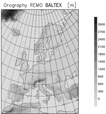
REMO version 5.1 introduced fractional areas of land, wa-ter and sea ice for each grid box, as well as monthly vary-ing vegetation characteristics. The standard domain size is 81×91 grid boxes and is shown in Fig. 1. The run under investigation was integrated from 1961–2099 with the IPCC SRES B2 scenario forcing. This scenario prescribes detailed amounts of anthropogenic emissions of greenhouse gases for each decade of the simulation, following a simulated story-line based on increased political concerns for environmen-tal issues and localized reactions (Nakicenovic and Swart, 2000). Of the four main IPCC SRES scenarios, this is one of the more optimistic ones.
14 M. Muskulus and D. Jacob: The future of Mediterranean storms
Fig. 1. The standard model domain: REMO BALTEX orography in
0.5◦resolution.
Fig. 2. The subregion used for the investigation of the Mediter-ranean.
The boundaries where provided by a T42 resolution run of the coupled Global Circulation Model ECHAM4/OPYC3, developed in cooperation between the Max Planck Institute for Meteorology, Hamburg, and the Deutsches Klimarechen-zentrum, Hamburg.
For the investigation of the Mediterranean, only a small part of the model domain was used, which is shown in Fig. 2. At each side, there are at least six grid boxes from the bor-ders of the larger domain to exclude undesired artifacts which could result from the (one–way) nesting of the REMO do-main in the global ECHAM4/OPYC3 grid.
The analysis has been performed on the hourly mean sea
level pressure output field. Due to the high resolution (0.5◦
and 1 hr for horizontal and time resolutions, respectively) no further data (wind speed, vorticity, etc.) were considered.
2.1 The Watershed Segmentation Method
The method proceeds by finding local minima of MSLP, hereafter referred to as events, in the Von–Neumann neigh-bourhood consisting of the eight nearest grid boxes. Events with more than 1015 hPa MSLP will not be considered. For each event certain characteristics are estimated, including the Laplacian (via a linear filter) as a measure of strength, fol-lowing Murray and Simmonds (1991), and the so called wa-tershed extent and wawa-tershed area as objective measures of the area under the cyclone’s influence.
From the gridded MSLP field, the watersheds will be found by a modified version of the fast watershed algorithm described in Vincent and Soille (1991): Starting from the gridded MSLP field, all pixels will be removed from the grid and sorted according to their MSLP value. Step by step, sim-ulating a flooding of the MSLP landscape, the pixels will be put on the grid back again in the sorted order. If a pixel is isolated on the grid after placing, it will start a new region. Otherwise, if a pixel is adjacent to one or more pixels of one already existent region, it will become part of that region too. If it is adjacent to two or more different regions, it will be-come a watershed border. In fact, as we are also interested in anticyclones, at each step our algorithm places the low-est as well as the highlow-est still remaining pixels on the grid. An example of the application can be seen in Fig. 4, where the result of the watershed segmentation of the pressure field from Fig. 3 is shown.
The usefulness of the watershed segmentation lies in its easy, robust and fast implementation and its objectiveness in giving a spatial estimate of cyclonic influence. As we are interested in analysing the precipitation connected with moving cyclones and considering that the precipitating front will not be at the position of the local pressure minimum, but somewhere nearby, this fact is essential for our purposes. For each event, the area of its watershed region is considered, as well as the radius of the largest circle around the minimum which still fits into it, which will be called watershed extent. To facilitate analysis of precipitation, for each event we consider the (spatial) maximum of precipitation (per grid box) in its extent circle and the (spatial) precipitation sum in its extent circle, as well as in its watershed region. This gives a rough estimate of the precipitation connected with the cyclone on a hourly basis, as a starting point for further studies.
2.2 Cyclone tracking
The tracking is done via a Kalman filtering approach (Black-man (1986), Brookner (1998)), which has certain advantages over the traditional backtracking. In the usual approach, the gridded fields at only two consecutive timesteps are consid-ered. Using a Kalman filter, it is possible to include informa-tion about the whole cyclonic history. Another advantage is the error estimate from the filter (times two in our analysis), which directly translates to a gating bound, i.e. a maximum distance in which to search for the next corresponding event,
Fig. 3. Example MSLP field for the application of the watershed (WSH) segmentation algorithm.
Fig. 4. The result of the application of the watershed segmentation
algorithm. Watershed borders have been drawn in black in an ex-aggerated way. Circles in white show the location of local minima and maxima. The lighter shade corresponds to minima, whereas the darker shade corresponds to maxima of the pressure field.
for the matching algorithm. The model underlying the filter was chosen to be a linear constant velocity model, both for its simplicity, as well as for its performance. In the future, this could be replaced by a more realistic model. The matching is done by minimizing a weighted prediction error function that takes into account distance, intensity, value and extent of
Fig. 5. Monthly numbers of cyclone exposure hours in Winter for
the whole period. (Smoothed, see text).
Fig. 6. Monthly numbers of cyclone exposure hours in Summer for the whole period. (Smoothed, see text).
the events. The weights have been derived empirically from the variance of the data.
We only consider tracks which exist for at least 12 h and which show a minimal central pressure of 1000 hPa or below once during their lifetime.
3 Results
3.1 Cyclogenesis over the Mediterranean
Fig. 5 shows the mean monthly numbers of cyclones in Win-ter. These are calculated as follows: For each grid box of the study domain we counted the number of cyclone cen-ters falling into the box per timestep. These numbers have been summed up over the whole simulation period, and the resulting distribution has been divided by the number of years times months in the season. We will call this quantity monthly exposure hours in the following. For better visual-ization, a 2d Gaussian filter with a radius of four grid boxes has been applied to smooth the data in this and the following figures.
One can clearly see the Genoa center with counts as high as 15 monthly exposure hours in one grid box (not dis-cernible on the figure), as well as some activity in the Aegean
16 M. Muskulus and D. Jacob: The future of Mediterranean storms
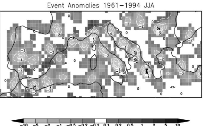
Fig. 7. Monthly anomalies in cyclone exposure hours for the period
from 1961–1994 in Summer. (Smoothed, see text).
Fig. 8. Monthly anomalies in cyclone exposure hours for the period
from 1995–2029 in Summer. (Smoothed, see text).
Sea and along the Adriatic coast. This result seems to be in good agreement with recent studies (see for example Ma-heras et al., 2001). Interestingly, it is important to point out the presence of a second center just off the coast in North Eastern Italy with counts as high as 11 monthly exposure hours in one box, which has not been found in previous stud-ies. This discrepancy could be an effect of the day–night cycle, with orography induced thermal lows playing a major role, due to the use of hourly data instead of the six hourly or twelve hourly data used by other authors. The phenomenon itself seems to be known to the Italian Weather Service in the area, and is partially attributed to a similar (lee-) cyclogene-sis mechanism (due to the Eastern Alps) as in the Genoa case (private communication).
In Summer (Fig. 6), there is strong activity in the Genoa center with counts as high as 53 exposure hours in one box, and even counts of 74 in the nearby North-Eastern Italy area. There is also activity visible along the Spanish coast and in Central Spain. Some remnants of the Saharan and the Cyprus cyclones can be seen at the borders of the study region. The unexpected activity over the Aegean sea could be explained as the effect of a day-night cycle, as in the case of the cy-clones over North-Eastern Italy.
Fig. 9. Monthly anomalies in cyclone exposure hours for the period
from 2030–2064 in Summer. (Smoothed, see text).
Fig. 10. Monthly anomalies in cyclone exposure hours for the
pe-riod from 2065–2099 in Summer. (Smoothed, see text).
The other two seasons (not shown) are characterized by intermediate numbers between the extremes of Summer and Winter. In the following we will therefore concentrate on those two seasons only.
The period of analysis has been divided into four different time intervals; each time interval is 35 years long, with the exception of the first which is only 34 years. On Figs. 7, 8, 9 and 10 the anomalies of summer cyclone activity through-out the whole period of simulation are plotted: As before, the output has been smoothed by a 2d Gaussian filter with a radius of four grid boxes. Particularly, Fig. 7 displays pre-dominant negative anomalies, that means a number of cy-clones below the mean value of the study period. Going through Fig. 8 for the period 1995–2029 and Fig. 9 for the years 2030–2064 until Fig. 10 for the years 2065–2099 one sees a steady increase in the number of cyclones, which is almost proportional to the mean number from Fig. 6. This climatological effect can not be seen in Winter, where there is even a slight decrease of numbers in the Genoa region (not shown). As one believes that during Global Warming sce-narios the sub–tropical belt should extend northwardly (H. G¨ottel, private communication), one would expect a decrease in cyclone numbers in summer as in winter, but according to the results of our experiments it seems to be not the case.
Table 1. Total cyclone exposure hours in four different periods for
the Mediterranean area.
Period <1015 hPa <995 hPa 1961–1994 899 853 12 952 1995–2029 1 040 175 10 294 2030–2064 1 156 301 11 235 2065–2099 1 276 086 9688
Table 2. The same as in Tab. 1, but only for Summer.
Period JJA <1015 hPa JJA <995 hPa
1961–1994 450 993 60
1995–2029 557 954 166
2030–2064 648 671 19
2065–2099 723 168 78
In fact the first column of Table 1 shows an increase in cy-clone events for the whole period of simulation; this result is confirmed taking into account only the Summer cyclones (Table 2, first column). But if we consider only strong sys-tems below 995 hPa (which seldom occur in Summer), we can see a meaningful decrease in cyclone numbers (Table 1, second column), whereas in Summer the numbers are some-what unconclusive (Table 2, second column).
3.2 Cyclone tracks and dynamics
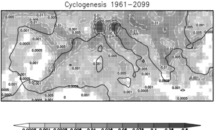
To get a better picture, we also analyse cyclone tracks. In Fig. 11 one sees the mean monthly cyclogenesis numbers, where the Gulf of Genoa dominates, as well as the North Ital-ian centre. These are calculated similar to the monthly expo-sure hours by counting all first occurences of cyclone centers from a track in their grid box over the whole study period and then dividing by the total number of months. Comparing this with the cyclolysis numbers from Fig. 12 one sees that these regions are also involved in dissolving cyclones, a fur-ther indication that fur-there might be many stationary, shallow cyclones involved, although the budget (cyclogenesis minus cyclolysis) for these regions is positive, meaning that there are a lot of moving systems as well. Many of them leave the area in a north, north–easterly direction, on which the cyclol-ysis plot gives some indication.
Track lengths in hours, i.e. the number of hours between detection and loss of track, are shown in Fig. 13. In interpret-ing this figure one should remember that only tracks with a minimum lifetime of 12 h have been considered. One can recognize many long–living systems, and comparing with Fig. 14, where the linear length between cyclogenesis and cy-clolysis is depicted, one can see that these systems are mov-ing on average more than 10 grid boxes, which is more than 500 km.
The maximum deepening rate in Fig. 15 is estimated by the maximum of the differences in MSLP from one timestep
Fig. 11. Mean monthly cyclogenesis numbers. (Smoothed, see text).
Fig. 12. Mean monthly cyclolysis numbers. (Smoothed, see text).
to the next. The hourly rates thus found have been multiplied by six for comparison with the usual rates derived from six hourly data (see for example Trigo et al., 1999). This leads to seemingly much higher rates than in the case of those rates implicitly smoothed by their lower sampling rate. Our rates have also not been corrected geostrophically. Still the fig-ure contains useful information: A considerable tail of fast– deepening systems can be seen (the highest values will prob-ably be due to tracking errors which can result in jumps of the central MSLP value from one timestep to the next) and it indicates that deepening of cyclones might take place with considerable variability in the deepening rate, leading to the observed high values of the maximum rate.
In Fig. 16 the maximum watershed extent along the track is depicted. The shape of the distribution closely resembles the result for the cyclone radius from Trigo et al. (1999). The maximum at six grid boxes corresponds to a realistic cyclone extent of about 300 km.
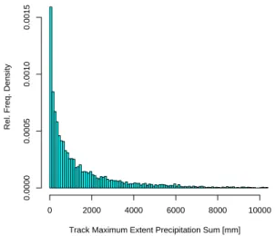
Concerning precipitation, in Fig. 17 the precipitation sum on the watershed extent area along the track is shown. This is an indicator of the total precipitation brought about by the cyclone; it is calculated by summing up all precipita-tion amounts in the extent circle for all timesteps that the cyclone track exists. In the future, this relatively coarse mea-sure could be replaced by a finer analysis taking into account
18 M. Muskulus and D. Jacob: The future of Mediterranean storms 0 50 100 150 200 0.00 0.01 0.02 0.03 0.04 Track Lifetime [hr]
Rel. Freq. Density
Fig. 13. Cyclone lifetime histogram.
0 10 20 30 40 50 60 70 0.00 0.01 0.02 0.03 0.04 0.05 0.06
Linear Track Length [boxes]
Rel. Freq. Density
Fig. 14. Cyclone track length histogram. The numbers shown are
linear distances between cyclogenesis and cyclolysis points in grid boxes (which are spaced on average 51 km apart).
differences in temporal and spatial precipitation patterns. On this coarse level though, we see that most of the systems are precipitating. There is also a substantial tail of heavily pre-cipitating tracks discernible. It is of high interest to under-stand which cyclone tracks correspond to these high precipi-tation events and why.
4 Conclusions
The run under analysis with its 139 years has been used to study cyclone behaviour in the Mediterranean, from a clima-tological viewpoint as well as from a climate change point of view. The data shows familiar features (e.g. the Genoa cyclone center, the shape of the cyclone extent distribution) from other studies. Furthermore, a second center in North-Eastern Italy has been found, which in previous studies with temporal resolutions of six hours or more has not been seen. Concerning possible climatic change due to the enforced
0 5 10 15 20 25 30 35 0.00 0.02 0.04 0.06 0.08 0.10 0.12 0.14
Track Maximum Deepening Rate [hPa/6hr]
Rel. Freq. Density
Fig. 15. Cyclone maximum deepening rates in hPa per six hours
(estimated from hourly differences, see text).
0 5 10 15 20 25 30 0.00 0.05 0.10 0.15 0.20
Track Maximum Extent [boxes]
Rel. Freq. Density
Fig. 16. Cyclone maximum extent in grid boxes.
Global Warming scenario, there seems to be an increase in shallow, possibly thermal, cyclones in all seasons, pointing to an intensification of the generating mechanisms. Interest-ingly, strong systems in Winter seem to decrease, pointing to a possible northward shift in major cyclone tracks that could be studied with more detail in a future work. There is no sig-nificant change in precipitation patterns or track statistics to be stated for tracks longer than 12 h in the four periods under investigation at this level of the analysis, which is somewhat surprising.
It would be desirable to enhance the analysis of these data in the future by addressing specific mechanisms of cyclone
generation and movement. Especially cyclones that pass
through the Genoa region are of considerable interest for Mediterranean as well as Central European climate. In re-cent years, major flooding events in Europe have been caused by Genoa cyclones following the so-called Vb track (van Bebber, 1891, see also Bahrenberg, 1973.). Therefore, an
0 2000 4000 6000 8000 10000
0.0000
0.0005
0.0010
0.0015
Track Maximum Extent Precipitation Sum [mm]
Rel. Freq. Density
Fig. 17. Total cyclone precipitation in the extent circle, summed
over the whole track.
analysis of these tracks with our methods, especially with re-gard to precipitation would be highly desirable.
For the precipitation analysis, finer measures are needed which take into account the differences in spatial and tempo-ral characteristics of precipitating cyclones. A classification via clustering methods would also be interesting.
The question of how to classify high precipitation (Genoa) cyclones from these data and the nontrivial question of how to quantify their impact on European climate will therefore be addressed in a future work.
Acknowledgements. We are grateful for technical assistance by R. Podzun. We also wish to thank two anonymous reviewers for their valuable comments.
Edited by: L. Ferraris
Reviewed by: anonymous referees
References
Alpert, P., Neeman, B., and Shay-El, Y.: Climatological analysis of Mediterranean cyclones using ECMWF data, Tellus A, 42, 65– 77, 1990.
Bahrenberg, G.: Auftreten und Zugrichtung von Tiefdruckgebi-eten in Mitteleuropa, Ph.D. Thesis, Institut f¨ur Geographie und L¨anderkunde, Universit¨at M¨unster, 1973.
Blackman, S. S.: Multiple–Target Tracking with Radar Applica-tions, Artech House, Inc., 1986.
Brookner, E.: Tracking and Kalman filtering made easy, Wiley-Interscience, 1998.
Jacob, D.: A note to the simulation of the annual and inter-annual variability of the water budget over the Baltic Sea drainage basin, Meteor. Atm., 77, 61–73, 2001.
Jacob, D., Andrae, U., Elgered, G., et al.: A Comprehensive Model Intercomparison Study Investigating the Water Budget during the BALTEX–PIDCAP Period, Meteor. Atm., 77, 19–43, 2001. Maheras, P., Flocas, H., Patrikas, I., and Anagnostopoulou, C.: A 40
Year Objective Climatology of Surface Cyclones in the Mediter-ranean Region: Spatial and Temporal Distribution, Int. J. Clim., 21, 109–130, 2001.
Murray, R. and Simmonds, I.: A numerical scheme for tracking cy-clone centres from digital data. Part I: development and operation of the scheme, Aust. Meteor., 39, 155–166, 1991.
Nakicenovic, N. and Swart, R. (Eds): Emissions Scenarios. A Spe-cial Report of Working Group III of the Intergovernmental Panel on Climate Change, Cambridge University Press, 2000. Picornell, M., Jansa, A., Genoves, A., and Campins, J.: Automated
Database of Mesocyclones from the HIRLAM(INM)-0.5◦ Anal-yses in the Western Mediterranean, Int. J. Clim., 21, 335–354, 2001.
Roeckner, E., Arpe, K., Bengtsson, L., et al.: The atmospheric gen-eral circulation model ECHAM4: Model description and simula-tion of present-day climate, Tech. Rep. 218, Max Planck Institute for Meteorology, Hamburg, 1996.
Trigo, I., Davies, T., and Bigg, G.: Objective Climatology of Cy-clones in the Mediterranean Region, J. Climate, 12, 1685–1696, 1999.
van Bebber, W.: Die Zugstrassen der barometrischen Minima, Met. Z., 8, 361–366, 1891.
Vincent, L. and Soille, P.: Watersheds in digital spaces: an efficient algorithm based on immersion solutions, IEEE Patt. A., 13, 583– 598, 1991.