Trends in the ionospheric E and F regions over Europe

HAL Id: hal-00316431

https://hal.archives-ouvertes.fr/hal-00316431

Submitted on 1 Jan 1998

HAL is a multi-disciplinary open access

archive for the deposit and dissemination of sci-entific research documents, whether they are pub-lished or not. The documents may come from teaching and research institutions in France or abroad, or from public or private research centers.

L’archive ouverte pluridisciplinaire HAL, est destinée au dépôt et à la diffusion de documents scientifiques de niveau recherche, publiés ou non, émanant des établissements d’enseignement et de recherche français ou étrangers, des laboratoires publics ou privés.

J. Bremer

To cite this version:

J. Bremer. Trends in the ionospheric E and F regions over Europe. Annales Geophysicae, European Geosciences Union, 1998, 16 (8), pp.986-996. �hal-00316431�

Trends in the ionospheric E and F regions over Europe

J. Bremer

Institut fuÈr AtmosphaÈrenphysik, Schloûstr. 6, D-18225 KuÈhlungsborn, Germany Received: 12 November 1997 / Revised: 9 March 1998 / Accepted: 11 March 1998

Abstract. Continuous observations in the ionospheric E and F regions have been regularly carried out since the ®fties of this century at many ionosonde stations. Using these data from 31 European stations long-term trends have been derived for di€erent parameters of the ionospheric E layer (h¢ E, foE), F1 layer (foF1) and F2 layer (hmF2, foF2). The detected trends in the E and F1 layers (lowering of the E region height h¢E; increase of the peak electron densities of the E and F1 layers, foE and foF1) are in qualitative agreement with model predictions of an increasing atmospheric greenhouse e€ect. In the F2 region, however, the results are more complex. Whereas in the European region west of 30° E negative trends in hmF2 (peak height of the F2 layer) and in the peak electron density (foF2) have been found, in the eastern part of Europe (east of 30° E) positive trends dominate in both parameters. These marked longitudinal di€erences cannot be explained by an increasing greenhouse e€ect only, here probably dy-namical e€ects in the F2 layer seem to play an essential role.

Key words Atmospheric composition and structure (Pressure, density and temperature) á Ionosphere (Mid-latitude ionosphere) á Radio science (Ionospheric propagation).

1 Introduction

Based on the results by Roble and Dickinson (1989) with a globally averaged model of the coupled meso-, thermo- and ionosphere, Rishbeth (1990) predicted a lowering of E and F2 peak heights (hmE, hmF2) by about 2.5 km and 15±20 km if the atmospheric CO2and CH4content is doubled. The expected changes in the E and F2 peak electron densities should be small. In a more recent paper Rishbeth and Roble (1992)

investi-gated the atmospheric greenhouse e€ect for December solstice conditions with the 3-dimensional TIGCM (thermosphere/ionosphere general circulation model) developed at the National Center for Atmospheric Research, Boulder. Assuming again a doubling of the greenhouse gases, a lowering of hmF2 by 10±20 km was derived whereas the electron density at the peak height of the F2 layer and above decreases (foF2 decreases up to 0.5 MHz) but below the F2 peak the electron density increases (including F1 and E regions).

Using the data of individual ionosonde stations Bremer (1992) with observations from Juliusruh and Poitiers and more recently Ulich and Turunen (1997a) with data from SodankylaÈ found a signi®cant lowering in hmF2 during the last 40 years. Recent investigations by Bremer (1996, 1997a,b) and by Ulich and Turunen (1997b) gave, however, some hints that the trends in the F2 region are not so uniform as expected. Therefore, in this study the data of all available European ionosonde stations are considered to provide more reliable results about the thermospheric trends in dependence on latitude, longitude and altitude. In these analyses characteristic parameters of the F2 layer (hmF2, foF2), of the F1 layer (foF1) and of the E layer (h¢E, foE) have been used. The large amount of data necessary for these investigations were extracted from di€erent CD-ROMs of the National Geophysical Data Center (NGDC), Boulder, Colorado, USA and from the WDC-C at the Rutherford Appleton Laboratory (RAL), Chilton, Did-cot, UK.

2 Experimental data and data analysis

Data from 31 European ionosonde stations (5° W ± 70° E, 35° N ±70° N) have been used for trend analyses. In Table 1 these stations are presented in dependence on latitude. The trend coecients given will be discussed later in Sects. 3 and 4.

In the trend analyses we used only monthly median values of the di€erent ionosonde parameters. It is well-known that these parameters depend markedly on solar

and geomagnetic activity. To detect relatively small trends in the ionospheric parameters it is therefore necessary to remove these strong in¯uences, e. g. by a simple regression analysis. We calculated for the exper-imental data X (X ˆ hmF2, foF2, foF1,h¢E or foE) for each complete hour (0±23 UT) and each month the following regression equations

Xthˆ A ‡ B R ‡ C Ap: …1†

Here R is the solar sunspot number and Ap the planetary geomagnetic activity index. Instead of R also the solar ¯ux data F 10.7 can be used to characterize the solar activity, the results of the trend analysis do not depend on this choice. Using the results of the regression analysis after Eq. (1) we calculated the deviations DX of the experimental hourly data X exp from these theoret-ical values Xth

DX ˆ Xexpÿ Xth: …2†

With these DX values linear trends can be estimated according to

DX ˆ a ‡ b year: …3†

In this way it is possible to derive trend parameters b for each hour and each month. In this work the hourly and monthly DX values have normally been averaged to

calculate more reliable yearly DX values and yearly trends after Eq (3).

The test of the signi®cance of the trend parameter b can be made with Fisher's F parameter

F ˆ r2_{N ÿ 2†=…1 ÿ r}2_{†: …4†}

Here r is the correlation coecient between DX and year after Eq. (3), and N is the number of years used in the analysis. The signi®cance levels to be exceeded by the F parameter after Eq. (4) can be found in Taubenheim (1969). Signi®cant trends with a con®dence level of more than 90% are maked in Table 1 or with solid symbols in Figs. 1±6.

3 Results 3.1 F2 region

The peak height of the F2 layer (hmF2) and the electron density at this height (foF2) are used in the trend investigations of the F2 region. The value of hmF2 was derived from observed monthly M(3000)F2 values using the well-known formula of Shimazaki (1955)

hmF2 ˆ 1490=M…3000†F2 ÿ 176: …5†

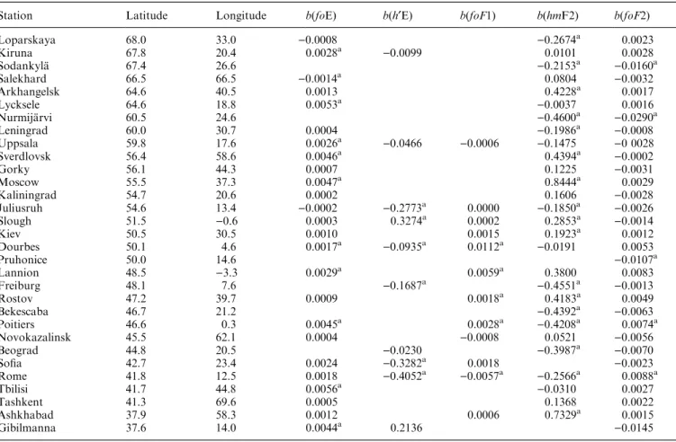
Table 1. Ionosonde stations with geographic coordinates (latitude and longitude) and trend coe€cients b derived for di€erent characteristic parameters of the ionospheric E, F1 and F2 regions

Station Latitude Longitude b(foE) b(h¢E) b(foF1) b(hmF2) b(foF2)

Loparskaya 68.0 33.0 )0.0008 )0.2674a _0.0023 Kiruna 67.8 20.4 0.0028a _{)0.0099 0.0101 0.0028} SodankylaÈ 67.4 26.6 )0.2153a _)0.0160a Salekhard 66.5 66.5 )0.0014a _{0.0804 )0.0032} Arkhangelsk 64.6 40.5 0.0013 0.4228a _0.0017 Lycksele 64.6 18.8 0.0053a _{)0.0037 0.0016} NurmijaÈrvi 60.5 24.6 )0.4600a _)0.0290a Leningrad 60.0 30.7 0.0004 )0.1986a _)0.0008 Uppsala 59.8 17.6 0.0026a _{)0.0466 )0.0006 )0.1475 )0 0028} Sverdlovsk 56.4 58.6 0.0046a _0.4394a _)0.0002 Gorky 56.1 44.3 0.0007 0.1225 )0.0031 Moscow 55.5 37.3 0.0047a _0.8444a _0.0029 Kaliningrad 54.7 20.6 0.0002 0.1606 )0.0028 Juliusruh 54.6 13.4 )0.0002 )0.2773a _{0.0000 )0.1850}a _)0.0026 Slough 51.5 )0.6 0.0003 0.3274a _{0.0002 0.2853}a _)0.0014 Kiev 50.5 30.5 0.0010 0.0015 0.1923a _0.0012 Dourbes 50.1 4.6 0.0017a _)0.0935a _0.0112a _{)0.0191 0.0053} Pruhonice 50.0 14.6 )0.0107a Lannion 48.5 )3.3 0.0029a _0.0059a _{0.3800 0.0083} Freiburg 48.1 7.6 )0.1687a _)0.4551a _)0.0013 Rostov 47.2 39.7 0.0009 0.0018a _0.4183a _0.0049 Bekescaba 46.7 21.2 )0.4392a _)0.0063 Poitiers 46.6 0.3 0.0045a _0.0028a _)0.4208a _0.0074a Novokazalinsk 45.5 62.1 0.0004 )0.0008 0.0521 )0.0056 Beograd 44.8 20.5 )0.0230 )0.3987a _)0.0070 So®a 42.7 23.4 0.0024 )0.3282a _{0.0018 )0.0023} Rome 41.8 12.5 0.0018 )0.4052a _)0.0057a _)0.2566a _0.0088a Tbilisi 41.7 44.8 0.0056a _{)0.0310 0.0027} Tashkent 41.3 69.6 0.0005 0.1368 0.0022 Ashkhabad 37.9 58.3 0.0012 0.0006 0.7329a _0.0015 Gibilmanna 37.6 14.0 0.0044a _{0.2136 )0.0145}

As shown by Bremer (1992) the choice of this simple formula is not critical for the derived trends, the trends are nearly identical if the more accurate for-mula of Bilitza et al. (1979) is used for the estimation of hmF2.

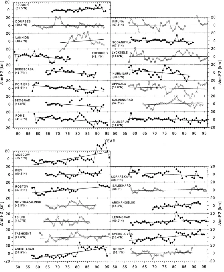
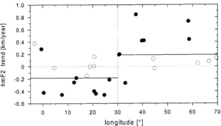
In Fig. 1 the results of the trend analysis for hmF2 values are separately presented for European stations at longitudes less than 30° E in the upper part of this ®gure and at longitudes greater than 30° E in the lower part. In both cases the trends are ordered in dependence on latitude, shown in brackets below the name of the station. If the linear trends are signi®cant with more than 90% the yearly data DhmF2 are presented by solid dots, if the signi®cance level is smaller than 90% open circles have been used. The numerical values of the derived trend coecients can be found in Table 1. Whereas the trends do not show a dependence on latitude in the latitudinal belt investigated between 35° N and 70° N, there are marked di€erences between the two longitudinal regions west and east of 30° E. In the part west of 30° E 11 of 15 trends are negative, from 9 signi®cant trends are even 8 negative. In the eastern part of Europe (east of 30° E) the results are quite opposite. Eleven of 13 trends including 7 of 8 signi®cant trends are positive. This marked di€erence can also be seen in Fig. 2 where the hmF2 trend parameters are shown in relation to longitude. The two straight lines mark the median values of the individual trends in the two longitudinal zones: )0.18 km/y and 0.19 km\y. The corresponding mean values for both regions which slightly deviate from the median values shown in Fig. 2 are signi®cantly di€erent with more than 99% as can easily be shown by a t-test (Tau-benheim 1969).

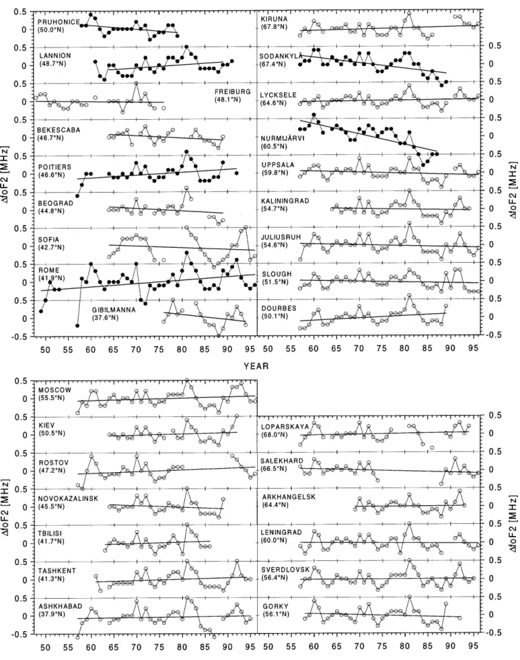
The trends of foF2 are presented in Fig. 3 in a similar way as for hmF2 in Fig. 1. Also the foF2 trends do not markedly depend on latitude. But there seems to exist again a di€erence between the two longitudinal regions west or east of 30° E. The median values of the foF2 trends are: )0.0024 MHz/y for the western part (stations in the upper part of Fig. 3) and 0.0015 MHz/ year for the eastern region (lower part of Fig. 3). The scatter of the values is however markedly higher than for the corresponding hmF2 trends presented already. Therefore, the concept that the mean trends of foF2 in both regions are di€erent could be shown with only a low signi®cance level of about 84%. This behaviour can also be supported by the fact that in the western part 12 of 18 trends are negative (but from 6 signi®cant trends are 3 negative and 3 positive) whereas in the eastern part 8 of 13 trends are positive (here no signi®cant trends could be discerned!).

As a summary it can be stated that in the F2 layer above the European region in hmF2 and foF2 trends no marked di€erences in dependence on latitude could be found but clear di€erences between the trends in the longitudinal regions west and east of about 30° E. In the western part the trends are mainly negative and in the eastern part dominantly positive. The correlation coef-®cient between the hmF2 and foF2 trend values is due to the strong scatter of the individual trends (especially in

the foF2 trends) only r ˆ 0.38. Nevertheless this value is after the t-test (Taubenheim, 1969) with 95% signif-icance).

3.2 F1 region

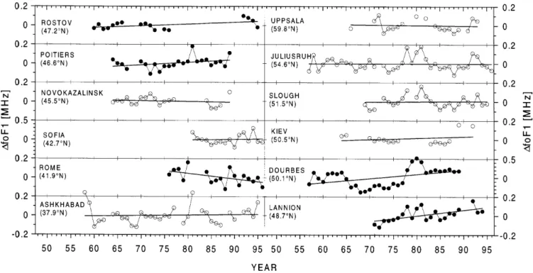
The peak electron density of the F1 layer, foF1, has been used for a trend analysis at F1 region heights near 170± 180 km. Unfortunately only values of 12 stations were available, 4 stations for the region east of 30° E and 8 stations in the western part of Europe. In Fig. 4 the trend results are therefore presented only in their dependence on latitude and not subdivided into di€erent longitudinal regions. The trends are in most cases positive (9 of 12 trends including 4 of 5 signi®cant trends) with a median value 0.001 MHz/year. In agree-ment with the results in the F2 region in the F1 layer the trends do not markedly depend on the latitude, but in contrast to the F2 layer in the F1 layer no marked di€erences could be found also for di€erent longitudinal regions. At longitudes west of 30° E 6 of 8 stations have positive trends, and at longitudes east of 30° E 3 of 4 trends are positive.

3.3 E region

The E region re¯ection height h¢E and the peak electron density foE have been used for trend analyses at E region heights (110±120 km). In Fig. 5 the results for h¢E are presented. Unfortunately only observations at 10 stations are available, and all of them are from the western part of Europe. From most of measurements negative trends were derived (8 of 10 including 5 of 6 signi®cant trends) with a median value )0.07 km/year. Also here the trends do not show a marked dependence on latitude.

In Fig. 6 the foE trends for 25 European stations are shown, separated again for two longitudinal regions west (upper part) and east of 30° E (lower part). The trends are relatively uniform, 22 of 25 trends (including 10 of 11 signi®cant trends) are positive. The median trend value is 0.0013 MHz/year. Marked longitudinal and latitudinal dependencies could not be found in the European E region investigated.

4 Discussion

As the ionospheric plasma parameters are markedly controlled by the solar activity it is necessary to remove this part carefully if derivation of long-term trends are required which are normally more than one order of magnitude smaller than the solar induced variations. In this study a linear dependence of the plasma parameters on solar as well as geomagnetic activity is adopted to describe the solar in¯uence. This model is very similar to a model used by Kane (1992) to get a better description of the hysteresis e€ect in foF2 observations. Kane (1992)

Fig. 1. Yearly trends of DhmF2 after elimination of the solar and geomagnetic in¯uences for European stations at longitudes west of 30°E (upper part) and at longitudes east of 30°E (lower part). Signi®cant trends (>90%) are marked by solid dots

only used the solar 10.7 cm radio ¯ux (F10.7) instead of the solar sunspot number R but also the geomagnetic Ap index. After Kouris et al. (1994) foF2 is slightly better correlated with solar activity if a quadratic relation is assumed (f (R, R2_{) ˆ a + bR + cR}2_{). This e€ect can} be seen in Fig. 7 where the monthly mean noon values (12 LT) of foF2, hmF2, foF1, foE, and h¢E from observations at Juliusruh between 1957 and 1996 are presented showing their dependence on solar activity. The data for January (crosses) and July (solid circles) are shown together with the linearly (complete lines) and quadratically ®tted curves (dashed). The di€erences between the linear and quadratic approximations are often very small but sometimes remarkable (e.g. hmF2 in July). The quality of the di€erent approximations of the solar-induced variations can be tested by correlation coecients between the observed data with the di€erent model results of these data. In Fig. 8 these correlation coecients are presented for foF2 and hmF2 data from Juliusruh for January and July dependent on local time. All correlation coecients are highly signi®cant, also for the parameters foF1 and foE (not shown here), although the correlation of h¢E with solar activity is markedly smaller. The di€erences between the correlation coe-cients for the same ionospheric parameter are very small. In most cases the correlation with the linear f (R) model (open circles in Fig. 8) is slightly smaller and the best correlations have been found sometimes for the f (R, Ap) values (crosses) and sometimes for the f (R, R2₎ values (solid circles). In Fig. 9 the trends in foF2 and hmF2 for Juliusruh are presented using di€erent models to remove the solar-induced variation. Here all data (all 24 h of all 12 months) have been used as in Figs. 1±6. The general agreement of the three di€erent curves of the DfoF2 and DhmF2 values in Fig. 9 is very good, indicating that the derived trends do not depend greatly on the model used to eliminate the solar-induced variation. In detail small di€erences may occur in the individual data, the general behaviour, however, is little in¯uenced by the choice of the model. In particular the f (R, R2) and the f (R, Ap) models give very similar results.

Independent of the model used the removal of the solar-induced variation requires a long data series. Therefore in this study nearly all data series investigated are longer than 20 y with only very few exceptions, as can be seen in Figs. 1±6.

The model calculations for an atmospheric green-house e€ect are normally carried out for a doubling of the greenhouse gases CO2and CH4. To compare these theoretical results with our experimental trend data it is necessary to take into account the real changes of these gases during the last 40 y, corresponding to the main interval of ionosonde observations which has been analysed here. After the recent IPCC report (Houghton et al., 1996) and Brasseur and de Rudder (1987) the atmospheric content of these gases has increased during the last 40 y for CO2by about 15%, CH4by about 44%, N2O by about 7% and for the CFCs and HCFCs partly by essentially higher rates (yearly increases between 0.5%). Taking into account the di€erent amounts of these greenhouse gases, for the total direct radiative forcing, after Houghton et al. (1996) an e€ective increase of the greenhouse gases of about 20% can be assumed for the last 40 y.

After the model calculations of Rishbeth (1990) and Rishbeth and Roble (1992) the F2 peak height hmF2 should be lowered by about 10±20 km if the greenhouse gases are doubled, corresponding to a lowering of about 2±4 km for the last 40 y. The median experimental trends derived in this study however, give a lowering of 7.2 km (at longitudes west of 30° E) or an increase of 7.6 km (at longitudes east of 30° E) for the last 40 y. Whereas the experimental lowering of hmF2 in the western part of Europe is only slightly stronger than the theoretically expected result, in the eastern part even the direction between predicted and observed trend values is contrary. Such a behavior of regional di€erences in the hmF2 trends has also been found by Ulich and Turunen (1997b) using data from ionosonde stations all around the world. It is dicult to decide if technical changes of the equipment or changes in the evaluating algorithm could be responsible for the considerable di€erences especially for the unexpected positive trends in the eastern part of Europe. Therefore, for three stations of this region the hmF2 trends are shown in Fig. 10 once again. Indeed there seem to be some discontinuities in the trends (marked by dotted vertical lines) which could be caused by technical changes, but nevertheless there remain large parts of the observations with positive trends. Therefore, the trends of individual stations may be partly in¯uenced by technical changes, but it seems to be impossible to argue that the positive trends in the eastern part of Europe and in other regions of the world as found by Ulich and Turunen (1997) are only caused by arti®cial changes.

Similar di€erences to those for hmF2 trends were also detected in the foF2 trends in Fig. 3. In the western part of Europe we detected a mean foF2 decrease during the last 40 y of about 0.1 MHz which is in relatively good agreement with the results of Rishbeth and Roble (1992) who predicted a lowering up to about 0.5 MHz for a doubling of the greenhouse gases. But in the eastern part

Fig. 2. hmF2 trend coecients dependent on longitude. Signi®cant trends are marked by solid dots. The solid lines represent the median values of all individual trends in the regions west or east of 30°E

of Europe an increase of about 0.06 MHz was detected in contrast to the predicted reduction of Rishbeth and Roble (1992). In general the di€erences between the foF2 trends in the western and eastern part of Europe qualitatively agree with the di€erences in the hmF2 trends, however the di€erences in the hmF2 trends seem to be more pronounced. The reason for these longitu-dinal di€erences are not yet known, but they are probably caused by the complex dynamics of the F2 region. The hmF2 and foF2 maps derived with the TIGCM by Rishbeth and Roble (1992) contain struc-tures which could be connected with di€erent regional trends of these F2 region parameters. However detailed

experimental and theoretical investigations are neces-sary in the future to reach a better understanding of trends in the F2 region dependent on latitude and longitude.

At lower heights (F1 and E regions) where dynamical processes are not so dominant as in the F2 layer latitudinal as well as longitudinal di€erences could not be detected. Using the median foF1 trend of 0.001 MHz/ year a mean foF1 increase of 0.04 MHz during the last 40 y was derived from the experimental results. Rishbeth and Roble (1992) derived, with their model calculations, an increase in the electron density near the peak height of the F1 layer between 5% and 50%, with a median value

Fig. 4. Same as Fig. 1, but for DfoF1 values and not subdivided into di€erent longitudinal regions

near 15% corresponding to a mean increase in foF1 up to about 8% for a doubling of the greenhouse gases. For typical foF1 values of 4±6 MHz an foF1 increase of 0.3± 0.5 MHz (or an increase of about 0.06±0.1 MHz for the last 40 y) can be expected from the modelling results. The agreement with the mean experimental trend value is quite reasonable, the median experimental trend is only smaller by a factor of about 2.

In the E region two parameters have been used for trend investigations, h¢E and foE (see Figs. 5 and 6). With the median trend value of -0.07 km/y we get a lowering of the E region by about 2.8 km during the last 40 y which is in the same order as predicted by Rishbeth (1990) for a doubling of the greenhouse gases. There-fore, the experimental value is higher than the predicted value by about a factor of 5. Using the mean foE trend of 0.0013 MHz/year a foE increase of about 0.05 MHz was observed during the last 40 y. After the model calculations of Rishbeth and Roble (1992) an increase of the electron density at E region heights of about 5%

(corresponding to an increase in foE by about 2.5%) is predicted for a doubling of the greenhouse gases. For typical foE values of 2±3 MHz an foE increase of about 0.05±0.08 MHz can be expected (or 0.01±0.02 MHz for the last 40 y). Also for this parameter the mean experimental trend value is slightly higher than the prediction. The observed foE increase is also in quali-tative agreement with trends of the ion ratio [NO+_]/ [O2+] obtained from mass spectrometer measurements by Danilov and Smirnova (1997). They found, for E region heights, a strong negative trend in [NO+_]/[O

2+] which causes a decreasing e€ective recombination coef-®cient (as the dissociative recombination coecient of the NO+ _{ions is about twice that of the O}

2+ions) and therefore an increase of the electron density at the E region peak height. The negative trend in [NO+_]/[O

2+] again is caused by the reduced NO density as expected after model calculations for increasing atmospheric greenhouse gases (Roble and Dickinson, 1989; Chakra-barty, 1997; Beig and Mitra, 1997).

(12 LT, January and July, 1957±1996) in relationship to solar sunspot number R ®tted by linear (complete lines) and quadratic curves (dashed)

Fig. 8. Correlation coecients between ex-perimental monthly median foF2 or hmF2 data (Juliusruh, January and July, 1957± 1996) and di€erent model values assuming a linear (open circles) or quadratic dependence on solar sunspot number R (solid circles) and for a twofold regression with R and geo-magnetic Ap values (crosses) in dependence on local time LT

5 Conclusions

Based on observations at 31 European ionosonde stations over the last 40 y long-term trends have been derived at di€erent ionospheric parameters of the E, F1 and F2 regions. In spite of marked di€erences between the results derived at single stations some common results could be found:

1. Technical changes of equipment or the evaluation algorithms used may partly in¯uence the trend results derived for individual stations. However the compar-ison of the results of many di€erent stations allows the derivation of representative (median) trends for the European region (5°W )70° E; 35°N - 70°N). 2. The trends in the E and F1 layers with lowering of

the E region height, h¢E, and increases of the peak electron densities, foE and foF1, do not depend on latitude and longitude and are in qualitative agree-ment with modelling results of the atmospheric greenhouse e€ect. The experimental mean trends are, however, stronger by a factor of 2..5 compared with the theoretical predictions for the E region and smaller by a factor of 2 with F1 region predictions. 3. The trends in the F2 region (hmF2 and foF2) do not depend on latitude but show marked di€erences for the longitudinal regions west or east of 30° E.

Whereas at longitudes west of 30° E the trends in hmF2 as well as foF2 are in general negative as expected after model calculations for an atmospheric greenhouse e€ect, the trends in the European region east of 30° E are in general positive. These longitu-dinal di€erences are more pronounced in the hmF2 data but could also be detected in the foF2 data. The cause of these regional di€erences which were also found by Ulich and Turunen (1997b) in world-wide hmF2 data is unknown at present and needs further investigations.

Acknowledgements. This work was partly supported by the Bundesministerium fuÈr Bildung, Wissenschaft, Forschung und Technologie (BMBF), Bonn, under contract 07VKV01/1.

Topical Editor D.Alcayde thanks J. Lastovicka and T.J. Fuller - Rowell for their help in evaluating this paper.

References

Beig, G., and A. P. Mitra, Atmospheric and ionospheric response to trace gas perturbations through the ice age to the next century in the middle atmosphere. Part I - chemical composition and thermal structure, J. Atmos. Solar-Terr. Phys. 59, 1245± 1259, 1997.

Bilitza, D., N. M. Sheikh, and R. Eyrig, A global model for the height of the F2-peak using M3000 values from the CCIR numerical map, Telecom J., 46, 549±553, 1979.

Brasseur, G., and A. de Rudder, The potential impact on atmospheric ozone and temperature of increasing trace gas concentrations, J. Geophys. Res., 92, 10903±10920, 1987. Fig. 9. Trends in foF2 and hmF2 values of Juliusruh after removing the

solar induced variation by a linear model f(R), a quadratic model f(R,R2_{) and a twofold linear model f(R, Ap) with the solar sunspot}

number and the geomagnetic Ap index

Fig. 10. Yearly trends of DhmF2 after elimination of the solar and geomagnetic in¯uences for three stations with sudden DhmF2 changes (near the dotted vertical lines) which could be caused by technical changes

Bremer, J., Ionospheric trends in mid-latitudes as a possible indicator of the atmospheric greenhouse e€ect, J. Atmos. Terr. Phys., 54, 1505±1511, 1992.

Bremer. J., Some additional results of long-term trends in vertical-incidence ionosonde data, Paper 4051, presented at the COST 251 Meeting, Prague, 1996.

Bremer, J., Long-term trends in the meso- and thermosphere, Adv. Space Res., 20, (11), 2075±2083, 1997a.

Bremer, J., Long-term trends in the ionospheric E- and F- regions over Europe, Paper 6306, presented at the COST 251 Meeting, LinkoÈping, 1997b.

Chakrabarty, D. K., Mesopause scenario on doubling of CO2, Adv.

Space Res, 20, (11), 2117±2125, 1997.

Danilov, A. D., and N. V. Smirnova, Long-term trends in the ion composition in the E region (in Russian), Geomagn. Aeron., 37, (4), 35±40, 1997.

Houghton, J. T., L. G. Meira Filho, B. A. Callander, N. Harris, A. Kattenberg, and K. Maskell, Climate Change 1995, Contribution of WGI to the Second Assessment Report of the Intergovern-mental Panel on Climate Change, Cambridge University Press, Cambridge, UK, 1996.

Kane, R. P., Solar cycle variation of foF2, J.Atmos. Terr. Phys. 54, 1201±1205, 1992.

Kouris, S. S., P. A. Bradley, and I. K. Nissopoulos, The relation-ships for foF2 and M(3000)F2 versus R12, Numerical mapping

and modelling and their application to PRIME, Scienti®c Report, COST Document: COST238TD(94)010, Eindhoven, 155±167, 1994.

Rishbeth, H., A greenhouse e€ect in the ionosphere?, Planet. Space Sci., 38, 945±948, 1990.

Rishbeth, H., and R. G. Roble, Cooling of the upper atmosphere by enhanced greenhouse gases ± Modelling of thermospheric and ionospheric e€ects, Planet. Space Sci., 40, 1011±1026, 1992. Roble, R. G., and R. E. Dickinson, How will changes in carbon

dioxide and methane modify the mean structure of the mesosphere and thermosphere?, Geophys. Res. Lett., 16, 1441± 1444, 1989.

Shimazaki, T., World wide daily variations in the height of the maximum electron density in the ionospheric F2 layer, J. Radio Res. Labs., Japan, 2, 85±97, 1955.

Taubenheim, J., Statistische Auswertung geophysikalischer und meteorologischer Daten, Akad. Verlagsgesell. Geest and Portig K.-G., Leipzig, 1969.

Ulich, T. and E. Turunen, Evidence for long-term cooling of the upper atmosphere, Geophys. Res. Lett., 24, 1103±1106, 1997a. Ulich, T., and E. Turunen, Long-term behavviour of ionospheric F2

layer peak height on a global scale, Paper presented at Session 2.18 of the 8th_{Scienti®c Assembly of IAGA, Uppsala, 1997b.}