HAL Id: hal-01862664
https://hal.archives-ouvertes.fr/hal-01862664
Submitted on 27 Aug 2018
HAL is a multi-disciplinary open access
archive for the deposit and dissemination of sci-entific research documents, whether they are pub-lished or not. The documents may come from teaching and research institutions in France or
L’archive ouverte pluridisciplinaire HAL, est destinée au dépôt et à la diffusion de documents scientifiques de niveau recherche, publiés ou non, émanant des établissements d’enseignement et de recherche français ou étrangers, des laboratoires
Computer-aided placement of air quality sensors using
adjoint framework and sensor features to localize indoor
source emission
Julien Waeytens, Sara Sadr
To cite this version:
Julien Waeytens, Sara Sadr. Computer-aided placement of air quality sensors using adjoint framework and sensor features to localize indoor source emission. Building and Environment, Elsevier, 2018, 144, pp.184-193. �10.1016/j.buildenv.2018.08.012�. �hal-01862664�
Computer-aided placement of air quality sensors using
1
adjoint framework and sensor features to localize indoor
2
source emission
3
Julien Waeytensa,b,∗, Sara Sadra
4
aUniversit´e Paris-Est, IFSTTAR, 14-20 bd Newton, Marne-la-Vall´ee, 77447, France 5
b
Efficacity, 14-20 bd Newton, Marne-la-Vall´ee, 77447, France 6
Abstract
7
With the improvement in sensor technologies, air quality is increasingly
be-8
ing monitored. Two major factors in obtaining relevant information are
9
the optimal placement and the number of air quality sensors. Moreover,
10
in cases of poor air quality, the information of the pollution level given by
11
the deployed sensors is not sufficient. An advanced understanding of the
12
data is required to precisely identify the source pollution and thus propose
13
effective solutions. In this article, a virtual testing strategy based on
com-14
putational fluid dynamics (CFD) is presented for the optimal placement of
15
indoor air quality sensors. We determine the placement of sensors in view
16
of localizing the maximum of sources emitting on the indoor environment
17
surfaces. Therefore, an adjoint framework is used to obtain the observable
18
region associated with a given sensor position. The proposed method takes
19
into account technical sensor features, such as the limit of detection (LOD).
20
Two applications are studied: a simple 2D case and a real 3D room. In
21
these examples, we first show that reducing the LOD of the sensors by one
22
order of magnitude can increase the observable area by more than 50%.
23
∗
Corresponding author: E-mail: [email protected] (J. Waeytens), Ph: +33 1
81 66 84 53, Fax: +33 1 81 66 80 01, Postal address: Cit´e Descartes, 14-20 bd Newton,
Then, we note that one-fourth of the potential sensor placements observe almost nothing and that 80% of the potential sensor placements have an
ob-servable area two times smaller than the optimal sensor position determined by the proposed CFD-based strategy.
Keywords: sensor placement, computational fluid dynamics, adjoint
24
problem, source emission, sensor detection limit, indoor air quality
25
1. Introduction
26
According to a survey conducted in 2015 by the French Ministry of
27
Ecological Transition, air pollution is the second environmental concern of
28
French people, just after climate change. As people spend approximately
29
80% of their time in indoor environments, increasing attention has been
30
focused on indoor air quality (IAQ). Volatile organic compounds (VOCs)
31
are characteristic chemical species present in indoor environments. Several
32
studies have shown that the concentration of VOCs can be higher in indoor
33
locations, such as early childhood education facilities [1], schools [2],
univer-34
sities [3], office buildings [4] and homes [5], compared to the concentrations
35
outside. As reported in [6], VOCs in indoor environments can come from
36
the outdoor air via ventilation and from indoor sources. There are a wide
37
range of indoor sources, e.g. combustion, smoking, building materials,
of-38
fice machines, furnishings, paints, termiticides and cleaning products. As
39
permanent and occasional exposure, even at low VOC levels, has an impact
40
on human health [7], it is important to monitor indoor air quality and to
41
precisely localize sources to propose an appropriate action plan to improve
42
air quality. The monitoring of air quality is facilitated by the improvement
43
in sensor technologies, notably nanotechnologies. Hence, the gas sensors
44
become cheaper, smaller, more sensitive, less energy-consuming, etc... To
get more details on low-cost sensors for air quality purposes, the reader can
46
refer to the review article [8]. The localization of VOC sources can also
47
be useful for the preservation of cultural heritage, notably artwork, and for
48
structural health monitoring purposes. In most regions of France, the
pres-49
ence of woodborers, such as termites, has harmful effects on the safety of
50
structures. The VOC chemical signature of termites can be used for their
51
early detection and localization, which will provide the ability to limit the
52
use of termiticides and to preserve the structure.
53
54
To efficiently monitor air quality, the number of sensors and their
po-55
sitioning are crucial. In most measurement campaigns, the gas sensors are
56
placed in an empirical way. For example, in a room, an air quality sensor is
57
usually positioned at the breathing zone height or approximately 0.5m from
58
the ceiling in the middle of the room. Unfortunately, this placement does
59
not take into account the characteristics of the room, i.e. the geometry and
60
the ventilation. As a consequence, bad sensor placement may lead to the
61
nondetection of some sources. To well-position gas sensors, we can take
ad-62
vantage of numerical simulations derived from physical models. In indoor air
63
quality applications, the gas concentration can be predicted using multizone
64
[9; 10; 11; 12] and CFD [9; 13; 14] models. Multizone techniques, which
pro-65
vide the time evolution of the averaged concentration in each zone as output,
66
are easy to use and run on a standard laptop. Nevertheless, they consider
67
strong hypotheses, such as a well-mixed concentration. With the ongoing
68
improvement of computers and numerical methods, CFD approaches
ap-69
pear to be promising for the prediction of indoor air quality and for optimal
70
sensor placement. In fact, CFD provides a fine description of the spatial
71
concentration in the indoor environment, but the computations are time
consuming. A good compromise to study the indoor air quality of an entire
73
building would be to couple multizone and CFD models, as proposed in [15].
74
To the best of the authors’ knowledge, few publications have addressed the
75
optimal placement of gas sensors for IAQ applications. The design of an
op-76
timal sensor network, i.e. the number and positioning of sensors, has been
77
studied in greater depth in terms of chemical and biological warfare (CBW)
78
and transmission of infectious diseases (TID). The sensor positions are
cho-79
sen to early detect and localize indoor contamination. Different methods
80
aim to maximize the coverage area of sensors and to minimize the response
81
time for various sets of release scenarios. In [16], the sensor coverage area is
82
evaluated using CFD and an adjoint advection-diffusion equation, whereas
83
physical model-free approaches based on a dynamical systems approach are
84
preferred in [17]. Note that the adjoint framework is a useful numerical tool
85
for various applications. First, it provides, at a low computational cost,
86
the functional gradient and the Hessian matrix involved in inverse
calcula-87
tions to update the parameters of fluid mechanics models [18; 19] and to
88
reconstruct the concentration fields [20; 21; 22]. Additionally, it is used in
89
sensitivity analyses to study the influence of physical model parameters on
90
a quantity of interest [23; 24]. The adjoint framework is also considered
91
for estimating the modeling or discretization error on a quantity of interest
92
[25; 26; 27].
93
94
Once the positions of the sensors are fixed, knowledge of the
concentra-95
tion given by the deployed sensors is not sufficient for proposing efficient
96
solutions for indoor air quality improvement or for localizing woodborers.
97
One needs to localize and to quantify the source emissions. To achieve this
98
purpose, two families of methods can be found in the literature, i.e.
driven methods and physical model-based methods. Direct measurements
100
of the source emissions on different surfaces of the environment (furniture,
101
wall, floor, door, etc.) can be planned using innovative sensors, such as fibers
102
placed in a specific device for on-site emission control [28; 9]. This method
103
enables accurate in situ quantification of the source emissions for building
104
materials and furniture, but it requires a large number of sensor devices.
105
Another data-driven method to evaluate source emissions is indirect
mea-106
surements. In contrast to the previous methods, the air quality sensors are
107
placed in the room volume and not directly on a surface. Databases of the
108
chemical signatures of sources and a priori information of the studied
envi-109
ronment collected via questionnaire, including the type and the age of the
110
building materials, renovations, cleaning products and ventilation, are
com-111
monly considered in these methods. Finally, the sensor outputs associated
112
with various chemical compounds are analyzed via statistical tools, such
113
as proper component analysis and linear regression, to identify the source
114
emissions [4; 5; 29; 30]. In practice, the chemical compounds emitted by
115
some items in the studied environment may not be referenced in a database.
116
Consequently, these methods may only approximately identify the sources.
117
Physical model-based approaches via inverse modeling techniques can also
118
be valuable for the localization and the quantification of source emissions.
119
In general, inverse problems that couple model and sensor outputs are not
120
well-posed in the sense of Hadamard, i.e the existence, uniqueness and
non-121
high sensitivity of the solution to the sensor outputs. To address this issue,
122
a sufficient number of well-positioned sensors is required, and regularization
123
must be considered in the mathematical formulation of the inverse problem.
124
In deterministic settings, Tikhonov regularization is commonly considered
125
and consists of adding penalization terms to the data misfit functional, as
discussed in [15; 31] for convective-diffusive transport source inversion. In
127
probabilistic inversion formalism, notably Bayesian model updating, which
128
was applied in [32] for CO2 regional source estimations, the model
parame-129
ter probability distributions are interesting on two counts. They ensure the
130
problem regularization and provide a confidence interval on the identified
131
source emissions. Nevertheless, probabilistic inversions can be much more
132
time consuming than deterministic ones. Finally, the adjoint framework,
133
previously mentioned for the optimal placement of sensors, can also be used
134
for source localization, as shown in [33; 15].
135
136
In the present article, we propose a virtual testing strategy, taking into
137
account the specificities of the indoor environment (geometry and
venti-138
lation) via CFD and gas sensor features (limit of detection), to efficiently
139
select the number and positions of sensors to localize indoor sources. We
de-140
fine the “optimal sensor placement” as the combination of gas sensors that
141
maximizes the coverage area. The authors showed in previous works [21]
142
that the sensor observable area can be computed at a reasonable cost using
143
the adjoint framework. Herein, we emphasize that the coverage area can be
144
increased not only by adding sensors but also by using sensors with a lower
145
limit of detection. The rest of this article is organized as follows. In Section
146
2.1, a physical direct model to predict the gas dispersion is presented. Then,
147
we define the adjoint equations in Section 2.2 and introduce a new
adjoint-148
based criterion integrating sensor features to evaluate the observable area of
149
potential sensor positions in Section 2.3. An overview of the optimal sensor
150
placement strategy is given in Section 2.4, and it is applied to a 2D case and
151
a real 3D room in the last section.
2. Materials & Methods
153
2.1. Simulation of pollutant propagation - Direct problem
154
To predict the dispersion of gas, advection-diffusion-reaction models are
155
commonly used [9; 13; 14]. As a first step, we consider non-reactive gases,
156
i.e. reaction phenomena are not modeled. Hence, the cartography of the
157
gas concentration in a two- or three-dimensional space domain Ω is obtained
158
from the advection-diffusion model. Four types of boundaries can be
dis-159
tinguished. A boundary presenting a known prescribed concentration Cp
160
is denoted ∂pΩ. Potential pollution emissions, to be precisely located by
161
the optimal placement of gas sensors, are on the boundary ∂uΩ, whereas a
162
boundary that does not present source emission is ∂nΩ. Lastly, ∂oΩ denotes
163
the outgoing flow boundary.
164
165
The pollutant concentration C(x, t) in the domain Ω ⊂ Rn, n ∈ {2, 3}
166
can be obtained by solving the unsteady advection-diffusion model, which
167
is also called the “direct problem”,
168 ∂C ∂t(x, t) + v(x, t) · ∇C(x, t) − ν(x, t)∆C(x, t) = 0 in Ω × [0, T ] C(x, t) = Cp(x, t) on ∂pΩ × [0, T ] C(x, t) = Cu(x, t) on ∂uΩ × [0, T ] ∇C(x, t) · n = 0 on ∂nΩ × [0, T ] ∇C(x, t) · n = 0 on ∂oΩ × [0, T ] C(x, t = 0) = C0(x) in Ω (1)
In Eq. (1), v is the flow velocity, ν denotes the diffusion parameter, which is
169
the sum of the molecular and turbulent diffusion, and n denotes the outside
normal vector to the surface.
171
172
When the flow and the source emission can be considered stationary with
173
respect to the monitoring time, the concentration field C(x) can be obtained
174
at a lower computation cost using a steady advection-diffusion model
175 v(x) · ∇C(x) − ν(x)∆C(x) = 0 in Ω C(x) = Cp(x) on ∂pΩ C(x) = Cu(x) on ∂uΩ ∇C(x) · n = 0 on ∂nΩ ∇C(x) · n = 0 on ∂oΩ. (2)
For example, Eq. (2) can be used to model the dispersion of moisture or
176
woodborers emissions during a measurement campaign under mastered air
177
flow conditions, e.g. when the indoor occupants have left. In the following,
178
we limit our study to stationary cases.
179
2.2. Sensitivity area of a gas sensor - Adjoint problem
180
Physically, the solution of the adjoint problem corresponds to a
sensitiv-181
ity function in terms of a quantity of interest. Hence, to obtain the sensor
182
observable area, we choose the gas concentration at the sensor location xs
183
as the quantity of interest. It is given by
184
J = Z
Ω
fs(x − xs)C(x)dΩ (3)
where fs is a space function to extract the gas concentration at the sensor
185
location xs. In practice, we can take:
186 fs(x − xs) = 1/|Ωs| for x ∈ Ωs 0 elsewhere. (4)
The domain Ωs is a sphere of radius Rs centered at the sensor location xs.
187
188
From the quantity of interest, we introduce the adjoint problem (5) and
189
compute its numerical solution ˜C.
190 −v(x) · ∇ ˜C(x) − ν(x)∆ ˜C(x) = fs(x − xs) in Ω ˜ C(x) = 0 on ∂pΩ ˜ C(x) = 0 on ∂uΩ ∇ ˜C(x) · n = 0 on ∂nΩ ν∇ ˜C(x) · n + v(x) · n ˜C(x) = 0 on ∂oΩ (5)
Note that the adjoint problem (5) is a backward-advection-diffusion problem
191
with a source emission located at the sensor position. This adjoint problem
192
can be solved with the same CFD software as that used for the direct
prob-193
lem. For greater detail on the derivation of the adjoint problem, the reader
194
can refer to [21].
195
2.3. Computation of sensor observable area - A new adjoint-based criterion
196
After defining the adjoint problem, we propose an adjoint-based criterion
197
(6) that takes into account the sensor features, i.e., the LOD of the gas
198
sensor, in view of obtaining the sensor observable area.
199 |∇J |As S dIm > 1 (6) where: 200
• J (resp., ∇J ) is the functional (resp., functional gradient) associated
201
with the gas concentration at the sensor location xsdefined in Eq. (3)
202
• As is the minimum source area expected to be localized
• S is the order of magnitude of the source emission
204
• dIm is the limit of detection of the gas sensor
205
The sensitivity of the gas concentration at the sensor location xs to the
206
surface source emissions, which corresponds to the functional gradient ∇J ,
207
can be evaluated using the adjoint framework. Following the method in [21],
208
we can show that:
209
∇J (x) = ν(x)∇ ˜C(x) · n (7)
where n denotes the unit outer normal vector along the surface.
210
211
In summary, the observable area of a gas sensor located at a given
posi-212
tion xs can be numerically predicted by
213
x ∈ ∂uΩ such that |ν(x)∇ ˜C(x) · n| As S
dIm
> 1. (8)
Let us physically interpret the different terms in the proposed criterion
214
(8). The first part |∇J (x)| takes into account the sensor position xs and
215
gives the sensitivity map of the gas sensor output to the surface source
emis-216
sion. It is numerically obtained from the solution ˜C of the adjoint problem
217
defined in Eqs. (5). In [21], we proved that a null value of |ν(x)∇ ˜C(x) · n|
218
on a boundary ∂bΩ ⊂ ∂uΩ implies that potential source emissions on ∂bΩ
219
cannot be detected by a sensor at the position xs.
220
The new contribution in this article concerns the next two terms. The
sec-221
ond term As× S relies on a priori information of the source emissions that
222
are expected to be detected. If we are interested in emissions on large
sur-223
faces, such as painted walls, Asshould be approximately a few tens of square
224
meters. By contrast, if we are interested in emissions on small surfaces, such
225
as furniture, As should be approximately one square meter. A small value
of As, i.e. less than one square meter, can also be useful for the early
de-227
tection of termites. The order of magnitude of potential emissions is taken
228
into account with the parameter S. For formaldehyde furniture emission it
229
can be higher than 1ppm [34] whereas it is a hundred times lower for VOCs
230
emitted by molds [35]. In the proposed criterion (8), the observable area for
231
a given positioned sensor depends on the product As× S. Hence, the higher
232
this product is, the larger the observable area.
233
Lastly, the sensor detection limit, depending on technology features,
cor-234
responds to the third term in the proposed criterion (8). In the Results
235
Section, we show how the observable area increases as the limit of detection
236
of the sensors decreases.
237
2.4. Outline of the virtual testing strategy for the optimal placement of air
238
quality sensors
239
This section aims to present the steps in computer-aided sensor
place-240
ment. The process is summarized in Figure 1.
241
Numerical Mock-Up
Air Flow map
List of nt sensor positions Number nm of desired sensor Source Emissions Characteristics Sensor Technology Features DATABASE OF ADJOINT SOLUTIONS OPTIMAL PLACEMENT OF 1st SENSOR OPTIMAL PLACEMENT OF 2nd SENSOR OPTIMAL PLACEMENT OF nmth SENSOR Optimal placement of nm sensors
Figure 1: Architecture of the computer-aided method for the optimal placement of air quality sensors
The proposed strategy necessitates a mock-up of the studied environment
242
and a fine description of the air flow. The air flow map can be obtained from
243
experiments, empirical models or computational fluid dynamics. Let us
em-244
phasize that [22] previously pointed out that a rough approximation of the
245
real flow can lead to a non-representative concentration simulation. Thus,
246
special attention must be given to obtaining the air flow map; otherwise,
247
the proposed placement of gas sensors can be incorrect. After defining a
248
list of nt potential sensor positions, we solve the adjoint problem (5)
asso-249
ciated with each sensor position. All the nt adjoint solutions are stored in
250
a database. Note that this step is fully parallelizable and is performed only
251
once in a off-line stage.
252
In the proposed virtual testing strategy, the observable area is computed for
253
the nt sensor positions. As shown in the previous section, the observable
254
area is obtained from the adjoint-based observable criterion (8). In addition
255
to the adjoint solution, a priori information of the sensor technology is also
256
required, i.e. the limit of detection dIm of the sensor and the source to be
257
localized, i.e. the orders of magnitude of area As and level S of the source
258
emissions. Lastly, the optimal placement corresponds to the one with the
259
largest observable area. When the number nm of desired sensors is strictly
260
greater than one, the optimal placement is performed in a hierarchical
man-261
ner. We start by optimally placing the first sensor and fix its position; then,
262
we seek the optimal placement of the second sensor and fix its position,
263
and so on. As practical outputs for the users, the computer-aided method
264
provides, as a visualization on the numerical mock-up, the observable area
265
of each selected sensor position and the coverage area in square meters for
266
each sensor and for the combination of all nm sensors.
3. Results
268
3.1. Application 1 - 2D simple problem
269
To gain a better understanding, let us first consider a 2D academic
prob-270
lem (see Figure 2). The 2D domain Ω is a square with 10 m sides, and the
271
flow V is uniform. The velocity amplitude (resp. the velocity orientation
272
angle) is 1m/s (resp., 27o), and the diffusion parameter ν is 2.2 × 10⁻²m2/s
273
which corresponds to the order of magnitude of the turbulent diffusion. As
274
introduced in Section 2.1, ∂oΩ denotes the outgoing flow boundary. In this
275
example, we aim to optimally place gas sensors to localize and quantify
276
sources coming from the boundary ∂uΩ. We focus on the detection of a
277
source emitting on an area greater than 1m on ∂uΩ and whose order of
278
magnitude of the amplitude is approximately 100ppm. From this
informa-279
tion, we take As = 1m and S = 100ppm in the observable criterion (8).
280
Moreover, in the domain Ω, gas sensors can be placed at a limited number
281
of positions. The sixteen potential sensor positions are shown in Figure 2.
282
10 m
10 m
Figure 2: Geometry of the 2D problem (left) and potential positions of the gas sensor (right)
In the followings, firstly the influence of the LOD of the gas sensor on
the observable area is studied for a unique given sensor. Then, the virtual
284
testing strategy is illustrated to optimally place several sensors.
285
3.1.1. Influence of the LOD on the observable area for a given sensor
posi-286
tion
287
In this section, we consider a given sensor position, that is, Sensor #3
288
(see Figure 2). The objective is to evaluate its observable area for different
289
LODs of the gas sensor. We use the proposed adjoint-based criterion (8).
290
First, one needs to solve the adjoint problem defined in Eq. (5), which
291
corresponds to a backpropagation of a pollutant emitted at Sensor location
292
#3 (see Figure 3). Then, from the adjoint solution ˜C and the LOD dIm, we
293
compute the criterion (8) and deduce the observable area associated with
294
the considered sensor. In Figure 3, we present the adjoint field ˜C and the
295
observable area of Sensor #3 for two different LODs: 10ppm and 0.1ppm.
296
For the considered flow, source emissions on the bottom edge cannot be
297
detected by Sensor #3. The observable area is located around the middle
298
of the left edge. Its precise position along the left edge is 4.9m ± 1.1m for
299
an LOD of 10ppm and 4.9m ± 2.2m for an LOD of 0.1ppm.
300
The evolution of the observable area for a wide range of LODs is
pre-301
sented in Figure 4. As expected, a reduction in the LOD leads to an increase
302
in the observable area. The observable area for Sensor #3 is one and a half
303
times larger (resp. two times larger) when using a gas sensor with a 1ppm
304
LOD (resp., 0.1ppm LOD) than one with a 10ppm LOD. In summary, this
305
study shows that the LOD of the gas sensor has a strong impact on the
ob-306
servable area for detecting source emissions. Consequently, the LOD must
307
be considered in the optimal placement strategies of air quality sensors.
308
S3
-V
Observable Area LOD: 10ppm Observable Area LOD: 0.1ppm Area A Area B Area CFigure 3: Adjoint problem solution ˜C associated with Sensor #3 and its observable area
for an LOD of 10 ppm and 0.1 ppm - Definition of Source Areas A, B, C for numerical validation of the observable criterion
0 1 2 3 4 5 6 7 0,001 0,01 0,1 1 10 LOD (ppm) +55% +130% +100% +160% Observable Area (m)
Figure 4: Observable Area of Sensor 3 as a function of the LOD - The observable area for an LOD of 0.1ppm is 100% larger than that with an LOD of 10ppm
On the basis of the adjoint-based criterion (8), we were able to
eval-310
uate the observable area associated with a given sensor position. Let us
311
numerically validate this observable criterion. Sensor position #3 is still
312
considered, and three source locations are defined on the left edge of the 2D
domain (see Figure 3). The different sources are 1 meter in length, and their
314
amplitude is 100ppm. As predicted by the proposed virtual testing strategy,
315
a source in Area A can be detected by the sensor with both LODs (0.1ppm
316
and 10ppm), a source emitted in Area B can be detected only by the sensor
317
with an LOD of 0.1ppm, and neither the 0.1ppm LOD sensor nor the 10ppm
318
LOD sensor can detect a source in Area C. For each source, we simulate
319
the associated gas dispersion by solving the direct advection-diffusion
equa-320
tions (2) and obtain the gas concentration at Sensor position #3. From this
321
concentration, we can verify whether the source is detected by the sensors
322
with an LOD of 0.1ppm or 10ppm. In Table 1, the results show that the
323
sensor observable area is well predicted by the adjoint-based criterion (8).
324
A 100ppm source emitted in Area B leads to a gas concentration of 3.27ppm
325
at Sensor position #3. This concentration can be detected by the 0.1ppm
326
LOD sensor but not by the 10ppm LOD sensor. This result is in agreement
327
with the predicted observable area shown in Figure 3.
328
Source detected by the sensor ?
Source location Concentration (Y: Yes,N: No)
at sensor position #3 0.1ppm LOD 10ppm LOD
Area A (4.9m ± 0.5m) 56.06ppm Y Y
Area B (3.3m ± 0.5m) 3.27ppm Y N
Area C (2.2m ± 0.5m) 0.04ppm N N
Table 1: Numerical validation of the adjoint-based observable criterion - Concentration at Sensor position #3 simulated for different source locations and verification of the source detection for a 0.1ppm LOD sensor and a 10ppm LOD sensor
3.1.2. Optimal placement of gas sensors considering a fixed LOD
329
The optimal placement of the gas sensors is achieved using the virtual
330
testing strategy presented in Section 2.4. First, we determine the optimal
331
placement of the first sensor. Hence, for each sensor position, the associated
332
adjoint problem is solved and saved in a database. The use of the adjoint
333
solutions and the LOD in criterion (8) enable the evaluation of the observable
334
area of each sensor. Herein, the LOD is fixed to 10ppm. The sensor position
335
with the largest observable area is selected as the “optimal placement”.
336
The observable area associated with each sensor is summarized in Figure 5.
337
Note that the sum of the observable areas on the bottom and left edges
338
corresponds to the total observable area on the boundary ∂uΩ. We observe
339
that Sensors #1 to #11 can detect a source emission only on the left edge,
340
whereas Sensors #12 and #14 are able to detect a source emission located
341
in the lower-left corner of the domain involving the left and bottom edges.
342
Among the 16 potential positions, 13 positions have a total observable area
343
between 1 and 2.5m, and only 3 positions give an observable area larger
344
than 3m. Sensor #12, which has a total observable area slightly larger than
345
those of Sensor #15 and Sensor #16, is selected as the optimal placement.
346
As mentioned in Figure 1, the placement of several air quality sensors
347
is performed in a hierarchical manner. After finding the optimal placement
348
of the first sensor, we fix this sensor and determine the optimal placement
349
of the second sensor, and so on. Previously, Sensor #12 was determined
350
as the optimal placement for the first sensor. To determine the optimal
351
placement of several sensors, we evaluate the observable areas (see Figure
352
5) and select the sensor combination with the highest total observable area.
353
The combination of Sensors #12 and #16 gives the highest total observable
12-1 12-2 12-3 12-4 12-5 12-6 12-7 12-8 12-9 12-10 12-11 12-13 12-14 12-15 12-16 12-16-1 12-16-2 12-16-3 12-16-4 12-16-5 12-16-6 12-16-7 12-16-8 12-16-9 12-16-10 12-16-11 12-16-13 12-16-14 12-16-15 12-16-4-1 12-16-4-2 12-16-4-3 12-16-4-5 12-16-4-6 12-16-4-7 12-16-4-8 12-16-4-9 12-16-4-10 12-16-4-11 12-16-4-13 12-16-4-14 12-16-4-15 1 2 3 4 5 6 7 8 9 10 11 12 13 14 15 16 0,00 0,50 1,00 1,50 2,00 2,50 3,00 3,50 4,00 4,50 5,00 5,50 6,00 0,00 0,50 1,00 1,50 2,00 2,50 3,00 3,50 4,00 4,50 5,00 5,50 6,00 1m 2m 3m 4m 5m 6m 7m 8m 9m 10m 11m OB SER V
ABLE AREA ON LEF
T EDGE
(m)
OBSERVABLE AREA ON BOTTOM EDGE (m)
Figure 5: Optimal placement (red rectangles) in the 2D domain of several sensors of with an LOD of 10ppm - Observable Areas - Isovalues of the total observable area are represented as solid lines
area, that is, 6.5m. We can see that adding Sensor #16 improves the
ob-355
servable area on only the bottom edge, increasing from 2m to 5.5m. The
356
observable area on the left edge is increased by the optimal placement of
357
three sensors, i.e., Sensors #12, #16 and #4. We note that the the total
358
observable area is three times larger for the optimal placement of four
sen-359
sors (#12, #16, #4, #2) than for the optimal placement of a single sensor
360
#12.
361
3.1.3. Optimal placement of several sensors considering different LOD
362
In Section 3.1.1, we showed that the LOD has a significant influence on
363
the observable area for detecting source emissions. As a consequence, two
364
factors can be investigated to improve the observable area: the number of
365
gas sensors and the LOD. In this section, we study the optimal placement
of several sensors in the 2D domain when considering sensors with an LOD
367
of either 10ppm or 1ppm. The results are summarized in Figure 6. We
ob-368
serve that the optimal positions of gas sensors may differ according to the
369
LOD. At a 10ppm LOD, Sensor #12 is selected as optimal, whereas Sensor
370
#16 is optimal at a 1ppm LOD. Note that Sensor #16 with a 1ppm LOD
371
has a total observable area that is approximately twice the size of that of
372
Sensor #12 with a 10ppm LOD. To reach a total observable area of 9m, we
373
can either use two Sensors (#16, #14) with a 1ppm LOD or three Sensors
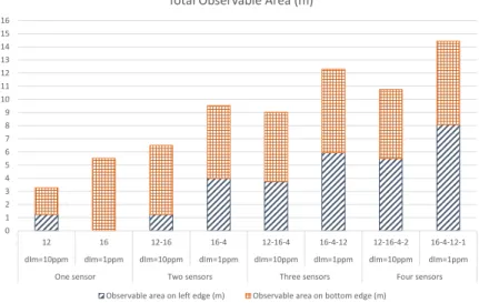
374 (#12, #16, #4) with a 10ppm LOD. 375 376 0 1 2 3 4 5 6 7 8 9 10 11 12 13 14 15 16 12 16 12-16 16-4 12-16-4 16-4-12 12-16-4-2 16-4-12-1
dIm=10ppm dIm=1ppm dIm=10ppm dIm=1ppm dIm=10ppm dIm=1ppm dIm=10ppm dIm=1ppm
One sensor Two sensors Three sensors Four sensors
Total Observable Area (m)
Observable area on left edge (m) Observable area on bottom edge (m)
Figure 6: Evolution of the observable area as a function of the number of sensors and the LOD (10ppm and 1ppm)
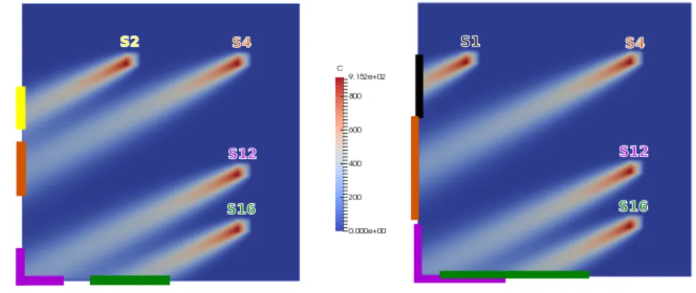
In Figure 7, we present the observable area associated with the optimal
377
placement of four gas sensors with LODs of either 10ppm or 1ppm. The
cov-378
erage is disparate on ∂uΩ for a 10ppm LOD while it is widespread for a 1ppm
LOD. Nevertheless, for both cases, source emissions cannot be detected in
380
the upper part of the left edge and the right part of the bottom edge due to
381
the considered flow V and the distribution of the sixteen potential sensor
382
positions. Lastly, for the optimal placement with 1ppm LOD gas sensors,
383
the observable area of some sensors overlaps, notably Sensors #12 and #16.
384
Thus, a source emitted in the overlapped region would be detected by both
385 Sensors #12 and #16. 386 S1 S4 S12 S16 S4 S12 S16 S2
Figure 7: Map of the observable area for the optimal placement of 4 sensors with LODs of 10 ppm (left) and of 1 ppm (right)
3.2. Application 2 - 3D laboratory room
387
In this section, we illustrate the computer-aided method for the optimal
388
placement of gas sensors in a real 3D laboratory room, including furniture
389
and ventilation systems, located at the IFSTTAR research institute. The
390
dimensions of the room are 5.9m × 6.2m × 4.2m, which correspond to a
391
volume of 150m3. As mentioned in Figure 1, we first need a numerical
mock-392
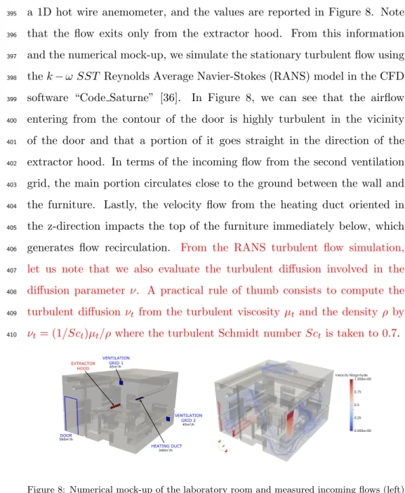
up and indoor air flow map (see Figure 8). For that, the incoming flows from
393
the heating duct, the two ventilation grids and the door were measured using
a 1D hot wire anemometer, and the values are reported in Figure 8. Note
395
that the flow exits only from the extractor hood. From this information
396
and the numerical mock-up, we simulate the stationary turbulent flow using
397
the k − ω SST Reynolds Average Navier-Stokes (RANS) model in the CFD
398
software “Code Saturne” [36]. In Figure 8, we can see that the airflow
399
entering from the contour of the door is highly turbulent in the vicinity
400
of the door and that a portion of it goes straight in the direction of the
401
extractor hood. In terms of the incoming flow from the second ventilation
402
grid, the main portion circulates close to the ground between the wall and
403
the furniture. Lastly, the velocity flow from the heating duct oriented in
404
the z-direction impacts the top of the furniture immediately below, which
405
generates flow recirculation. From the RANS turbulent flow simulation,
406
let us note that we also evaluate the turbulent diffusion involved in the
407
diffusion parameter ν. A practical rule of thumb consists to compute the
408
turbulent diffusion νt from the turbulent viscosity µt and the density ρ by
409
νt= (1/Sct)µt/ρ where the turbulent Schmidt number Sct is taken to 0.7.
410 DOOR HEATING DUCT VENTILATION GRID 1 VENTILATION GRID 2 EXTRACTOR HOOD 340m3/h 560m3/h 65m3/h 45m3/h
Figure 8: Numerical mock-up of the laboratory room and measured incoming flows (left) - Flow simulated by CFD software (right)
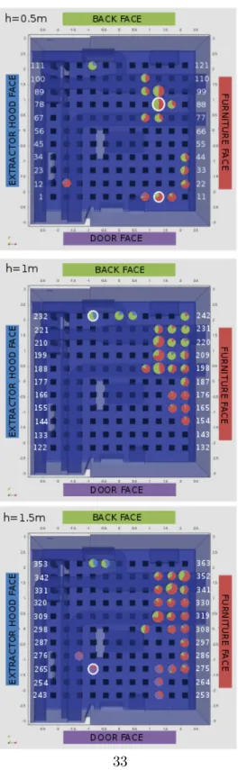
In the laboratory room, the potential sensor positions presented in
ure 10 are equally distributed every 50cm at three heights above the ground,
412
namely, 0.5m, 1m and 1.5m. There are 121 sensor positions per height, for
413
a total of 363 potential sensor positions. The potential sensor positions are
414
shown in Figure 10. Herein, we aim to select the sensor positions that
pro-415
duce the maximum observable on all the lateral surfaces (door face, furniture
416
face, extractor hood face, back face). To evaluate the observable area, we
417
compute the adjoint concentration ˜C associated with each sensor position
418
and store the values in a database. In practice, the adjoint problems (5) are
419
solved using the Streamline Upwind Petrov-Galerkin (SUPG) formulation
420
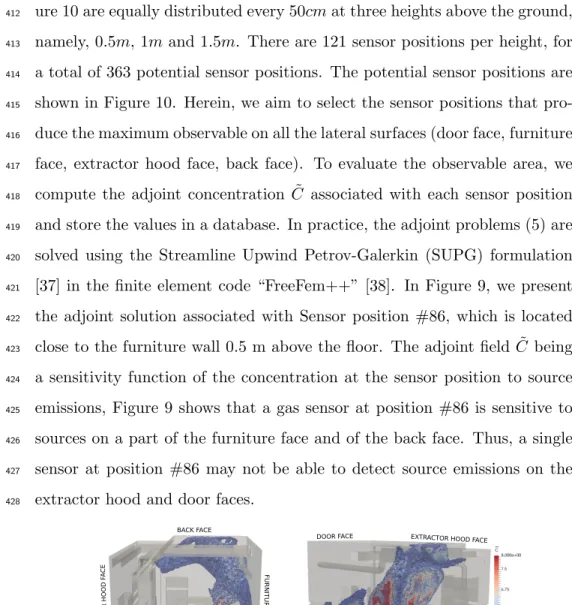
[37] in the finite element code “FreeFem++” [38]. In Figure 9, we present
421
the adjoint solution associated with Sensor position #86, which is located
422
close to the furniture wall 0.5 m above the floor. The adjoint field ˜C being
423
a sensitivity function of the concentration at the sensor position to source
424
emissions, Figure 9 shows that a gas sensor at position #86 is sensitive to
425
sources on a part of the furniture face and of the back face. Thus, a single
426
sensor at position #86 may not be able to detect source emissions on the
427
extractor hood and door faces.
428 DOOR FACE EX TR A CTOR HOOD F A CE FURNIT URE F A CE BACK FACE BACK FACE DOOR FACE FURNIT URE F ACE
EXTRACTOR HOOD FACE
~
Figure 9: Simulation of the adjoint concentration ˜C associated with the optimal sensor
position #86
To quantify the observable on each lateral face, we use the observable
criterion (8), taking into account the sensor features. Herein, we consider
430
that the source emission to be detected has an amplitude of approximately
431
10ppm on a surface of approximately 0.25m2 and that the limit of detection
432
of the sensor is 0.01ppm, i.e. As= 0.25m2, S = 10ppm and dIm= 0.01ppm
433
in Eq. (8). The observable criterion (8) involving the ratio AsS/dIm, the
ob-434
servability results presented in the next paragraphs will be the same for other
435
combinations of As, S and dIm, as long as AsS/dIm= 250. For each
poten-436
tial sensor position, we compute the observable criterion and determine the
437
observability on the four lateral walls. The highest observable area, which
438
is approximately 7m2, is obtained for Sensor position #86. Consequently,
439
Sensor #86 is considered to be the optimal placement of the first sensor.
440
In Figure 10, we use sectors to represent the sensor positions with
“‘accept-441
able observability”, i.e. more than half of the maximum 7m2 observability.
442
Note that 15% (64 positions) of all the potential sensor positions satisfy this
443
criterion. These results highlight the fact that haphazard placement of gas
444
sensors may make it impossible to detect source emissions.
445
Figure 10 shows that most of the sensors are sensitive to source emissions on
446
the furniture and back faces. Only 6 sensor positions (resp. 8 sensor
posi-447
tions) can cover a part of the extractor hood face (resp. the door face). We
448
can see that the observable areas differ depending on the height of the sensor
449
because the air flow is highly three-dimensional in an indoor environment.
450
After fixing Sensor #86 as the first optimal sensor position, the proposed
451
numerical strategy selects Sensors #9, #235 and #268 as the optimal
po-452
sitions of four sensors to maximize the observable area on the wall faces.
453
The optimal positions are represented by red circles in Figure 10, and the
454
associated observability maps are shown in Figure 11. Sensors #86 and #9
455
are selected to cover both the furniture face and the back face.
less, Sensor #86 is sensitive to source emissions on the upper part of the
457
furniture face, whereas Sensor #9 can detect sources on the lower part. The
458
sensitivity of the gas concentration at Sensor position #9 to sources
emit-459
ted from the lower part between the furniture and the wall is due to the air
460
flow. Indeed, the air flow from the second ventilation grid passes under the
461
furniture and licks the lower part of the furniture wall (see Figure 8). Then,
462
the main part of the flow goes out from the corner of the furniture and the
463
door faces, where Sensor #9 is located. Sensor #235 provides information
464
for the extractor hood face and covers additional areas on the back face.
465
Finally, the observability on the door face is provided by the fourth sensor,
466
that is, Sensor #268.
467
Let us consider Sensor positions #86, #9, #235 and #268 and study the
468
influence of the LOD on the observability of the sources. The parameters As
469
and S are kept at 0.25m2 and 10ppm. In Figure 11, we show the observable
470
area associated with each sensor for a 10 ppb LOD and for a 2 ppb LOD.
471
As expected, a lower sensor LOD increases the observable area. At a 10
472
ppb LOD, Sensor #86 can detect sources on a portion of the furniture and
473
back faces. When the LOD is decreased to 2 ppb, sources can be detected
474
on a larger surface of the furniture and back faces and on the door and
475
extractor hood faces, which were not observable at a 10 ppb LOD. Similar
476
results are obtained for Sensor #235. Reducing the LOD to 2 ppb enables
477
the observation of new surfaces, such as the door face. Nevertheless, we can
478
see an exception for Sensor #9. In this case, as the flow is confined between
479
the wall and the furniture, the observable area is slightly increased for a
480
2 ppb LOD compared to that for a 10 ppb LOD. Finally, we observe that
481
some wall areas are covered by multiple sensors when the LOD is 2 ppb.
482
In the last paragraph, we propose numerical validation of the observable
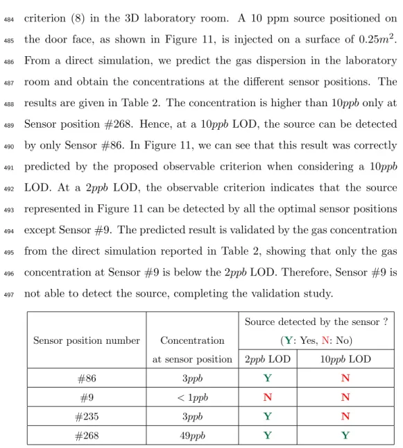
criterion (8) in the 3D laboratory room. A 10 ppm source positioned on
484
the door face, as shown in Figure 11, is injected on a surface of 0.25m2.
485
From a direct simulation, we predict the gas dispersion in the laboratory
486
room and obtain the concentrations at the different sensor positions. The
487
results are given in Table 2. The concentration is higher than 10ppb only at
488
Sensor position #268. Hence, at a 10ppb LOD, the source can be detected
489
by only Sensor #86. In Figure 11, we can see that this result was correctly
490
predicted by the proposed observable criterion when considering a 10ppb
491
LOD. At a 2ppb LOD, the observable criterion indicates that the source
492
represented in Figure 11 can be detected by all the optimal sensor positions
493
except Sensor #9. The predicted result is validated by the gas concentration
494
from the direct simulation reported in Table 2, showing that only the gas
495
concentration at Sensor #9 is below the 2ppb LOD. Therefore, Sensor #9 is
496
not able to detect the source, completing the validation study.
497
Source detected by the sensor ?
Sensor position number Concentration (Y: Yes,N: No)
at sensor position 2ppb LOD 10ppb LOD
#86 3ppb Y N
#9 < 1ppb N N
#235 3ppb Y N
#268 49ppb Y Y
Table 2: Numerical validation of the adjoint-based observable criterion in the 3D labora-tory room - Concentration at sensor positions #86, #9, #235 and #268 simulated for the source location defined in Figure 11 and verification of the source detection for 2ppb LOD sensors and 10ppb LOD sensors
4. Conclusions & Prospects
498
We proposed a CFD-based virtual testing strategy for the optimal
place-499
ment of gas sensors to efficiently localize surface source emissions in indoor
500
air quality assessment. This strategy relies on a criterion that integrates the
501
adjoint framework and sensor features, such as the limit of detection, to
eval-502
uate, at a reasonable computation cost, the coverage area associated with
503
different sensor positions. We considered the “optimal sensor placement”
504
to be the combination of sensors that maximizes the coverage area. In the
505
two studied applications, we showed that many potential sensor positions
506
observe almost nothing and thus are unable to localize sources, which
high-507
lights the importance of using such sensor placement strategies. Then, we
508
emphasized that the coverage area can be increased not only by adding
sen-509
sors but also by using sensors with a lower limit of detection. Hence, when
510
positioning indoor air quality devices, we have to consider both the limit
511
of detection and the number of sensors. Finally, this work can be extended
512
to the localization of sources emitted inside a defined volume, especially for
513
outdoor air quality purposes.
514
Acknowledgments
515
This work was supported by the FUI 18 MIMESYS funded by
Re-516
gion Ile-de-France, which involves several partners: EcologicSense, TERA,
517
ETHERA, FLUIDYN, CSTB, ESIEE Paris, and IFSTTAR. We also want to
518
thank our colleagues Erick Merliot for the realization of the numerical
mock-519
up of the studied room and Rachida Chakir for the fruitful discussions about
520
the direct simulations of the air flow and gas dispersion.
References
522
[1] T. Hoang, R. Castorina, F. Gaspar, R. Maddalena, P. Jenkins,
523
Q. Zhang, T. McKone, E. Benfenati, A. Shi, A. Bradman, Voc
ex-524
posures in california early childhood education environments, Indoor
525
Air 27 (3) (2017) 609–621.
526
[2] C. Godwin, S. Batterman, Indoor air quality in michigan schools,
In-527
door Air 17 (2) (2006) 109–121.
528
[3] N. Goodman, A. Wheeler, P. Paevere, P. Selleck, M. Cheng, A.
Steine-529
mann, Indoor volatile organic compounds at an australian university,
530
Build. and Environ. 135 (2018) 344 – 351.
531
[4] D. Campagnolo, D. E. Saraga, A. Cattaneo, A. Spinazz, C. Mandin,
532
R. Mabilia, E. Perreca, I. Sakellaris, N. Canha, V. G. Mihucz, T. Szigeti,
533
G. Ventura, J. Madureira, E. de Oliveira Fernandes, Y. de Kluizenaar,
534
E. Cornelissen, O. Hnninen, P. Carrer, P. Wolkoff, D. M. Cavallo, J. G.
535
Bartzis, Vocs and aldehydes source identification in european office
536
buildings - the officair study, Build. and Environ. 115 (2017) 18 – 24.
537
[5] A. Bari, W. Kindzierski, A. Wheeler, M.-E. H´eroux, L. Wallace, Source
538
apportionment of indoor and outdoor volatile organic compounds at
539
homes in edmonton, canada, Build. and Environ. 90 (2015) 114 – 124.
540
[6] Indoor air quality (iaq), pollutants, their sources and concentration
541
levels, Build. and Environ. 27 (3) (1992) 339 – 356.
542
[7] W. H. Organization, Selected pollutants, Tech. rep., WHO Regional
543
Office for Europe (2010).
[8] L. Morawska, P. K. Thai, X. Liu, A. Asumadu-Sakyi, G. Ayoko,
545
A. Bartonova, A. Bedini, F. Chai, B. Christensen, M. Dunbabin, J. Gao,
546
G. S. Hagler, R. Jayaratne, P. Kumar, A. K. Lau, P. K. Louie, M.
Maza-547
heri, Z. Ning, N. Motta, B. Mullins, M. M. Rahman, Z. Ristovski,
548
M. Shafiei, D. Tjondronegoro, D. Westerdahl, R. Williams,
Applica-549
tions of low-cost sensing technologies for air quality monitoring and
ex-550
posure assessment: How far have they gone?, Environ. Int. 116 (2018)
551
286 – 299.
552
[9] D. Bourdin, P. Mocho, V. Desauziers, H. Plaisance, Formaldehyde
emis-553
sion behavior of building materials: On-site measurements and
model-554
ing approach to predict indoor air pollution, J. of Hazard. Mater. 280
555
(2014) 164 – 173.
556
[10] C. Dimitroulopoulou, M. Ashmore, M. Hill, M. Byrne, R. Kinnersley,
557
Indair: A probabilistic model of indoor air pollution in uk homes,
At-558
mos. Environ. 40 (33) (2006) 6362 – 6379.
559
[11] F. Haghighat, P. Fazio, T. Unny, A predictive stochastic model for
560
indoor air quality, Build. and Environ. 23 (3) (1988) 195 – 201.
561
[12] W. Nazaroff, C. G., Mathematical modeling of chemically reactive
pol-562
lutants in indoor air, Environ. Sci. & Technol. 20 (9) (1986) 924 – 934.
563
[13] W. Yan, Y. Zhang, Y. Sun, D. Li, Experimental and cfd study of
un-564
steady airborne pollutant transport within an aircraft cabin mock-up,
565
Build. and Environ. 44 (1) (2009) 34 – 43.
566
[14] G. Gan, H. B. Awbi, Numerical simulation of the indoor environment,
567
Build. and Environ. 29 (4) (1994) 449 – 459.
[15] X. Liu, Z. Zhai, Inverse modeling methods for indoor airborne pollutant
569
tracking: literature review and fundamentals, Indoor Air 17 (6) (2007)
570
419–438.
571
[16] X. Liu, Z. Zhai, Protecting a whole building from critical indoor
con-572
tamination with optimal sensor network design and source identification
573
methods, Build. and Environ. 44 (11) (2009) 2276 – 2283.
574
[17] A. D. Fontanini, U. Vaidya, B. Ganapathysubramanian, A methodology
575
for optimal placement of sensors in enclosed environments: A dynamical
576
systems approach, Build. and Environ. 100 (2016) 145 – 161.
577
[18] D. Papadimitriou, K. Giannakoglou, Computation of the hessian matrix
578
in aerodynamic inverse design using continuous adjoint formulations,
579
Comput. & Fluids 37 (8) (2008) 1029 – 1039.
580
[19] J. Waeytens, P. Chatellier, F. Bourquin, Inverse computational fluid
581
dynamics: influence of discretisation and model errors on flows in water
582
network including junctions, ASME J. Fluids Eng. 137 (9) (2015) 17p.
583
[20] H. Elbern, H. Schmidt, O. Talagrand, A. Ebel, 4d-variational data
as-584
similation with an adjoint air quality model for emission analysis, J. of
585
Environ. Model. and Soft. 15 (2000) 539–548.
586
[21] J. Waeytens, P. Chatellier, F. Bourquin, Sensitivity of inverse
587
advection-diffusion-reaction to sensor and control: a low computational
588
cost tool, Comput. and Math. with Appl. 6 (66) (2013) 1082–1103.
589
[22] J. Waeytens, P. Chatellier, F. Bourquin, Impacts of discretisation
er-590
ror, flow modeling error and measurement noise on inverse
diffusion-reaction in a t-junction, ASME J. Fluids Eng. 139 (5) (2017)
592
10p.
593
[23] J. Sykes, J. Wilson, R. Andrews, Sensitivity analysis for steady state
594
groundwater flow using adjoint operators, Water Resour. Res. 3 (1985)
595
359–371.
596
[24] F. Kauker, T. Kaminski, M. Karcher, M. Dowdall, J. Brown, A.
Hos-597
seini, P. Strand, Model analysis of worst place scenarios for nuclear
598
accidents in the northern marine environment, J. of Environ. Model.
599
and Soft. 77 (2016) 13–18.
600
[25] R. Becker, R. Rannacher, An optimal control approach to a posteriori
601
error estimation in finite elements methods, Acta Numerica, Cambridge
602
Press 10 (2001) 1–102.
603
[26] J. T. Oden, S. Prudhomme, Estimation of modeling error in
computa-604
tional mechanics, J. Comput. Phys. 182 (2002) 496–515.
605
[27] J. Waeytens, L. Chamoin, P. Ladev`eze, Guaranteed error bounds on
606
pointwise quantities of interest for transient viscodynamics problems,
607
Comput. Mech. 49 (3) (2012) 291–307.
608
[28] V. Desauziers, D. Bourdin, P. Mocho, H. Plaisance, Innovative tools
609
and modeling methodology for impact prediction and assessment of the
610
contribution of materials on indoor air quality, Herit. Sci. 3 (1) (2015)
611
28.
612
[29] C. Wang, X. Yang, J. Guan, Z. Li, K. Gao, Source apportionment of
613
volatile organic compounds (vocs) in aircraft cabins, Build. and
Envi-614
ron. 81 (2014) 1 – 6.
[30] B. Clarisse, A. Laurent, N. Seta, Y. L. Moullec, A. E. Hasnaoui, I.
Mo-616
mas, Indoor aldehydes: measurement of contamination levels and
iden-617
tification of their determinants in paris dwellings, Environ. Res. 92 (3)
618
(2003) 245 – 253.
619
[31] V. Akcelik, G. Biros, O. Ghattas, K. R. Long, B. van Bloemen
Waan-620
ders, A variational finite element method for source inversion for
con-621
vectivediffusive transport, Finite Elem. in Anal. and Des. 39 (8) (2003)
622
683 – 705.
623
[32] K. Gurney, R. Law, A. Denning, P. Rayner, D. Baker, P. Bousquet,
624
L. Bruhwiler, Y. Chen, P. Ciais, S. Fan, I. Fung, M. Gloor, M. Heimann,
625
K. Higuchi, J. John, T. Maki, S. Maksyutov, K. Masarie, P. Peylin,
626
M. Prather, B. Pak, J. Randerson, J. Sarmiento, S. Taguchi, T.
Taka-627
hashi, C. Yuen, Towards robust regional estimates of CO2 sources and
628
sinks using atmospheric transport models, Nature 415 (6872) (2002)
629
626–630.
630
[33] X. Liu, Z. Zhai, Location identification for indoor instantaneous point
631
contaminant source by probability-based inverse Computational Fluid
632
Dynamics modeling, Indoor Air 18 (1) (2008) 2–11.
633
[34] W. Liang, X. Yang, Indoor formaldehyde in real buildings: Emission
634
source identification, overall emission rate estimation, concentration
in-635
crease and decay patterns, Build. and Environ. 69 (2013) 114 – 120.
636
[35] A.-L. Pasanen, A. Korpi, J.-P. Kasanen, P. Pasanen, Critical aspects
637
on the significance of microbial volatile metabolites as indoor air
pol-638
lutants, Environ. Int. 24 (7) (1998) 703 – 712.
[36] F. Archambeau, N. M´echitoua, M. Sakiz, Code Saturne: A Finite
Vol-640
ume Code for the computation of turbulent incompressible flows -
In-641
dustrial Applications, Int. J. on Finite Vol. 1 (1).
642
[37] T. J. Hughes, M. Mallet, M. Akira, A new finite element formulation
643
for computational fluid dynamics: Ii. beyond supg, Comput. Meth. in
644
Appl. Mech. and Eng. 54 (3) (1986) 341 – 355.
645
[38] F. Hecht, New development in freefem++, J. Numer. Math. 20 (3-4)
646
(2012) 251–265.
Figure 10: Potential positions of gas sensors at three levels h = 0.5m, h = 1m and h = 1.5m and observability representation by wall surface for sensors with an observable area more than half of the highest observability achieved by Sensor #86 - Optimal sensor
Sensor #86 Sensor #9 Sensor #235 Sensor #268
Observable area for 10 ppb LOD (6.9m2)
Observable area for 2 ppb LOD (31.2m2)
DOOR F ACE FURNITU REFACE BACK F ACE EXTR ACTOR HOOD F ACE EXTRACTOR HOOD F ACE EXTR ACTOR HOOD F ACE EXTR ACTOR HOOD F ACE BACK F ACE BACK FACE BACK FACE FURNITU RE FACE FURNITU RE FACE FURNITU RE FACE DOOR F ACE DOOR F ACE DOOR F ACE
Observable area for 10 ppb LOD (5.4m2)
Observable area for 2 ppb LOD (8.8m2)
Observable area for 10 ppb LOD (5.2m2)
Observable area for 2 ppb LOD (20.8m2)
Observable area for 10 ppb LOD (4.4m2)
Observable area for 2 ppb LOD (21.6m2)
Figure 11: Map of the observable areas associated with gas sensors #86, #9, #235 and #268 at two different LODs (10 ppb and 2 ppb). The total observable areas are indicated in parentheses - Definition of a 0.5m × 0.5m source (white square) for the numerical validation of the observability criterion