ANN BASED APPROACH TO SOLVE GROUNDWATER POLLUTION INVERSE PROBLEM

(1)

HAL Id: hal-00728679

https://hal.archives-ouvertes.fr/hal-00728679

Submitted on 30 Aug 2012

HAL is a multi-disciplinary open access archive for the deposit and dissemination of sci-entific research documents, whether they are pub-lished or not. The documents may come from teaching and research institutions in France or abroad, or from public or private research centers.

L’archive ouverte pluridisciplinaire HAL, est destinée au dépôt et à la diffusion de documents scientifiques de niveau recherche, publiés ou non, émanant des établissements d’enseignement et de recherche français ou étrangers, des laboratoires publics ou privés.

ANN BASED APPROACH TO SOLVE

GROUNDWATER POLLUTION INVERSE PROBLEM

Maria Laura Foddis, Augusto Montisci, Gabriele Uras, Philippe Ackerer

To cite this version:

Maria Laura Foddis, Augusto Montisci, Gabriele Uras, Philippe Ackerer. ANN BASED APPROACH TO SOLVE GROUNDWATER POLLUTION INVERSE PROBLEM. 9th International Conference on Modeling, Optimization & SIMulation, Jun 2012, Bordeaux, France. �hal-00728679�

(2)

“Performance, interoperability and safety for sustainable development”

ANN BASED APPROACH TO SOLVE GROUNDWATER POLLUTION

INVERSE PROBLEM

M.L. FODDIS , A. MONTISCI, G. URAS

DIT / DIEE University of Cagliari 3, via Marengo

09123 Cagliari - Italy

[email protected], [email protected] [email protected]

P. ACKERER

LHyGeS / University of Strasbourg 1, rue Blessig

67084 StrasbourgCedexFrance [email protected]

ABSTRACT: This paper investigates the feasibility of solving the groundwater pollution inverse problem by using

Artificial Neural Networks (ANNs). Different ANNs have been trained to solve the direct problem of associating the characteristics of a source of pollutant to the concentration measured in a set of monitoring wells. In order to solve the inverse problem and to identify the unknown pollution source and their characteristics, the trained ANN is inverted. By fixing the output pattern of the ANN, the proposed procedure is able to reconstruct the corresponding input. The approach has been applied to a real case which deals with the contamination of the Rhine aquifer by carbon tetrachloride (CCl4) due to a tanker accident. This case is well adapted to the problem since numerous concentrations

have been measured at different piezometers and at different time. The location of the source and the beginning of the contamination are known. The ANNs are used to identify the contamination source and the results are compared with the solution obtained with a different approach.

KEYWORDS: artificial neural networks inversion; inverse problems; groundwater modeling; groundwater pollution

source identification.

1 INTRODUCTION

Only a small percentage of water present on Earth is use-ful for human use and 98% of this water is represented by water reserves contained in aquifers. Therefore groundwater represents an important resource for the production of drinking water. However, groundwater is exposed to man-made pollution. One of the major issues for groundwater specialists is the effective management of the groundwater quality because contamination of groundwater may prevent its use for drinking as well as for other domestic, industrial and agricultural purposes. Due to large pollution phenomena, groundwater has be-come increasingly vulnerable and its sustainable man-agement is nowadays extremely important to protect global health. Concerning groundwater resources con-taminations, it should be underlined that in some cases, pollution may result from contaminations whose origins are generated in different times and places from where these contaminations have been actually detected. To address such pollution cases, it is necessary to develop specific techniques that allow to identify in time and space the behaviour of unknown contaminant sources. In general, the identification and delineation of the source of a contaminant plume is of utmost importance regard-ing both the improvement of management policies and

the planning of subsurface remediation in the polluted site.

In this work, the Artificial Neural Networks (ANNs) have been used for defining an innovative ANNs based methodology for the identification of unknown contami-nant sources and their characteristics. In particular, start-ing from the effect caused by a specific phenomenon, we attempt to determine the cause that generated such phe-nomenon by resolving of the so-called inverse problem. Various studies dealing with the resolution of inverse problems in groundwater contaminations have been re-cently carried out by several authors, however works us-ing the ANN approach are less popular. Fanni A. et al (2002) proposed the use of the neural network to capture the functional relationship between geometrical and chemical properties of the contaminants and the hydro-logical map of the basin in prefixed measurement points. Iqbal Z. and Guangbai C. (2003) proposed an inverse modeling approach, using artificial intelligence for the identification of non-point source pollution based on pol-lution indicators in storm water and agriculture runoff. Mahar P.S. and Datta (2000) proposed a methodology based on nonlinear optimization model for estimating unknown magnitude, location and duration of groundwa-ter pollution sources by using measured values of pollut-ant concentration at selected locations. Singh and Datta (2007) proposed an ANN based methodology to identify unknown groundwater pollution sources, when a portion

(3)

MOSIM’12 - June 06-08, 2012 - Bordeaux - France

of the concentration observation data is missed. Tapesh K Ajmera and A. K. Rastogi (2008) applied three mod-els, each based on artificial neural networks, for predic-tion of zonal groundwater transmissivity. Zio E.(1997) investigated the feasibility of solving the inverse prob-lem by using artificial neural networks. He considered a simple analytic model of contaminant transport due to a point source in stationary flow field to generate simu-lated concentration histories for various values of the dispersion coefficient. The simulated observations have been used to train the ANN to identify the value of the associated dispersion coefficient.

The originality of the methodology proposed in the this paper lies in the approach used to solve the inverse prob-lem, which consists of inverting the neural model instead of solving the equations that described the physical sys-tem.

In particular, different ANNs were trained to solve the direct problem with the objective of associating the input patterns (which represent the pollution source character-istics) with the output patterns (which represent the measures acquired in the monitoring wells). To solve the inverse problem and to identify the unknown pollution source characteristics, the trained ANN has been in-verted. By fixing the output pattern of the ANN, the pro-posed procedure is able to reconstruct the corresponding input.

The approach is used to identify contaminant point sources (locations and fluxes over time) for groundwater quality problems. The procedure has been validated on a real case which deals with the contamination of the Rhine aquifer by carbon tetrachloride (CCl4) due to an

accident occurred in 1970 (Benfeld – France). This case is well adapted to the problem since numerous concen-trations have been measured at different piezometers and at different time. Moreover the location of the source and the beginning of the contamination are known. The pol-lution source behaviour at the accident location and the exact amount of the chemical infiltrated are unknown and these constitute the main issue for its individuation and remediation. Therefore, the objective is to recon-struct the temporal variations, injection rates and dura-tion of the activity of the unknown contaminant source. The methodology has been used to solve the inverse problem for identifying the contamination source based on measurements of the contamination concentration curves in monitoring wells. An ANN is trained to solve the direct problem of associating input patterns, which represent the pollution source, with the output patterns, which represent the measures acquired in the wells. To solve the inverse problem and to identify the unknown pollution source behaviour, the trained ANN is inverted, by fixing the output pattern and finding the correspond-ing input. The results are compared with the known solu-tion.

2 2 MATERIALS AND METHODS

2.1 Multi Layer Perceptron (MLP) network model

Multi Layer Perceptron (MLP) ANNs are used to model the system under study. Such neural model is trained by using a set of patterns created by means of a flux and transport contaminant modelling software, where the pat-terns describe both the source of contaminant and the set of measurements in the monitoring wells, which repre-sents the input and the output of the network respec-tively. input output

x

u

1

W

₂ 1

b

₂

y

h

. .

. . .

input output

x

u

1

W

₂ 1

b

₂

y

h

. .

. . .

Figure 1 : MLP structure

The ANN is trained by using the standard Levenberg-Marquard algorithm.

The trained ANN realizes a relationship between input and output patterns described by the following algebraic equations system:             u b h W y h y b x W 2 2 1 1 ) ( layer Output layer Hidden layer Input  (1) Where:

x

is the input of the network,

1

W

is the weights matrix of the input layer,

1

b

is the bias vector of the input layer,

y

is the input of the hidden layer,

h

is the output of the hidden layer,

)

(



is the hidden neurons logistic activation function,

u

is the output of the network,

2

W

is the weights matrix of the output layer,

2

b

is the bias vector of the output layer.

Determining the characteristics of the pollutant source, implies solving an inverse problem.

As described in Carcangiu S. et al. (2008), if in the in-verse problem, the relationship between the design pa-rameters and objective functions is not bi-univocal, it is not possible to solve the inverse problem as a direct problem.

(4)

For this reason, in this work, the problem is modelled as a direct problem and the inversion is performed by in-verting the trained ANN, by solving system eq. (1) for the input

x

given an assigned value of the output

u

. In section 2.3, the inversion method is enlightened.

2.2 ANN pattern feature extraction techniques

Data which usually describe groundwater flow and con-taminant transport problems are characterized by huge volume and strong redundancy of information, so that in general it is possible to pre-process the data by reducing the volume of data and at the same time without a mean-ingful loss of information.

In the proposed approach the feature extraction tech-niques are carefully chosen in compliance with two im-portant requirements: having a high rate of compression and saving the information which guarantees to obtain a significant correspondence between the back trans-formed data and the original values.

The feature extraction adopted in this work is structured as follows. First the two-dimensional discrete fast Fou-rier transform (2D-FFT) is calculated for both the input and output matrices. Secondly the frequency components that are below a stated threshold of energy content are eliminated. Finally a further reduction is performed by means of the Principal Component Analysis (PCA) method.

For the first step, each matrix (groundwater flow and transport numerical simulation example model) is trans-formed from space-time domain into frequency domain representation by applying the 2D-FFT. The matrices in the frequency domain are characterized by replicas of the same information, so only one replica for each matrix is considered. The values related to input and output matri-ces are stacked into a unique column, to constitute the pair input-output for a specific case. Vectors correspond-ing to the traincorrespond-ing examples have been joined to form a global matrix, so that the two patterns of input and out-put matrices are reorganized to form two global matri-ces: one for the input patterns concerning of the sources features in frequency domain and one for the output pat-terns regarding the wells features in frequency domain. For the second step, the matrices frequency components of each matrix have been compared on the basis of their amplitude. Separately, for input and output matrices, a threshold has been set in order to select only the most significant frequency components. The remaining com-ponents and the corresponding phases comcom-ponents have been set to zero. The value of the threshold is determined by seeking a crossover between the information loss and the size of matrices. In order to successively apply the PCAs, the matrices have to have a number of rows less or equal to the number of columns, namely, the number of examples has to be higher than the number of features For the third step, the normalization (range [-1,+1]) and PCA were applied. Before applying the PCA, the matrix needs to be normalized so that each row has zero means and standard deviations equal to 1. By means of PCA, systematic information initially dispersed over a large

matrix of variable input (often interrelated) is extracted and condensed in a few abstract variables.

2.3 Inversion procedure description

As previously mentioned, once the training of the ANN is terminated, the trained network is inverted for solving the inverse problem, namely, on the basis of the output of the ANN the corresponding input is calculated by ex-ploiting the method described in Carcangiu S.et

al.(2007) and in Fanni A. and Montisci A.(2003).

As in any identification problem, it is fundamental that the uniqueness of the solution is guaranteed. This im-plies that the two linear equations systems in (1) are de-termined or over-dede-termined, then the number of input neurons has to be greater or equal to the number of hid-den neurons and this has to be higher or equal to the number of output neurons. Secondly, for the same rea-son, the first and the second connections weights matri-ces

1

W

and

2

W

have to be full-rank. Such a constraint could give rise to some trouble. In general the learning algorithms are not able to monitor and control the rank of connecting matrices during the training phase, so that a trial and error approach has to be adopted. The parame-ter that can affect such features of the ANN is, generally speaking, the approximation degree of the representation of both input and output data: this means that increasing the precision used to describe the input and output data in general does not give rise automatically to fully ranked matrices. From this point of view, the trial and error procedure should consist in seeking the best ap-proximation level which guarantees the invertibility of the ANN.

To invert the ANN we need to solve equations system (1) for an assigned output pattern

u

. If the constraints

on the rank of

1

W

and

2

W

are fulfilled, solving the sys-tem (1) is quite simple, as the three unknown patterns

h

,

y

and

x

can be determined one after the other univo-cally. In the first step we exploit the linear relation with the known output

u

for finding the pattern

h

. If the number of hidden neurons is greater than that of output ones, we can obtain the mean squared error solution by pre-multiplying the system by the transposed of the coef-ficient matrix:





2



2 1 2 2

W

u

b

W

h



T







T







(2) In the second step the vector y is determined. The second equation in (1) states a biunivocal relation between y and

h, so that the vector y can be calculated as:

 

h

y





1 (3) In the third step the input pattern x is determined. In this case we can repeat the same reasoning adopted in the first step, so that we can write:





1



1



1 1 1

W

y

b

W

x



T







T





(4)

(5)

This step concludes the ANN inversion procedure. In order to obtain the real profile of the contaminant source, the pattern x has to be back transformed, by in-verting the feature extraction procedure.

Remark. Equations (2) and (4) related to the first

and third step respectively, refers to the general case of over-determined system, then the number of rows of the coefficient matrix is greater than the number of columns. The fact that these equations systems are over-determined could seem in contrast with the fact that a solution must be achieved. Actually, the approximation error of the ANN cannot be completely eliminated, so that a number of equations greater than the exact mini-mal number could aid to improve the quality of the esti-mate. It is worth to note that, if the coefficient matrix is squared, namely if the number of neurons in the two connected layers is the same, we do not need to left mul-tiply the equation by the transpose of the coefficient ma-trix.

3 RESULTS AND DISCUSSION

The performance of the proposed methodology has been evaluated by applying it to the case of Alsatian aquifer pollution, where the characteristics of the pollutant source have to be determined.

3.1 General description of the Alsatian aquifer

Alsatian aquifer is located in the southern part of the Upper Rhine valley. The Upper Rhine Graben is a seg-ment of the European Cenozoic rift system that devel-oped in the north-western forelands of the Alps. It is ex-tended over 300 km, from Basel (Switzerland) in the south to Frankfurt (Germany) in the north, with an aver-age width of approximately 40 km. It is flanked, in the south, by the Vosges and Black Forest (Schwarzwald) mountains, to the west and the east, respectively (Ber-trand G.et al., 2006), see Figure 1.

The Alsatian aquifer surface is over 3000 km2_and

con-tains a volume of alluvial about 250 billion m3. It repre-sents one of the largest fresh water reserves in Europe(Vigouroux, P.et al.,1983). The groundwater res-ervoir contains about 50 billion m3_{of water, with an}

an-nual renewal of 1.3 billion m3_.

This large aquifer has a vital importance since it supplies to the 75% of the drinking water requirements, the 50% of the industrial water needs and the 90% of the irriga-tion water needs in Alsace. The Alsatian part of the Rhine aquifer has a surface length of 160 km and a maximum width of 20 km (Bertrand G.et al., 2006), (Hamond, M. C., 1995).

The groundwater reservoir is part of a complex hydro-system, which includes frequent exchanges between the rivers and the aquifer which vary with the seasons, and are caused by the proximity between the surface and the groundwater. This aquifer is highly exposed to contami-nation from rivers (Stengera A. and Willingerb M., 1998).

Figure 2 : The Rhine Valley and the geographic situation of the Alsatian aquifer

Alsatian aquifer is an extensive alluvial aquifer with a layered structure composed by a random superposition of different alluviums (clay, sand fine to rough, gravels, coarse…). This permeable alluvial has a thickness of a few meters at the Vosgean edge, and 150 m to 200 m in the centre of the Rhine plain (Hamond, M. C., 1995).

3.2 History of the pollution by CCl4 in the aquifer

Alsace is a region where groundwater has a very impor-tant role in water supply. On the other side, it is a heavily industrialised area, so the quality of groundwater is jeop-ardized by industrial contamination. This sort of pollu-tion is harmful for drinking water.

In 1970 a tanker truck containing CCl4 property of a

Dutch company, capsized in the north of Benfeld (a small town located about 35 km south of Strasbourg, eastern France). In spite of the efforts of the firemen to control the spilling of the chemical, an important quan-tity of it could not be recovered. According to a note of SGAL (Service Géologiqued’Alsace-Lorraine) of De-cember 21th 1971 about 4000 litres of CCl4 were spread

in the area of the accident, infiltrating into the ground or disappearing by evaporation (Hamond, M. C., 1995). In 1991, the analyses carried out by BRGM (Bureau de Re-cherche Géologique et Minière) showed abnormal quan-tities of CCl4 in the supplies of drinking water located

(6)

exceeded the safe limits recommended by the World Health Organization (2 μg/l). This high level of CCl4

concentration has caused a serious problem in the region by contaminating the most important drinking water source in the area (Aswed T., 2008).

3.3 ANN to study the Alsatian aquifer

In order to train, validate and test the ANN a data set of patterns has been constructed through a coherent number of hydrogeological scenarios, based on an 3D model of the domain developed by Taef Aswed in 2008 (Aswed T., 2008).

In a first time, the ANN was trained to solve the direct problem. In this part of the application, the network was trained by means of examples, to associate the pollution sources features with the corresponding output contami-nant concentration at monitoring wells. The input pat-terns were made of the pollution source features in terms of the injection rates in four underground layers. The output patterns were contaminant concentration observa-tion data at 45 monitoring wells. Sources and monitoring wells are related by a biunivocal relationship. It means that to each contaminant concentration behaviour in monitoring wells corresponds only one source contami-nant behaviour.

In a second time, the trained network was inverted in or-der to solve the inverse problem. On the basis of the known contaminant concentration data in monitoring wells, the pollution sources injection rates in the cross section have been identified.

3.4 Groundwater flow and contaminant transport numerical model

The CCl4 Alsatian aquifer pollution has been the subject

of several studies that address the hydrodynamic state of the aquifer and the pollution migration (Aswed T., 2008), (Vigouroux P.et al.,1983)(Beyou, L., 1999). The 3D ground water flux and contaminant transport numeri-cal model used for constructing the patterns was numeri- cali-brated using measured data of CCl4 concentration, that

were collected during 12 years (from 1992 to 2004) and simulations were performed from 1970 to 2024.

The patterns have been simulated using the non com-mercial numerical software TRACES (Transport or Ra-dioActiver Elements in the Subsurface), that combines the mixed-hybrid finite element and discontinuous finite element to solve the hydrodynamic state and mass trans-fer in the porous media (Hoteit H. and Ackerer P., 2003). The contaminated zone is enclosed within a 3D domain of 6 km width, 20 km length, and about 110 m depth. This aquifer domain is discretized using a 3D triangular prismatic grid with 25388 nodes and 45460 elements. According the estimated geometry of the cross sections (the landfill site was divided into 8 zones by soil type) the domain is discretized into 10 layers. The contaminant source is locate in the first 4 layers (depth 16, 4, 5 and 5 m from top to bottom). The volume of contaminated aq-uifer is about 230 m3_{to 1300 m}3_{. The surface of}

con-taminant infiltration is about from 7 to 37 m2_{(Aswed T.,}

2008).

Using TRACES, various states of pollution sources have been constructed adjusting the source characteristics in terms of injection rates over the vertical section. 104 ex-amples were constructed with the same duration of activ-ity of about 31 years (11520 days) and were located in the same positions in the domain (accident site in Benfeld - France ). So for each of the 104 sources, a dif-ferent evolution of the contaminant concentration in the time for the 4 layers in the numerical domain has been considered. The total time of simulation is about 54 years (20000 days).

3.5 ANN pattern construction: elaboration and fea-tures extraction

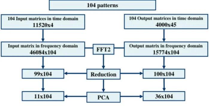
The example patterns obtained with TRACES consist of 208 matrices of contaminant concentrations:

 104 matrices correspondent to the pollution sources features. These have dimension of [11520x4]. 11520 represents the time (days) and 4 represents the layers in the source loca-tion;

 104 matrices correspondent contaminant con-centration in monitoring wells. These have di-mension of [4000x45]. 4000 represents the time (one value each five days) and 45 represents the monitoring wells in the domain.

The 104 input matrices and the 104 output matrices have been reorganized to form two unique big matrices: one for the input and one for the output. The two groups of input and output matrices were considered separately. Several data pre-processing can be used and the choice is strictly linked to the ANN approach selected. When In-put and OutIn-put matrices are too large to be processed through the ANN, data pre-processing may be performed in order to drastically reduce their dimension. The fea-ture extraction techniques, applied in this case, have been chosen on the basis of preliminary neural models trials.

104 Output matrices in time domain

4000x45

104 Input matrices in time domain

11520x4 100x104 99x104 FFT2 PCA Reduction 104 patterns

Input matrix in frequency domain

46084x104

Output matrix in frequency domain

15774x104

36x104 11x104

Figure 3 : matrices reduction schema

For the first step, the 2D-FFT has been calculated for each matrix, using Matlab. From the so obtained fquency matrices, the replicas are removed and the re-maining components are stacked to form a column vec-tor where the first half of the column is constituted by the amplitudes and the second half by the phases. For

(7)

each analyzed case we obtain two vectors: an input vec-tor with [46084] elements and an output vecvec-tor with [15774] elements.

Vectors corresponding to different cases have been joined to form a matrix where each column corresponds to one example. The input matrix has dimension [46084x104],and the output matrix has dimension [15774x104].

In the second step, the frequency components of each matrix have been compared on the basis of their ampli-tude. For both input and output matrices, a threshold has been set in order to select only the most significant 2D-FFT components. The components whose amplitude is below the said threshold and the corresponding phases components have been set to zero. The value of the threshold is determined by seeking a crossover between the approximation of the acquired data and the dimen-sion of the input and output matrices. The number of re-maining values is pushed to have a number of the rows less or equal to the number of the examples, otherwise PCAs cannot be applied. As a result of this second re-duction, the input matrix has dimension [99x104] and the output matrix has dimension of [100x104].

The obtained dimensions of the two matrices allow us to apply the PCA. A value corresponding to the percentage of information loss has to be defined in order to apply the transform. By means of a trial and error procedure, directed to define the minimum number of principal components necessary to allow a good ANN perform-ance, the determined loss value was: 210-3_{for the input}

and 10-7_{for the output. The obtained input matrix has}

dimension [11x104] and the output matrix has dimension [36x104].

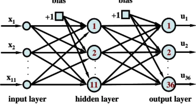
3.6 Multi Layer Perceptron (MLP) network devel-opment and inversion

One 11-11-36 MLP has been implemented and trained with the Levenberg-Marquardt algorithm on the set of 45 input-output pairs. bias bias 1 2 +1 x1 x2 x11 1 2 u1 u2 u36 +1

input layer hidden layer output layer

. . . . . . . . . bias bias 11 36 1 2 +1 x1 x2 x11 1 2 u1 u2 u36 +1

input layer hidden layer output layer

. . . . . . . . . 11 36

Figure 4 : 11-11-36 MLP for the study of the Alsatian aquifer pollution source

The training of the ANN is a critical part of the proposed process. In fact a special attention has to be paid to train the ANN in such a way that it is able to generalize the information contained in the training set. To this end, during the training phase the error is evaluated even in the validation set. When the error starts to increase, the

training is interrupted. Based on the Cross Validation stop criterion the patterns are divided in three sets: 74 in the training set, 19 in the validation set and 11 in the test set.

Once the training phase is completed, the trained net-work is inverted for solving the inverse problem, by as-sociating to the contaminant concentrations measured in the 45 monitoring wells the corresponding contaminant concentrations of the pollution source. This is done by applying the procedure described in section 2.3.

As a preliminary check, the rank of both

1

W

and

2

W

has been calculated and they resulted be full-rank. Therefore, the inversion procedure has been applied, ob-taining the results described in the following section.

Remark 1. In this case, the weights matrices were full

rank. However, if the weights matrices are not full rank it means that the solution of the inversion is not unique. As described in Section 2.3, in general the possibility to have full rank connections matrices depends on the pre-cision one uses to describe the patterns. As a conse-quence, the full rank condition can be accomplished by seeking a crossover between the dimension of the pat-terns and the invertibility of the network.

Remark 2. In the examined case, the inversion

proce-dure furnished at the first step a solution with acceptable precision. This is not always guaranteed, in the sense that the found solution could not produce a configuration of monitoring wells similar to the fixed one. This means that the ANN model is not accurate near the found solu-tion and it needs to be better trained, by adding new ex-amples to the training set, first of all the configuration corresponding to the just found inverse solution. Then, a new simulation with TRACE is performed in order to have the input-output pair which is added to the training set. By iterating such procedure, a rising number of training examples will concentrate around the searched solution, allowing the ANN to improve the accuracy in this region and finally to be successfully inverted.

3.7 Results

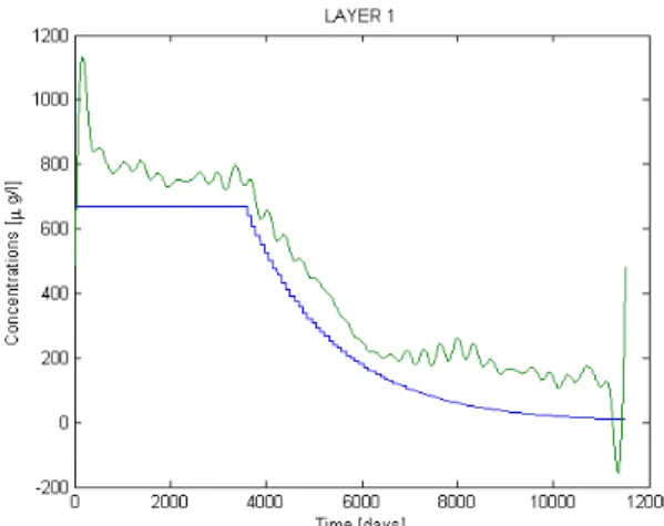
The following figures (Figure 5, 6 ,7 and 8) show the comparison between the pollution source behaviour re-constructed by Aswed (Aswed T., 2008) (blue) and the diagram obtained by inverting the ANN (green) for the 4 layers.

(8)

Figure 5 : Simulated (blue) and the inverted (green) pollution source behavior of the first layer.

Figure 6 : Simulated (blue) and the inverted (green) pollution source behavior of the second layer.

Figure 7 : Simulated (blue) and the inverted (green) pollution source behavior of the third layer.

Figure 8 : Simulated (blue) and the inverted (green) pollution source behavior of the fourth layer. As one can see, the calculated behaviour of the source satisfactorily fits the trend reported in (Aswed T., 2008). The approximation is better in the deepest layers, where the concentration is higher, due to the deposition of the contaminant during the time. The ripple and the peaks does not correspond to a real behaviour of the source but they are due to the large number of frequency compo-nents that have been removed during the data reduction. Standard signal filtering procedures, like Kalman filters, could be applied in order to improve the appearance of the signal, but this would be useless for an expert as-sessment. The boundary peaks are physically not expli-cable and these have to be associated to numerical ef-fects.

4 CONCLUSION

In this paper an ANN-based approach for solving inverse problems in aquifers pollution has been presented. A crucial aspect of the procedure is represented by the training of the ANN, which has to guarantee a satisfac-tory approximation of the physical system, but at the same time it has to fulfil several requirements, for exam-ple in terms of number of neurons, and rank of the con-nections weights matrices. The trained ANN is analyti-cally inverted to solve the inverse problem, which con-sists in determining the profile of the pollutant source on the basis of a set of measures in monitoring wells. This procedure has been tested on a real case: an acci-dent, which took place in the North-East of France in 1970, gave rise to a contamination by carbon tetrachlo-ride in the Alsatian aquifer.

Various numerical model scenarios of the CCl4

contami-nation in Alsatian aquifer have been generated to train the ANN. Complex and heterogeneous hydrogeology systems are extremely difficult to model mathematically. However, it has been proved that ANN’s flexible struc-ture can provide simple and reasonable solutions to vari-ous problems in hydrogeology. The proposed approach appears to be an interesting and relevant tool for this kind of non-linear problem.

(9)

REFERENCES

Aswed T., 2008. PhDthesis: Modélisation de la pollution

de la nappe d’alsace par solvants chlores. Université

Louis Pasteur, Institut de Mécanique des Fluides et des Solides, UMR CNRS 7507, Strasbourg, France, pp 40-42.

Bertrand G.,Elsass P., Wirsing G., Luzc A., 2006.

Quaternary faulting in the Upper Rhine Graben revealed by high-resolution multi-channel reflection seismic.C. R. Geoscience 338, pp. 574-580.

Carcangiu S., Di Barba P., Fanni A., Mognaschi M.E., Montisci A., 2007. Comparison of multi objective

optimisationapproaches for inverse magnetostatic problems. COMPEL: Int. J. for Computation and

Maths in Electrical and Electronic Eng., Vol. 26, Number 2, pp. 293-305.

Fanni A., Uras G., Usai M., Zedda M.K., 2002. Neural

Network for monitoring. Groundwater. Fifth

International Conference on Hidroinformatics, Cardiff, UK, 1-5 July 2002, pp. 687-692.

Fanni A., Montisci A., 2003. A Neural Inverse Problem

Approach for Optimal Design. IEEE Transaction on

Magnetics, Vol. 39, No 3, May 2003, pp. 1305-1308. Hamond, M. C., 1995. Modélisation de l’extension de la

pollution de la nappe phréatique d’Alsace par le tétrachlorure de carbone au droit et à l’aval de Benfeld. Mémoire pour le DESS sciences de

l’environnement. Institut de Mécanique des Fluides et des Solides, Strasbourg, France.

Hoteit H. and Ackerer P., 2003. TRACES user’s guide V

1.00.Institut mécanique des fluides et des solides de

Strasbourg, France.

Iqbal Z. and Guangbai C., 2003. Inverse modelling to

identify nonpoint source pollution using a neural network, Taihu lake watershed, China,

environmental hydrology. The Electronic Journal of

the International Association for Environmental Hydrology, http://www.hydroweb.com.

Mahar P.S. and Datta B., 2000. Identification of

pollution sources in transient groundwater systems.

Water Resources Management vol 14, pp. 209-227. Singh R.M. and Datta B., 2007. Artificial neural network

modelling for identification of unknown pollution sources in groundwater with partially missing concentration observation data. Water

ResourceManagement Volume 21, Number 3, March 2007, pp. 557– 572.

Stengera A. and Willingerb M., 1998. Preservation

value for groundwater quality in a large aquifer: a contingent-valuation study of the Alsatian aquifer.

Journal of Environmental Management, Volume 53, Issue 2, June 1998, pp. 177-193.

AjmeraT. K.and A. K. Rastogi, 2008. Artificial neural

network application on estimation of aquifer transmissivity. Journal of Spatial Hydrology, Vol.8,

No.2, pp.15-31.

Zio E., 1997. Approaching the inverse problem of

parameter estimation in groundwater models by means of artificial neural networks. Progress in

Nuclear Energy, Elsevier Science Ltd, Vol 31, Number 3, pp. 303-315.

Vigouroux P., Vançon J. P. and Drogue C., 1983.Conception d’un model de propagation de

pollution en nappe aquifer-Exemple d’application à la nappe du Rhin. Journal of Hydrology 64, Issues

1-4, pp. 267-279.

Beyou L., 1999.Modélisation de l’impact d’une pollution

accidentelle de la nappe phréatique d’Alsace. Cas du déversement de CCl4 à Benfeld. Projet fin d’études