HAL Id: hal-00758436
https://hal.sorbonne-universite.fr/hal-00758436
Submitted on 6 May 2013
HAL is a multi-disciplinary open access
archive for the deposit and dissemination of
sci-L’archive ouverte pluridisciplinaire HAL, est
destinée au dépôt et à la diffusion de documents
Astrometry and Light Curves of Asteroids with the
SUBARU Telecope
Jean Souchay, Damya Souami, Fumi Yoshida, J. Anderson, Tsuko Nakamura,
Budi Dermawan, N. Yagi, Francois Taris, Nicolas Bures
To cite this version:
Jean Souchay, Damya Souami, Fumi Yoshida, J. Anderson, Tsuko Nakamura, et al.. Astrometry and
Light Curves of Asteroids with the SUBARU Telecope. International Workshop NAROO-GAIA ”A
new reduction of old observations in the Gaia era”, Paris Observatory, Jun 2012, Paris, France. pp.
209-213. �hal-00758436�
J.Souchay(1),D.Souami(1,5),F. Yoshida(2),J.Anderson (3),T.Nakamura(2),B.Dermawan(4), M. Yagi(2),F.Taris(1), N.Bures(1)
(1) SYRTE, UMR8630 du CNRS /UPMC, Observatoire de Paris, 61 Avenue de l’Observatoire, F-75014, Paris; E-mail:”[email protected]”
(2) National Astronomical Observatory of Japan 2-21-1 Osawa, Mitaka, Tokyo 181 (3) Space Telescope Science Institute,3700 San Martin Drive, Baltimore,MD21218,USA (4) Bandung Institute of Technology, Jalan Ganesha 10, Bandung, Indonesia
(5) Universit´e Pierre et Marie Curie (UPMC), 4 place Jussieu, Paris, France
Abstract
We present the reductions of observations of a single ecliptic field, carried out over one night in September 2, 2002, at the focus of the SUBARU 8.2 m telescope. The frames necessary for the reduction were retrieved through the database SMOKA (Subaru Mitaka Okayama Kiso Archive System) High frequency multi shots imaging of the fields enable to detect sub-kilometric asteroids and to perform astrometric and photometric reduction, leading in some cases to the extraction of light curves.
1
Introduction
After developing wide field imaging reduction techniques at the laboratory SYRTE (Paris Observatory), we decided to proceed to a data mining of wide fields images taken at the focus of large telescopes, to test our software on very deep fields. Our choice was made on the SMOKA database (Subaru Mitaka Okayama Kiso Archive system). In particular we were attracted by a series of images performed over two consecutive nights, on September 2 and 3, 2002, that is to say roughly 10 years ago. These images were taken with the Suprime-Cam, which is a 80-mega pixel (10240× 8192) mosaic camera, covering a wide field of 34’× 27’, and is composed of ten 2k × 4k CCD chips, with a resolution of 0”.202 per pixel. The images were taken by F.Yoshida and T. Nakamura in the frame of an observational program called SMBAS (Sub km Main Belt Asteroid Survey).
Two different fields, close to the ecliptic plane, were observed during the two consecutive night sessions mentioned above, called respectively FIELDA and FIELDB. This observational two nights session was called SMBAS-III, as a third campaign following SMBAS-I (February 22 and 25, 2001) and SMBASII (October 21, 2001) The second field was chosen at the east side of the first one, to avoid common objects. Both FIELDA and FIELDB were surveyed with the R band and the B band. The exposure time was set at 120 seconds. This choice comes from the fact that outer edge MBA’s (Main Belt Asteroids) move with an apparent angular rate of roughly 0.5”/mn, whereas the seeing at Mauna Kea has an average value of 0.9”. Therefore a longer exposure time would result in non pointlike objects, not appropriate for detection and measurements.
Data reduction was performed using the SDFRED1 software provided by SMOKA (Yagi et al.,2002; Ouchi et al.,2004) and also using the standard IRAF procedures as it was done previously by two co-authors of this paper (Yoshida et al., 2003; Yoshida et al., 2007). First, chip by chip master flat and bias images are generated, then averaged.
Astrometry and Light Curves of Asteroids
with the SUBARU Telescope
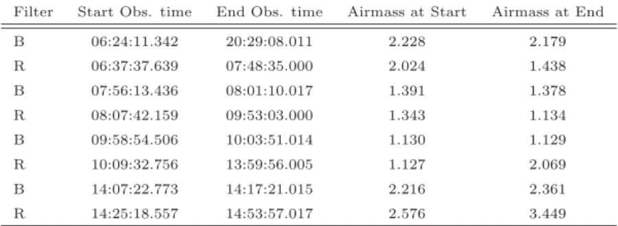
Filter Start Obs. time End Obs. time Airmass at Start Airmass at End B 06:24:11.342 20:29:08.011 2.228 2.179 R 06:37:37.639 07:48:35.000 2.024 1.438 B 07:56:13.436 08:01:10.017 1.391 1.378 R 08:07:42.159 09:53:03.000 1.343 1.134 B 09:58:54.506 10:03:51.014 1.130 1.129 R 10:09:32.756 13:59:56.005 1.127 2.069 B 14:07:22.773 14:17:21.015 2.216 2.361 R 14:25:18.557 14:53:57.017 2.576 3.449
Table 1: Start and end observational time, and corresponding airmass for FIELDA centered at (22:41:38.179,-07:37:35.32), and for each series of B- and R-band images:
2
Two methods of detection
Two methods were used for the detection of objects : the eye-detection method and an automatic one based on numerical algorithms, developed by one of the authors (JA).
2.1
The eye detection technique
The eye detection technique consists of creating a combined image for detecting objects in the R-band. 5 images were used, Denoting the imagex in the R-band by Rx, the combined R image was obtained by the followingR1-R2+R3-R4+R5, Thus for each moving object we end up with three bright and two dark
dots that mark the position of the object.
In the B-band, we use a combination of R and B bands successive images to detect the objects, as the observations in the B-band were not continuous in time. Thus we used two R-images, oneR−B taken just before the B image and oneR+Btaken after. We thus obtain a combined imagec1R−B -B+c2.R+B ;
c1andc2 being two coefficient required to adjust the sky level of each image. The position of the objects
(2 bright spots and one dark, in pixel count are then reported.
Figure 1: Detection of a moving object through the R-B-R combined method
2.2
The automatic detection method
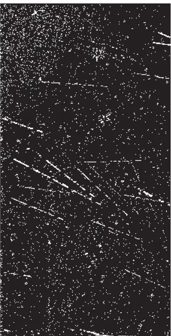
The second method is automatic. The routine begins by subtracting the bias and taking into acount the flatfield for each exposure. It then goes through each exposure, pixel by pixel, and identifies the
Figure 2: Image stacked within a 70 min total integration time, obtained with the automated method.
To detect the asteroids, we take into account each exposure and subtract the known stars using the PSF model. . We also subtract a smooth model of the background. Then we convolve the exposure with the expected size of an asteroid (3x5 pixels), in order to highlight detections that have the anticipated shape. We make a list of detections that are a minimum distance from known stars and are more significant than a given threshold The observed trails described by the moving object are measured and the positions of the moving object in pixels are reported.
As a second step, we measure the trails. This task is far from being easy, just because the fact that we see the trails does not mean that the computer can identify them. This task is realized through a statistical analysis of the residual stack image (stack image realized at the previous stage). We are now able to measure the trails, and measure the velocities in pixels/s in both x and y directions.
3
Astrometric calibration
Once the objects have been identified and their positions have been measured in pixel count, we proceed to the astrometric calibration. For that purpose we use the GAIA-GBOT (Ground Based Optical Tracking)
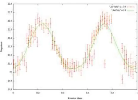
Figure 3: Asteroid light-curve obtained during the SMBAS-III session
PIPELINE (Bouquillon et al.,2012). It is devoted to the optical tracking of the GAIA mission in order to fully attain its goal in terms of astrometric precision. The expected astrometric accuracy is of 20mas with respect to the stars in the background field, which corresponds to 150 m for the position on the orbit of GAIA.
The pipeline uses the PPMXL star catalog (Roeser et al.,2010) as reference. The astrometric calibra-tion consits at first to go through all the exposure images, one by one, and to detect the sources brighter than a defined threshold. Then, once the sources have been identified, we extract the positions of the centroids in pixels, as well as the corresponding fluxes. When this step has been completed, we download, from the PPMXL astrometric catalog, the stars corresponding to the field of view of the observation (this information is retrieved through the header of the fits files). Then we connect the sources found in the field to those given by the catalogue. Therefore it is possible to redetermines the scale and the parameters of transformation matrices for astrometric reduction. Once applied to our data, the scale was found to be 201.996 mas/pixel which is really close to the theoretical value of 202 mas (Miyazaki et al.,2002).
4
Photometric-analysis using the GBOT-pipeline
One of our interests in analyzing the SMBAS-III data, is to study the size and taxonomic distributions of the identified populations (MBO’s, NEA’s and TNO’s) as well as to investigate the spin period dis-tributions of each of S-type and C-type groups by retrieving their light curves. For this purpose we use the GAIA-GBOT pipeline (Bouquillon et al.,2012), that was not initially destined for it. We proceed as follows : First we input the ephemeris of the asteroid (identified previously), by giving its initial position at the first epoch of detection in the field as well as its proper motion vector. This information is then updated into the .fits files headers.Second, as was done for the astrometric calibration (see the previous section), the stars in the field are identified and their positions and fluxes measured. The photomet-ric calibration is done by cross-identifying stars with the GSC2.3 photometphotomet-ric star catalog (Lasker et al.,2008) Then we go through all the exposures, one by one, and follow the target (the asteroid) reporting its position and measuring its flux, from which the magnitude can be computed.
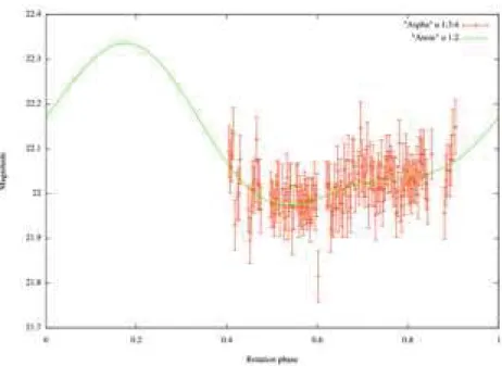
Figure 4: Asteroid light-curve obtained during the SMBAS-III session
heliocentric distance and the inclination with respect to the ecliptic) for each asteroid. We could deduce also significant light curves for very faint objects, as can be seen in Figs. X and Y. This work constitutes a part of D. Souami PhD thesis and the results will be gathered in papers with one related to the ACM meeting (Niigata, 2012) to come soon (Souami et al.,2012).
Acknowledgements This work is based on data collected at Subaru Telesocpe and obtained from SMOKA, which is operated by the Astronomy Data Center, National Astronomical Observatory of Japan (Baba et al.,2002)
References
Baba H., et al., 2002, ASPC, 281, 298
Bouquillon S., Taris F., Barache C., Carlucci T., Altmann M., Andrei A. H., Smart R., Steele I. A., 2012, LPICo, 1667, 6100
Bowell, E., Skiff, B. A., & Wasserman, L. H. 1990, Asteroids, Comets, Meteors III, 19. Dermawan B., Nakamura T., Yoshida F., 2011, PASJ, 63, 555
Lasker, B. M., Lattanzi, M. G., McLean, B. J., et al. 2008, AJ, 136, 735 Miyazaki S., et al., 2002, PASJ, 54, 833
Nakamura T., 1997, ceme.symp, 274
Nakamura, T., & Yoshida, F. 2008, PASJ, 60, 293 Nakamura, T., & Yoshida, F. 2002, PASJ, 54, 1079
Souami, D., Yoshida, F., Anderson, J., et al. 2012, LPI Contributions, 1667, 6061 Ouchi M., et al., 2004, ApJ, 611, 660
Roeser S., Demleitner M., Schilbach E., 2010, AJ, 139, 2440 Souami, D. PhD Thesis, 2012, in prep. (Dec. 7th., 2012)
Souami,D., Yoshida,F., Anderson,J., Nakamura,T., Dermawan, B., Yagi,M., Souchay,J., 2012, MAPS, submitted.
Yagi M., Kashikawa N., Sekiguchi M., Doi M., Yasuda N., Shimasaku K., Okamura S., 2002, AJ, 123, 66
Yoshida F., et al., 2001, PASJ, 53, L13
Yoshida F., Nakamura T., Watanabe J.-I., Kinoshita D., Yamamoto N., Fuse T., 2003, PASJ, 55, 701 Yoshida F., Nakamura T., 2004, AdSpR, 33, 1543
Yoshida F., Nakamura T., 2005, AJ, 130, 2900 Yoshida F., Nakamura T., 2007, P&SS, 55, 1113 Yoshida, F., & Nakamura, T. 2008, PASJ, 60, 297