Drag, turbulence, and diffusion in flow through emergent vegetation

Drag, turbulence, and diffusion in

flow through emergent vegetation

The MIT Faculty has made this article openly available.

Please share

how this access benefits you. Your story matters.

Citation

Nepf, H. M. “Drag, turbulence, and diffusion in flow through

emergent vegetation.” Water Resources Research 35.2 (1999): 479.

© 1999 American Geophysical Union

As Published

http://dx.doi.org/10.1029/1998WR900069

Publisher

American Geophysical Union

Version

Final published version

Citable link

http://hdl.handle.net/1721.1/68641

Terms of Use

Article is made available in accordance with the publisher's

policy and may be subject to US copyright law. Please refer to the

publisher's site for terms of use.

WATER RESOURCES RESEARCH, VOL. 35, NO. 2, PAGES 479-489, FEBRUARY 1999

Drag, turbulence, and diffusion in flow through emergent

vegetation

H. M. Nepf

Ralph M. Parsons Laboratory, Department of Civil and Environmental Engineering, Massachusetts Institute of

Technology, Cambridge

Abstract. Aquatic plants convert mean kinetic energy into turbulent kinetic energy at the

scale of the plant stems and branches. This energy transfer, linked to wake generation,

affects vegetative drag and turbulence intensity. Drawing on this physical link, a model is

developed to describe the drag, turbulence and diffusion for flow through emergent

vegetation which for the first time captures the relevant underlying physics, and covers the

natural range of vegetation

density and stem Reynolds' numbers.

The model is supported

by laboratory and field observations. In addition, this work extends the cylinder-based

model for vegetative resistance by including the dependence of the drag coefficient,

on the stem population density, and introduces the importance of mechanical diffusion in

vegetated flows.

1. Introduction

Freshwater and saltwater wetlands provide important tran- sition zones between terrestrial and aquatic systems, mediating exchanges of sediment [Phillips, 1989], nutrients [Nixon, 1980; Barko et al., 1991], metals [Orson et al., 1992; Lee et al., 1991], and other contaminants [Dixon and Florian, 1993]. Wetland plants control these exchanges both directly through uptake and biological transformation and indirectly by altering the hydrodynamic conditions [Kadlec, 1995]. The latter is the focus of this study, specifically the impact of vegetation on drag, turbulence intensity, and diffusivity. By providing a physically based model for estimating these parameters, the results of this paper will improve the engineering of wetland systems for wastewater and stormwater treatment, an increasingly popular and more environmentally sustainable alternative to tradi-

tional facilities.

The additional drag exerted by plants reduces the mean flow within vegetated regions relative to unvegetated ones [Kadlec,

1990; Shi et al., 1995]. This baffling promotes sediment accu- mulation by reducing near-bed stresses and subsequent erosion [Ward et al., 1984; Leonard and Luther, 1995]. An increase in drag can also lead to an increase in water depth and thus residence time, further influencing species' fate and biological activity [Jadhav and Buchberger, 1995; Kadlec, 1990]. Several efforts have been made to model the additional drag using a modified Manning's equation [e.g., Guardo and Tomasello,

1995]. Although useful for its simplicity, this adaptation of Manning's equation reveals little information about the flow structure within and above the canopy and cannot represent regions of emergent vegetation or regions of creeping or tran- sitional flow [Kadlec, 1990; Jadhav and Buchberger, 1995]. Other researchers have modeled vegetative drag based on cyl- inder drag, either using the drag coefficient as a fitting param- eter or choosing it on the basis of values for isolated cylinders as a function of Reynolds number [e.g., Burke and Stolzenbach, 1983; Hosokawa and Horie, 1992]. This paper extends the cyl-

Copyright 1999 by the American Geophysical Union.

Paper number 1998WR900069.

0043-1397/99/1998WR900069509.00

inder-based model by defining the effect of stem population density on drag coefficient. It can be applied across a range of flow conditions and for vertically varied vegetative density.

In addition to affecting the mean velocity, vegetation also affects the turbulence intensity and the diffusion. The conver- sion of mean kinetic energy to turbulent kinetic energy within stem wakes augments the turbulence intensity, and because wake turbulence is generated at the stem scale, the dominant turbulent length scale is shifted downward, relative to unveg- etated, open-channel conditions [Nepf et al., 1997]. The com- bination of reduced velocity and reduced eddy-scale should reduce the in-canopy macroscale diffusion relative to unveg- etated regions. This reduction has been observed for aquatic grasses [Worcester, 1995; Ackerman and Okubo, 1993].

This paper develops and tests a physically based model that predicts the turbulence intensity and diffusion within emergent vegetation. The model links vegetative drag, turbulence inten- sity, and turbulent diffusion. Observations of turbulence inten- sity match predictions based on the drag model. Observed diffusion rates, however, are greater than those predicted for turbulent diffusion alone. To explain the difference, this paper introduces the process of mechanical diffusion for vegetated flows. Together the contributions of turbulent and mechanical diffusion fully describe the observations. The newly described link between drag and turbulence intensity, as well as the introduction of mechanical diffusion as an important diffusive process in vegetated flows, can improve our understanding of seed and larvae dispersal in coastal marsh systems as well as our understanding of sediment and contaminant trapping. The results of this study are also relevant to the broader class of flow through distributed objects, for example, pesticide dis- persal within crops and pollutant dispersal within cities.

Section 2 introduces models for drag, turbulence, and diffu- sivity for flow through emergent vegetation. Laboratory and field experiments described in section 3 provide observations which support these models. The comparison of model predic- tion and experimental observation is given in section 4. Finally, the models are used to compare the mean flow, turbulence intensity, and diffusivity in vegetated and unvegetated regions (section 5).

2. Model Development

2.1. Drag Model for Emergent Vegetation

The drag force per fluid mass due to vegetation may be

described as

[force]

1 U2

Fr= massj

= 5 Cz>a

(1)

dh d

a = nd = AS2h

= AS2,

(2)

can define a dimensionless population density, ad - d2/AS 2.

For the cylinder model ad represents the fractional volume of the flow domain occupied by plants. Although it excludes the effects of stem morphology and flexibility, this model provides a reasonable first step for exploring the effect of vegetation density on drag.

The drag coefficient for an isolated element, Co, is affected by the wake structure, and thus depends on the Reynolds number, Red = Ud/v, where v is the kinematic viscosity. In coastal and freshwater systems Re d - O(1-1000) [Leonard and Luther, 1995; Hammer and Kadlec, 1986], a range which

covers both laminar and turbulent wake structure. Williamson

[1992] describes the details of this laminar to turbulent tran- sition for an isolated cylinder in a uniform flow. The cylinder wake remains laminar up to Red • 200, although vortex shedding is initiated at Re d • 50. For Re d >• 200, vortex instability causes the wake to become turbulent. Lateral shear in the flow upstream of an isolated cylinder can delay the onset of vortex shedding to Re d = 200 [Tamura et al., 1980], and because vortex shedding is a precursor to wake instability [Wil- liamson, 1992], the transition to a turbulent wake will also be delayed. Within a cylinder array, Nepf et al. [1997; ad = 0.008-0.07] observed that vortex shedding was initiated at Re d - 150-200, and attributed the delay to shear associated with upstream wakes. However, as the array density declines (ad --> 0), the critical Red values should return to those of an isolated cylinder. From the above observations, the transition from laminar to turbulent wake structure within the array is expected to occur at Red • 200. As is discussed shortly, wake structure (laminar versus turbulent) is important in defining the contribution of the wake to turbulent kinetic energy and diffusion within the array.

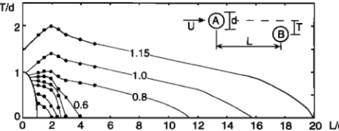
The bulk drag coefficient, Co, is a function of population density. To describe this relationship, we first consider the interaction of cylinder pairs. As summarized in Figure 1, ex- periments on pairs of cylinders have shown that the wake of an upstream cylinder can suppress the drag coefficient, Co, on the trailing cylinder for both semi-infinite [Bokaian and Geoola, 1984; Blevins, 1994] and finite cylinder lengths [Luo et al., 1996], where Co is based on the upstream velocity. This effect increases as both the lateral, T/d, and longitudinal, L/d, spacing between the cylinders decreases, and it results from two properties of the wake. First, the downstream cylinder experiences a lower impact velocity due to the velocity reduc-

06 0.8•

•

_,

0 2 4 6 8 10 12 14 16 18 2O L/d

Figure 1. Contours of drag coefficient, Co on trailing cylin- der, B, show the suppression of Codue to wake interaction. Contours are based on data measured with two cylinders (black dots [Bokaian and Geoola, 1984]) and on the observed decay of wake interference with separation distance [Blevins, 1994, pp. 177-181], which was used to set the longitudinal trend for the above contours between L/d = 6 and 20. Red = 2600, and Co- 1.17 at T/d, L/d -• •. A region of Co<

0 exists for L/d < 2, T/d < 0.25.

tion in the wake. Second, the turbulence contributed by the wake delays the point of separation on the downstream cylin- der, resulting in a lower pressure differential around the cyl- inder and thus a lower drag [Zukauskas, 1987; Luo et al., 1996].

Both of these wake characteristics contribute to the "shelter-

ing" effect described by Raupach [1992] that diminishes the drag on downstream elements.

Based on the observations for pairs of cylinders, we antici- pate that the bulk drag coefficient for an array, Cz>, will de- crease as the element spacing decreases or ad increases. To explore this trend, a numerical model was used to extrapolate the observations made for cylinder pairs [Bokaian and Geoola, 1984; Re d = 2600] to estimate the cumulative sheltering and bulk drag within a randomly arranged array. Cylinder place- ment within each numerical array was assigned using a random number generator with a placement resolution of d/10. For each cylinder i the local drag coefficient, Cz>i, was then as- signed based on the proximity of the nearest upstream neigh- bor. This assumes that changes in Cz>i are set by the strongest wake interaction (nearest cylinder) and neglects cumulative effects of multiple wake interaction. This is a reasonable as- sumption for sparse distributions, that is, ad < 0.1 [Raupach, 1992]. The total drag, Fr, was estimated as the sum of indi- vidual cylinder drags, and used with (1) to estimate Cz>. Fifty realizations were performed for each value of ad. The results,

presented later, indicate a strong dependence Cz>(ad) for

ad > 0.01. For comparison, several staggered array configu- rations were also considered. Although different in detail, the curves Cz>(ad) derived for the staggered arrays also show a decline in C z> within increasing ad.

2.2. Turbulence Intensity Within Emergent Vegetation

Even for sparse populations of emergent vegetation, the production of turbulence within stem wakes, Pw, exceeds the production through bed shear, Ps, over most of the flow depth [Nepfet al., 1997; Burke and Stolzenbach, 1983]. On the basis of this and the further assumption of homogeneity, the turbulent kinetic energy budget is reduced to a balance between the wake production and the viscous dissipation, e, that is, Pw • e. This simplification is confirmed experimentally, as discussed shortly. The wake production is estimated as the work input, FrU, where Fr is described in (1), that is, per unit mass:

NEPF: DRAG, TURBULENCE, AND DIFFUSION 481

OoøoO

^,_-o

",--0ø

m t

• •

0 '•

• '"'-"' /AYB

Figure 2. Mechanical diffusion arises from the physical ob- struction of the flow by stems. When a stem is encountered the

particle

must move

laterally

Ay -- d. For a large number

of

particles released at t - 0, and after many such encounters, the distribution of particles at time t is Gaussian with variance, o a • [ad]Udt, describing a Fickian diffusion process.

1

Pw

= 5 Cz)aU3

(3)

This assumes that all of the energy extracted from the mean

flow through stem (cylinder) drag appears as turbulent kinetic energy. This assumption is limited below Rea < 200 where the viscous drag, which dissipates mean flow energy without gen- erating turbulence, becomes increasingly important. As the fraction of viscous drag increases, Pw decreases from the value

given in (3).

Assuming the characteristic length scale of the turbulence is set by the stem geometry, that is, d, the dissipation rate will scale as

S • k3/2d -1, (4)

where k is the turbulent kinetic energy per unit mass [Tennekes and Lumley, 1990, p. 68]. Equating this with (3), the turbulence

intensity is given by

x•_ a•[C•ad]U3

(5)

where a• is an O(1)-scale coefficient. Thus the turbulence intensity increases with bulk drag coefficient and with popula- tion density. Note that because C D is a decreasing function of

population

density,

ad, the turbulence

intensity,

x/k/U, asso-

ciated with wake production may be considered a function of ad alone.

2.3. Diffusion Within Emergent Vegetation

The net diffusion within a cylinder array is determined by

two processes, turbulent and mechanical diffusion. Assuming a

turbulent Prandtl number of 1, the turbulent diffusivity may be

written as

D t-- ol2

x/•d,

(6)

where again the characteristic length scale of the turbulence is set by cylinder (stem) diameter [Nepf et al., 1997]. The velocity scale, X/•, and thus the turbulent diffusivity is linked to the array drag through (5). Because the array diffusivity is not isotropic [Nepf et al., 1997], the scale factor, a2, will differ

between horizontal and vertical diffusion.

Mechanical diffusion, D m, is common in porous media flow and reflects the dispersal of fluid particles due to variability in individual flow paths imposed by the tortuousity of the pore

spaces.

As shown

in Figure

2, this concept

can be extended

to

vegetated flows as the obstruction of the flow by stems creates similar variations in flow path. Consider particles released at (x, y) - (0, 0) that advect through the array at a mean velocity, U. For simplicity assume that advection dominates diffusion in longitudinal transport such that in each time in- terval, At, the particles move downstream a distance, Ax - UAt. In the same time, each particle has probability [aAx] of encountering a stem, and if a stem is encountered the particle is forced to move right or left along the y axis a distance Ay - •3d, where •3 is an O(1)-scale factor. On average and after many such collisions the particles move right and left with equal probability. After N steps, where N is large, the lateral (y) position of an individual particle is given by a Gaussian probability distribution with variance;

o-2= [aAx](13d)2t/At = 132[ad]Sdt (7a)

[Hoel et al., 1972]. For a large number of particles this model describes a Fickian diffusion process for which the variance of the particle distribution increases linearly with time, such that

the effective diffusion coefficient may be taken to be

Dm

= -•- [ad]Sd.

(7b)

Because the processes of mechanical and turbulent diffusion are independent, their variances, and thus their contribution to the total diffusivity, are additive. The total horizontal diffusiv-

ity is then given by

D =a[Cz•ad]U3+

[-•]ad, (8)

Ud

in which the net diffusivity has been nondimensionalized using the mean velocity, U, and cylinder diameter, d. The scale factor a = a•a 2 combines those appearing in (5) and (6).

3. Methods

3.1. Laboratory Experiments

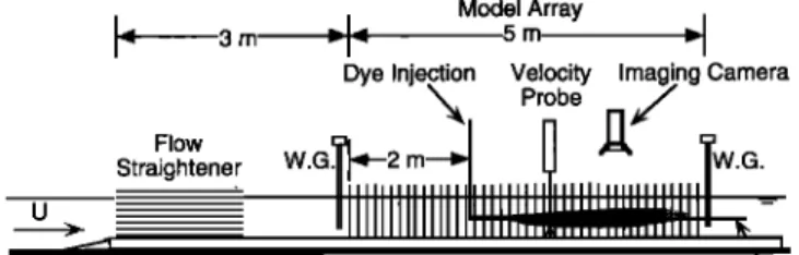
Laboratory experiments were conducted in a 24-m-long by 38-cm-wide, glass-walled flume with a flow depth h = 15 cm, shown in Figure 3. Model arrays were constructed from 1/4 inch (0.64 cm) wooden cylinders at densities between a - 1.2

and 10.5 m -• (at/ = [0.008-0.07], and equivalent

to 200-

J•

3 m

Flow

Straightener

Model Array

•11•

5 m

Dye Injection Velocity Imaging Camera

•, Probe .7

, _:t

I

Horizontal

Light

Sheet:

Position

of

Imaging

Plane--•

Figure 3. Laboratory experiments were conducted in a 5-m- long model array fitted into a 24 m recirculating flume. A continuous dye release was used to observe the horizontal diffusivity at mid-depth. The diffusivity was estimate by fitting the lateral profiles of mean concentration at multiple longitu-

dinal stations to the theoretical Gaussian distribution. Velocity

was measured using both acoustic Doppler (ADV) and laser Doppler (LDV) techniques. Surface slope through the array was measured using two 0.2 mm resolution wave gauges (WG).

2000 stems

m-2). The densities

were selected

based

on actual

stem populations observed in saltwater [Gambi et al., 1990] and freshwater environments [Kadlec, 1990]. The cylinders were mounted into half-inch (1.3 cm) Plexiglas boards and cut long enough to protrude through the water surface. The dowels were arranged randomly using a lm template generated by the numerical program described above. The template was applied five times, end to end, to create the total test section array of 5 m length. The array extended from wall to wall to prevent

accelerated currents close to the wall. The base boards ex-

tended 3 m upstream of the array and were tapered to the bottom to eliminate flow disruption. Smooth inlet conditions were achieved using mats of rubberized fiber to dampen inlet turbulence, and a 0.5 m section of honey comb to eliminate

swirl.

The velocity components (u, v, w), corresponding to streamwise, lateral, and vertical directions, respectively, were measured within the array using a 3-D acoustic Doppler velo-

cimeter (ADV) and a 2-D laser Doppler velocimeter (LDV) at

a cross section positioned at the mid-length of the array. A longitudinal transect through the array demonstrated that this position was representative of uniform flow conditions, that is, not affected by the leading edge. Six-minute records were collected at 25 and 100 Hz for the ADV and LDV, respec- tively. While the ADV could be deployed without disturbance to the array configuration, the LDV typically required the displacement of two or three dowels to clear its optical path. Because the flow field within an array is inhomogeneous at the scale of the array elements, a horizontal average is necessary to represent the mean, homogeneous (in x and y) velocity statis- tics [Kaimal and Finnigan, 1994, pp. 84-85]. Profiles were measured at five lateral positions for each flow condition. The mean and turbulent velocity statistics were then averaged lat- erally to find the representative, homogeneous values [Nepf et al., 1997]. The integral time scale, T u, was evaluated from the autocorrelation function and multiplied by U to form the Eu- lerian integral length scale: L u = UT u. The rate of turbulent dissipation, s, was evaluated from the velocity spectra, Suu, using the inertial subrange

18/32/3I

// ]2/3œ-5/3

Suu=A

,

where A • 1.5 is an experimentally determined, universal constant for turbulent flows [e.g., Kundu, 1990, p. 441]. As an example, Figure 4 shows a spectrum measured at mid-depth

within the dowel array with U = 5.5 cm/s and a - 2.8 m -•.

Note that the spectrum "levels" between 1 and 4 Hz, indicating a local-scale input of energy, here vortex shedding and wake production. For a single cylinder with d - 0.6 cm and U = 5.5 cm/s the shedding frequency falls atfs - 1.8 Hz. However, the shedding frequency is affected by the proximity of other cylinders within the array, potentially doubling as the cylinder spacing decreases [Weaver, 1993]. Thus a range of shedding frequencies (here, 1.8-3.6 Hz) is observed within the random array, reflecting the range of local array densities and its im- pact on shedding frequency. For higher velocity cases this wake-scale signature is pushed to higher frequencies. For these cases the sampling rate was increase to 100 Hz (using the LDV) to resolve this signature. Finally, the vertical turbulent transport, T = O(w'k)/Oz, and bed-shear production, Ps =

-u'w'(OU/Oz), terms were also evaluated from individual velocity records and then averaged laterally. The wake produc- tion was evaluated from (3).

Suu [cm 2 s] 101 lo o 10 -1 10 -2 Frequency (s -1)

Figure 4. Velocity spectrum, S, for U = 5.5 cm/s and a =

0.028 cm -•. Leveling of spectrum between 1 and 4 Hz corre-

sponds to stem-scale generation. An inertial sub-range fit, solid line, is used to estimate dissipation rate.

A pair of resistance-type surface displacement gauges (0.2 mm resolution), positioned 5 cm upstream and downstream of the array was used to measured the surface slope, O h/Ox, across the entire array. The bulk drag coefficient, Co, was then evaluated using the following force balance:

1 (•_) Oh

(1 - ad)CBU

2 + 5 CDad U

2= gh Ox'

(9)

where the first term on the left is the drag contributed by the base of the array, with a bed drag coefficient, C B = 0.001 [e.g., Munson et al., 1990, p. 673], the second term on the left is the drag contributed by the stems, and h is the flow depth. The drag contributed by the glass walls is negligible and dropped from (9) for simplicity.

The horizontal diffusivity was estimated using a continuous plume of dye released through a 0.16 cm (1/16 inch) stainless steel tube at mid-depth, midwidth, and 2 m from the leading edge. The injection velocity was carefully matched to the am- bient flow to avoid jet-induced mixing. The vertical centerline of the evolving dye plume was illuminated by a laser light sheet which caused the dye to fluoresce with an intensity propor- tional to the dye concentration [Monismith et al., 1990]. Video images of the plume were recorded and then transferred frame by frame to an image analysis software package using a frame

grabber. Using a 100-frame average, the mean lateral concen-

tration profile was recorded at multiple longitudinal positions from 20 to 100 cm downstream of the injection point. For the highest density array only, it was necessary to remove three to

five dowels at each measurement section to allow sufficient

penetration of the light sheet. Finally, in regions for which the lateral variance of the plume increased linearly in x, that is,

O

O'2/OX

= constant

(Fickian

diffusion),

the diffusivity

was

es-

timated by fitting the averaged profiles, containing 150-200 points, to the theoretical Gaussian plume profile [e.g., Fischer, 1979, chap. 2]. Although not discussed in this study, the vertical diffusivity was similarly estimated using a vertically orientated light sheet. These results are discussed by Nepf et al. [1997].

3.2. Field Experiments

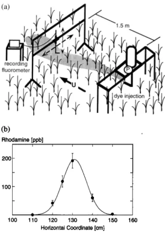
A similar dye plume technique was used to measure diffu- sivity in the field within an emergent stand of Spartina alterni- flora (smooth cordgrass) in the Great Sippewisset Marsh, Cape

NEPF: DRAG, TURBULENCE, AND DIFFUSION 483 (b) Fthodamino [ppb] i 200 - _ 100 - 1 1 O0 110 120 130 140 150 160 Horizontal Coordinate [cm]

Figure 5. (a) Field experiment at Sippewisset Marsh, Cape Cod. Dye injected at a continuous rate is measured 1.5 m downcurrent using a continuously recording, flow-through flu- orometer. The sampling port is traversed horizontally to mea- sure the plume concentration profile. (b) Determination of diffusivity from field data using exponential fit. Concentration at each point is averaged over 1 min. U - 5.5 cm/s, a = 2.1

m -• and D = 0.73 cm 2 s -• , ß

positions spaced at 10 cm across the mid-depth of the plume. At the start of each position 30 s were needed to fully purge the lines, this data was later removed before further analysis. The average concentration at each position was determined from 1 min of sampled data, the shortest time for which mean statis- tics were stable. The sampling time was constrained by the need to complete the profile within a period of steady current. The current speed was estimated before and after each profile was completed, by measuring the transit time of a small patch of dye injected at mid-depth across a short, fixed distance. The measurement was repeated 10 times for each estimate. Over the several field trials a range of velocity conditions were ob- served, with U = 3.0-7.4 cm/s andrea = 200-600. Finally, the diffusivity was determined by fitting the measured profile points to a Gaussian distribution using at least squares tech- nique. An example of this fitting procedure is given in Figure

5b.

4. Results

4.1. Laboratory Observations of Bulk Drag Coefficient

Figure 6 presents the model results, Cz>(ad), for both ran- dom (solid line) and staggered arrays (dashed line). The grey shading represents one standard deviation around the mean for the random array. Three configurations of staggered array were considered, defined by n, the ratio of the longitudinal to lateral spacing between success rows. For both random and staggered arrays the model predicts relatively constant values of C z> up to ad • 0.01 and a steady decline beyond this density. In general, the bulk drag coefficient drops off more rapidly for the staggered arrays. This reflects the fact that wake sheltering is strongest and persists for the greatest longitudinal spacing when the cylinders are aligned, that is, T/d = 0 in Figure 1. This alignment occurs intrinsically in staggered ar- rays, between every m th row, but only stochastically in random

arrays.

Cod, Massachusetts. This grass has a simple cylindrical-like morphology, and under normal tidal conditions exhibits only limited bending. Thus the stems and leaves resemble the cyl- inder array on which our model and laboratory experiments were based. The stem density was varied through pruning to

observe conditions at three values, n - 96, 196, and 370

stems

m -2. The stem density

was determined

by randomly

casting

a 0.1 m 2 frame over the vegetation

and counting

the

number of stems within the frame. This was repeated five times

for each condition. In addition, 100 stems were collected from

the site to determine an average leaf count (3.2 +_ 0.3 leaves per stem) and width (d = 0.69 _+ .03 cm). These character- istics were then used to estimate the vegetation density, a - 2.1, 4.3, and 8.2 m -•.

The tracer was prepared by mixing 2 mL of a 20% Rhoda- mine dye solution with 10 L of marsh water. A portion of the

solution was saved for later calibration. The solution was re-

leased through a 1/4 inch L tube at mid-depth (h • 1 m) and at the ambient flow speed using a variable-speed pump. As shown in Figure 5a, the dye injection table was oriented with its long axis (2 m) perpendicular to the current to eliminate the interference from the legs. The plume concentration was mea- sured 1.5 m downstream using a recording fluorometer in con- tinuous flow mode. While the concentration was continuously sampled at 10 Hz, internally averaged, and recorded at 1 Hz, the sample port was progressively moved to six horizontal

1.6 ... , ... ' " ' ' o o o

1.2

,--•,-'-•,•--o__•.-,... o

•..

ø .,

0.8

n= 112 1 2

0.4

10-3

10-2

1•0-1

Figure 6. Wake interference model predicts that the bulk drag coefficient, C z>, decreases with increasing array density, ad, for both random (solid line) and staggered (dashed lines) arrays. The data also represent both staggered (open symbols) and random (solid symbols) arrays. A summary of data sources, flow conditions, and symbols in given in Table 1. For the staggered arrays pitch is defined by n - ratio of longitu- dinal to lateral row spacing, that is, n - 1 is a square staggered

Table 1. Summary of Reynolds Number and Array Configuration Source R e a Configuration

Dunn et al. [1996] 1,000-4,000 staggered, n = 1/2 Seginer et al. [1976] 1,000 staggered, n = 1 Kays and London [1956] 1,000 staggered, n = 1-3

Petryk [1969] 10,000 random

staggered, n = 1, 2

Zdravkovich [1993] 1,000 staggered, n - 1'

Present study 4,000-10,000 random

Model >•200 random

staggered, n = 1/2-2 Here, n is ratio of longitudinal to lateral row spacing within staggered array. *One third, 2/3, and fully staggered.

Symbol in Figure 6 open circle open diamond square solid diamond triangle

square with slash

solid circle solid line dashed lines

The model results are compared to laboratory observations made in this study, as well as to a collection of other studies in both random and staggered arrays. A summary of the Reyn- olds' number and array configuration for each study is given in Table 1. Note that for Dunn et al. [1996], the rods are sub- merged, but that the drag coefficient, C z•B in that study, is defined on the basis of a vertical average over the height of the array only and so is roughly equivalent to Cry. For all other studies the cylinders extend through the entire flow domain, equivalent to an emergent condition. A reasonable agreement between the model and the experimental data is observed, even for ad > 0.1 for which the assumption that the nearest upstream cylinder alone sets degree of wake sheltering may be violated [Raupach, 1992]. The agreement between model and data suggests that the suppression of Cz• is correctly described by the wake shelter effects on which the model is based. Fi- nally, although values of large ad were included for model comparisons, the relevant range for aquatic vegetation condi- tions is ad = [0.001-0.1].

4.2. Laboratory Observations of Turbulence Structure

The assumptions made earlier regarding the production and the scale of turbulence within the array were confirmed by observation. First, within the array the Eulerian integral length scale, L•,, was fairly uniform over depth with L u/d • 1.5, L•, • 1 cm (Figure 7a). This value is diminished from that ob- served for unobstructed flow in the same channel, L•, = 5-6 cm, and supports the assumption that within the array turbu- lence is rescaled to the obstruction geometry, that is, d. Con- sistent with this, there is an excellent agreement between the spectrum-based estimates of dissipation rate and those based on the scale assumption t• - d (e.g., Figure 7b). Here, the dissipation rates are normalized by an equivalent shear veloc-

ity, Um= [ #h (dh/dx)

] •/2, and the flow depth.

Figure 8 shows the calculated terms from the turbulent ki- netic energy budget. The dissipation rate, s, and the wake production, Pw, are nearly constant over depth and balance one another, while the bed-shear production, Ps, and turbulent transport, T, terms are negligible except very close to the bed. These observations further support the assumption that turbu- lence levels are controlled by the balance of wake production and dissipation. For comparison, the boundary-layer scaling, s

• Um3/(gZ),

is also

included

(solid

line). It underpredicts

the

dissipation rate except close to the bottom where bed-shear production, Ps, increases to compete with Pw. In both Figures 7 and 8 constraints of the facility did not permit measurements above z/h > 0.8.

Finally, the dependence, suggested by (5), of the turbulence intensity on the dimensionless parameter, C z• ad, is confirmed in Figure 9. The values shown are depth-averaged turbulence intensity, excluding regions near the bed for which P• was non-negligible. From the data, a• = 0.9 _+ 0.1, in (5), with 95% certainty.

4.3. Diffusion: Laboratory and Field Observations

Figure 10 compares laboratory observations of diffusivity for

conditions with and without turbulent wakes. As described

above, the existence of laminar wakes was confirmed by the absence of vortex shedding. The dimensionless diffusivities observed for conditions producing turbulent wakes (open cir- cles) are more than an order of magnitude greater than those observed for laminar wakes (solid circles), and this difference is attributed to enhanced mixing after the onset of wake tur-

bulence. z/h 1 0.5 - (a) (b) L/d u I I

E, k 3/2

/ d

[F_.,

k 3/2/d

] [h / U 3]

Figure 7. Observations verify that the turbulence length scale, e, is set by the stem geometry, that is, e --- d. (a) The Eulerian integral length scale normalized by the cylinder di- ameter. (b) Estimates of dissipation rate based on the scaling e --• d (circles) match the observed dissipation rate (squares) based on spectrum fit. Dissipation estimates are scaled on an

equivalent

shear

velocity,

U m -- [#h(dh/dx)] •/2, and the

NEPF: DRAG, TURBULENCE, AND DIFFUSION 485 Z/h 1 0.8 0.6 0.4 0.2

Pw -

œ

•:(z/h)'

[Ps'

Pw'

T,

•][h/Urn

•]

,P

s

Figure 8. Selected terms from the turbulent kinetic energy

budget

for a - 2.8 m -•. Dissipation

rate, e, (triangles)

and

wake production, Pw (squares), balance over most of the flow depth. Bed-shear production, Ps (diamonds), becomes impor- tant near the bed. Vertical transport of turbulent kinetic en- ergy, T (circles), is negligible over the entire depth. See Figure

7 for normalization.

Boundary-layer

scaling,

e --- U3m

(•Z)- 2,

is included for comparison (solid line).

The dashed lines in Figure 10 indicate the two components of diffusion, turbulent (dashed-dotted) and mechanical (dashed), given in (8); the solid line indicates the sum of these two processes. The curve representing turbulent diffusion is based on (5) and (6) and incorporates the dependence Cr•(ad). The scale factor a• = 0.9 (in (5)), is based on direct experimental observation (Figure 9). The second scale factor, ot 2 in (6), was then selected to best fit the observed diffusion for the lowest values of ad, when mechanical diffusion is negligible (or 2 -- 0.9). The curve representing mechanical diffusion, (7b),

uses the assumed scale factor, /3 = 1. The data for laminar

wakes (Res - 60-90) generally. fall above this line, and this may be attributed to the presence of bed-generated turbulence even in the absence of vortex shedding. Alternatively, note that for/3 = 2, also a reasonable scale assumption, the mechanical diffusion line falls directly through the middle of the laminar wake observations (solid circles). Finally, the addition of the

•k/U 0.4 0.3 0.2 0.1 0.01 0.1

adC

Figure 9. Turbulence intensity within the stem array in- creases to the 1/3 power of the dimensionless parameter, Cr• ad, as predicted by scaling arguments, Pw "' •. Res = 400-

900. D/Ud 0.1 0.01

T'otal

DiffL•sion

=

i

•

/ Turbulent

/

Eqs..

5 & 6

/•

•i =0.9

/

o:2 =0.9

/

Eq.

7, [• =1

10 -2

10-•

Figure 10. Dimensionless diffusivity from laboratory obser- vations within two wake regimes, Res - 400-2000 (open circles) and Res = 60-90 (solid circles), fitted to model curves for mechanical (dashed line) and turbulent (dashed-dotted line) diffusivity, as well as the sum of both diffusion processes (solid line). Field data, Res = 300-600 (triangles), also fit the

model well.

mechanical and turbulent diffusion curves fits the turbulent

wake observations well (open circles), confirming the theoret- ical description.

The diffusivity measured in Sippewisset Marsh (Red = 300-600; Figure 10, triangles) is consistent with both the laboratory data and the model for turbulent wake conditions, although the Re d in the field were on the low end of those

observed in the lab. The normalized diffusion increases with

vegetation density with a slope which matches the local slope of the diffusion model. The average field diffusivities exceeded the laboratory values by •30%. This may be attributed to additional sources of turbulence present in the field, for exam- ple, wind, or to differences in morphology. However, the gen- erally good agreement between the laboratory (cylinder mor- phology) and the field data supports the use of this model for the marsh grass Spartina alternifiora. The model should also work well for other simple morphology, such as reeds. For more complicated stem morphology the relation Cr•(ad) re- quires more detailed evaluation, after which the model pre- sented here provides the basis for characterizing turbulence and diffusivity.

5. Discussion

5.1. Comparison of Vegetated and Unvegetated Flow

Conditions

The model developed above characterizes drag, turbulence, and diffusivity for flows through emergent vegetation. This model will now be used to compare hydrodynamic conditions in a region of emergent vegetation with conditions in an equiv- alent region of unvegetated, open-channel flow, denoted using subscript o. There are two key results of this comparison: (1) Turbulence intensity increases with the introduction of sparse

vegetation, but then decreases as stem population increases further. (2) Diffusivity within the vegetated system is consis- tently less than in the equivalent unvegetated system, owing principally to the decrease in eddy scale caused by the presence of the vegetation.

First, we consider the mean flow. The steady velocity, U, driven by a free-surface gradient is determined from the force balance given in (9). For simplicity, it is assumed that Ca is not affected by the presence of vegetation; that is, Ca is the same in both the vegetated and unvegetated systems. This assump- tion is not strictly correct, as the ratio of bed-friction velocity to mean flow speed, u ,/U, increases slightly with ad [Nepf et al.,

1997],

such

that Ca = (u,/U) •/2 also

increases

slightly

with

vegetation density. Two values of bed-drag coefficient, Ca = 0.001 and 0.005, equivalent to friction factors, f = 0.008- 0.04, are selected to represent conditions of smooth and rough earthen beds. The open-channel condition, Uo, is given by (9)

with ad - 0.

The depth-averaged turbulent kinetic energy, k, reflects two production terms, the bed shear and the wake production. When wake production dominates the turbulent kinetic energy is given by (5). When bed-shear production dominates, the

turbulent

kinetic

energy

is given

by, k •/2 "• CaU 2 [e.g.,

Nezu

and Rodi, 1986]. Combining these produces the scaling equa-

tion k- (1 - ad)CB U2 q- [Coad]2/3U 2 (10) lOO lO k/k o D/D o 0.1 0.01 10-5 /:J k/k • f(h/d)t • ... :..::.----.•. ... y.jz...•... ... :..

i i i i• i , , • •,,, , , , , ,,,,/

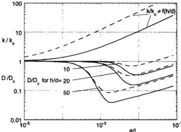
Figure 11. Comparison of turbulent kinetic energy, k, and diffusivity, D, for vegetated and unvegetated (subscript o) flow

conditions with the same velocity. Ca - 0.005 (solid lines)

and 0.001 (dashed lines). The curves represent qualitative trends only. The turbulence ratio, k/ko, increases steadily with stem population, at/, reflecting the contribution of wake pro- duction. The diffusion ratio, D/Do, is affected by reduction in eddy scale, and so is a function of the ratio of flow depth to vegetation scale, h/d.

(the terms to the left of the plus sign represent bed-shear production; those to the right represent wake production) which is correct in the limits of ad(-• 0 or 1) but may be oversimplified when the two terms are comparable because it

does not account for nonlinear interactions between the two

processes, for example, changes in bed shear arising owing to the presence of stems. Assuming that C z• = 1, wake produc- tion dominates for ad > 0.001 and 0.01, with Ca = 0.001 and 0.005, respectively. The equivalent open-channel condition

is given

by (10) with ad - 0, that is, ko • CaUo

2.

Because turbulent and mechanical diffusion are indepen- dent Fickian processes, their contribution to total diffusion, D,

is additive, that is,

O '• kl/2e q- [ad]Sd.

(11)

The first term represents the turbulent diffusion scale, Dr,

defined

by the turbulent

velocity

scale,

k •/2, and a mixing

length scale, •?. Note that because k is given by (10), a scale relation, (11) is strictly a scale relation as well, so that for simplicity we have excluded previously defined scale factors. The second term in (11) represents the mechanical diffusion, D,•, based on (7b) excluding the scale factor, /3. The mixing length scale, •, depends strongly on the presence of vegetation. In unvegetated flow, •? and thus D t increase with the scale of the diffusing patch until the largest length scale is reached, that is, the length scale defined by the flow domain [Okubo, 1971]. In contrast, in vegetated flow the mixing-length scales on the vegetation geometry, • • d, for all patch sizes greater than d

[Nepf et al., 1997]. To evaluate (11), we set the following limits

on the mixing length. First, for simplicity we assume a mixing length, •o • h, for unvegetated open-channel flow (ad = 0). If only sparse vegetation is introduced to this flow, that is, vegetation with spacing AS > •o, the channel-scale eddies, •o, persist and continue to dominate the diffusive transport. Thus for sparse vegetation the dominant mixing length is still • = •o

= h. For dense populations, AS < e o, the stems break apart channel-scale eddies, reducing the mixing-length scale, until at at/> 0.01, I• • d [Nepfet al., 1997]. The model assumes that • varies linearly from h to d between these limits.

By using (9)-(11) the flow conditions in a vegetated channel

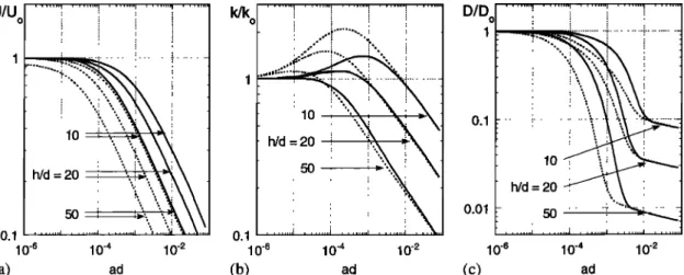
and an equivalent, unvegetated channel can now be compared. We consider three ratios of depth to stem scale, h/d = 10, 20, 50, to be representative of field conditions. Keep in mind that

(10) and (11) are scale relations, so that the parameters they

describe, D/Do and k/ko, respectively, provide only qualitative predictions of flow behavior.

For simplicity, we first consider the case for which the flow speed is the same in both the vegetated and unvegetated chan- nels, that is, U = Uo (Figure 11). For equivalent flow speed the turbulent kinetic energy ratio, k/ko, is greater than one for all values of at/> 0, and increases to O (10) at high vegetation density. This trend reflects the additional source of turbulence provided by the stem wakes. Even though k/ko > 1, D/Do -< 1 for most values of at/ (Figure 11). For sparse vegetation (small at/), D/Do • 1 despite the addition of wake-generated

turbulence. This occurs because eddies that are channel scale,

h, can persist in sparse vegetation (as described above), and because the additional turbulent kinetic energy is introduced at the stem scale, d << h. The larger, channel-scale eddies dom- inate the macroscale diffusive transport. The addition of small- er-scale mixing does, however, smooth out local gradients within the turbulent patch [Nepf et al., 1997]. As at/increases, the stems impinge on the channel-scale eddies, and these ed- dies are broken apart. All of the turbulence is then rescaled to the stem geometry. The reduction in eddy-scale causes the relative diffusion, D/Do, to decrease, even though the relative turbulence, k/ko, continues to increase. A similar trend was

observed in a channel flow downstream of a mesh. Turbulence

intensity was enhanced by the presence of the mesh, yet the diffusivity was diminished because the eddy scale was reduced

NEPF: DRAG, TURBULENCE, AND DIFFUSION 487 0.1 1 o.1 o.1 O.Ol 10 -6 10 '4 10 '2 10 '6 10 '4 10 '2 (a) ad (b) ad (c)

: 10 i

•:

Figure 12. Comparison of flow conditions within vegetated and unvegetated (subscript o) regions under the same forcing, that is, surface slope: (a) velocity, (b) turbulent kinetic energy, and (c) diffusivity. Bed drag

coefficients of 0.01 (solid lines) and 0.005 (dashed lines) are considered as well as three ratios of depth-to-stem diameter.

[Hinze, 1987, pp. 448-449]. In Figure 11 the decline in eddy scale is initiated at ad •- [0.002, 0.001, 0.0002] for h/d = [ 10, 20, 50], respectively. The transition occurs earlier (small- er ad) in larger flow depths, because the larger channel-scale eddies, e o '" h, are impacted at a larger stem spacing (AS). Once the vegetation is sufficiently dense (ad •- 0.01) the stem-scale turbulence dominates and e --- d. With the length- scale fixed, the continued increase in turbulence intensity with increasing ad produces an increasing D/Do. In addition, me- chanical diffusion becomes important at these high vegetative

densities.

In the above discussion (Figure 11), vegetated and unveg- etated flow conditions were compared using identical mean flow, U = Uo. For a more relevant but more complex com- parison, we now consider the two systems under identical forc- ing, that is, identical surface slope, Oh/Ox. The velocity, tur- bulence, and diffusion ratios for this condition are given in Figure 12. Because the vegetation offers additional resistance, the velocity within the vegetated channel is always less than that in the unvegetated channel, and the velocity ratio, U/Uo, decreases as the vegetation density (ad) increases (Figure 12a). The drop in velocity ratio is more rapid for greater flow depths and smaller values of bed friction, C B, both of which enhance the fractional contribution of vegetative resistance.

Changes in turbulent kinetic energy (Figure 12b) reflect the

competing effects of reduced velocity and increased turbulence production, both of which accompany the introduction of veg- etation. These opposing tendencies produce a nonlinear re- sponse in which the turbulence levels initially increase with increasing stem density, but eventually decrease as ad in- creases further. A similar response was predicted numerically for flow through emergent vegetation [Burke and Stolzenbach, 1983] and within bottom roughness elements [Eckman, 1990] and was observed in a flume study of flow through real stems of Zostera Marina [Gambi et al., 1990]. Note, however, that (10) and Figure (12b) exclude the contributions of turbulence generated by wind and wave action, which may be present in the field. Because emergent vegetation damps wave energy and shelters the water surface from wind stress, both of these pro- cesses would affect the ratio k/ko by more readily augmenting turbulence in open-channel regions than in vegetated regions.

The trends in turbulence intensity (kX/2/U) suggested by Fig-

ures 12a and 12b have important implications for canopy ecol- ogy. For example, an increase in turbulence intensity could benefit the vegetation by augmenting nutrient uptake and/or gas exchange [Anderson and Charters, 1982]. Within waste-

treatment wetlands the turbulence level can control the rate at

which contaminants are delivered to vegetation surfaces where degrading microbes live and thus may determine the rate of degradation [e.g., Gantzer et al., 1991]. Finally, increased levels of turbulence experienced at sparse plant density may explain why patchy plantings, unlike dense ones, do not promote the desired sediment accumulation for bank stabilization (J. Hart, personal communication, 1998), and may actually create higher rates of erosion [Coppin and Richards, 1990, p. 58].

The diffusivity ratio for identical surface-slope conditions (Figure 12c) again reflects the importance of reduced eddy scale within the vegetated region. As described above, a rapid decline in D/Do occurs once the stems impinge on the channel- scale eddies, and convert them to progressively smaller scales as at/increases. Once • --- d, for example, ad > 0.01, a more gradual decline in D/Do is observed, reflecting the near bal- ance between declining velocity ratio, U/Uo, and increasing contribution by mechanical diffusion, D m --- ad.

5.2. Reynolds Number Dependence

A majority of the above discussion describes conditions of Rea >• 200, for which Cr• is only a weak function of Rea [e.g., Munson et al., 1990, p. 614]. These conditions are com- mon in coastal systems such as the Sippewisset Marsh used in this study [also, e.g., Leonard and Luther, 1995]. However, conditions of Re a < •- 200 are also common in the field, in particular in freshwater systems which are not exposed to strong tidal flows. For Re a < •- 200 wake production is neg- ligible and the turbulent component of diffusion will be greatly reduced, determined solely by the bed shear (and possible wind shear). For these conditions, the total diffusion is likely dominated by mechanical diffusion. This study suggests that

mechanical diffusion alone is still sufficient to maintain mac-

roscale diffusion at levels above the molecular value. Finally, the removal of wake turbulence below Re a •. 200 also alters the dynamics of wake interference and thus the relation C r• =

f(ad). Further study is needed to understand bulk drag under

these conditions.

6. Conclusions

This paper presents a model for drag, turbulence and diffu- sion within emergent vegetation which captures the relevant underlying physics, and covers a natural range of vegetation density and stem Reynolds' numbers. This work also extends the cylinder-based model for vegetative resistance by including the dependence of the bulk drag coefficient, C z>, on the veg- etative density, ad, for Red > • 200. The model, confirmed by

experimental

results,

shows

that turbulence

intensity,

kl/2/U,

is principally dependent on the vegetative drag, and that for vegetative densities as small as 1% (ad = 0.01), the bed-drag and bed-shear production are negligible compared to their vegetation counterparts. The fraction of mean energy parti- tioned to turbulence depends on the ratio of form drag to viscous drag on the stems, which in turn depends on the mor- phology and flexibility of the stems, and the stem Reynolds number. In addition, the model predicts that turbulence inten- sity increases with the introduction of sparse vegetation owing to the addition of wake production but then decreases with increasing population density as mean flow speed is reduced. Because of the reduction in eddy scale, diffusion is reduced within an array. Specifically, for vegetative densities greater than 1%, turbulence scales are controlled by vegetation geom- etry, that is, I? --- d. The mixing-length scale, t?, is thus reduced from open-channel conditions, I? o --- h or larger. This shift in eddy scale controls the turbulent diffusion, such that turbulent diffusivity is reduced within the vegetated region, despite the fact that turbulence intensity may be increased. For higher vegetation density mechanical diffusion becomes important, that is, diffusion arising from the obstruction of direct flow paths by the vegetation (array elements), and will dominate the overall diffusion of scalar species for ad > O(0.1) or for Red

<• 200.

Acknowledgments. This work was completed under NSF CA- REER Award, EAR 9629259. The author would like to thank Becky Zavistoski, Jenn Sullivan, Al Tarrell, and Enrique Vivoni for their assistance with laboratory and field experiments; and both Ole Madsen and Dennis Lyn for providing thoughtful editorial comments.

References

Ackerman, J., and A. Okubo, Reduced mixing in a marine macrophyte

canopy, Functional Ecol., 7, 305-309, 1993.

Anderson, M., and A. Charters, A fluid dynamics study of seawater flow through Gelidium nudifrons, Limnol. Oceanogr., 27, 399-412,

1982.

Barko, J., D. Gunnison, and S. Carpenter, Sediment interactions with submersed macrophyte growth and community dynamics, Aquatic Bot., 41, 41-65, 1991.

Blevins, R., Flow-Induced Vibration, Krieger, Malabar, Fla., 1994.

Bokaian, A., and F. Geoola, Wake-induced galloping of two interfer- ing circular cylinders, J. Fluid Mech., 146, 383-415, 1984.

Burke, R., and K. Stolzenbach, Free surface flow through salt marsh grass, Tech. Rep. MITSG 83-16, Mass. Inst. of Technol., Cambridge,

1983.

Coppin, N., and I. Richards (Eds.), Use of Vegetation in Civil Engineer-

ing, Butterworths, London, 1990.

Dixon, K., and J. Florian, Modeling mobility and effects of contami-

nants in wetlands, Environ. Toxicology Chem., 12, 2281-2292, 1993. Dunn, C., F. Lopez, and M. Garcia, Mean flow and turbulence in a

laboratory channel with simulated vegetation, Hydraul. Eng. Ser., 51, Univ. of II1:, Urbana, 1996.

Eckman, J., A model of passive settlement by planktonic larvae onto bottoms of differing roughness, Limnol. Oceanogr., 35, 887-901,

1990.

Fischer, H. B., E. J. List, R. Koh, J. Imberger, and N. Brooks, Mixing

in Inland and Coastal Waters, Academic, San Diego, Calif., 1979. Gambi, M., A. Nowell, and P. Jumars, Flume observations on flow

dynamics in Zostera marina (eelgrass) beds, Mar. Ecol. Prog. Ser., 61,

159-169, 1990.

Gantzer, C., B. Rittmann, and E. Herricks, Effect of long-term water velocity changes on streambed biofilm activity, Water Res., 25, 15-20,

1991.

Guardo, M., and R. Tomasello, Hydrodynamic simulations of a con- structed wetlands in south Florida, Water Resour. Bull., 31,687-701,

1995.

Hammer, D., and R. Kadlec, A model for wetland surface water

dynamics, Water Resour. Res., 22, 1951-1958, 1986. Hinze, J., Turbulence, 2nd ed., McGraw-Hill, New York, 1987. Hoel, P., S. Port, and C. Stone, Introduction to Stochastic Processes,

Waveland, Prospect Heights, II1., 1972.

Hosohawa, Y., and T. Horie, Flow and particulate removal by wetlands with emergent macrophyte, in Marine Coastal Eutrophication Science

of the Total Environmental Supplement, edited by R. Vollenweider et

al., Elsevier Sci., New York, 1992.

Jadhav, R., and S. Buchberger, Effects of vegetation on flow through

free water surface wetlands, Ecol. Eng., 4, 481-496, 1995.

Kadlec, R., Overland flow in wetlands: Vegetation resistance, J. Hy-

draul. Eng., 116, 691-707, 1990.

Kadlec, R., Overview: Surface flow constructed wetlands, Water Sci. Technol., 32, 1-12, 1995.

Kaimal, J., and J. Finnigan, Atmospheric Boundary Layer Flows, Oxford

Univ. Press, New York, 1994.

Kays, W., and A. London, Compact Heat Exchangers, Natl. Press, Palo Alto, Calif., 1955.

Kundu, P., Fluid Mechanics, Academic, San Diego, Calif., 1990.

Lee, C. K., K. Low, and N. Hew, Accumulation of arsenic by aquatic plants, Sci. Total Environ., 103, 215-227, 1991.

Leonard, L., and M. Luther, Flow hydrodynamics in tidal marsh can-

opies, Limnol. Oceanogr., 40, 1474-1484, 1995.

Luo, S., T. Gan, and Y. Chew, Uniform flow past one (or two in tandem) finite length circular cylinder(s), J. 1,14nd Eng. Ind. Aerodyn.,

59, 69-93, 1996.

Monismith, S., J. Koseff, J. Thompson, C. O'Riordan, and H. Nepf, A

study of model bivalve siphonal currents, Limnol. Oceanogr., 35,

680-696, 1990.

Munson, B., D. Young, and T. Okiishi, Fundamentals of Fluid Mechan- ics, John Wiley, New York, 1990.

Nepf, H. M., J. A. Sullivan, and R. A. Zavistoski, A model for diffusion

within an emergent plant canopy, Limnol. Oceanogr., 42(8), 85-95,

1997.

Nezu, I., and W. Rodi, Open-channel flow measurements with a laser

Doppler anemometer, J. Hydraul. Eng., 112(5), 335-355, 1986.

Nixon, S., Between coastal marshes and coastal waters--A review of twenty years of speculation and research on the role of salt marshes in estuarine productivity and water chemistry, in Estuarine and Wet-

land Processes, edited by P. Hamilton and K. MacDonald, pp. 438-

525, Plenum, New York, 1980.

Okubo, A., Oceanic diffusion diagrams, Deep Sea Res., 18, 789-802,

1971.

Orson, R., R. Simpson, and R. Good, A mechanism for the accumu- lation and retention of heavy metals in tidal freshwater marshes of

the Upper Delaware River estuary, Estuarine Coastal Shelf Sci., 34,

171-186, 1992.

Petryk, S., Drag on cylinders in open channel flow, Ph.D. thesis, Colo.

State Univ., Fort Collins, 1969.

Phillips, J., Fluvial sediment storage in wetlands, Water Res. Bull., 25, 867-872, 1989.

Raupach, M., Drag and drag partition On rough surfaces, Boundary Layer Meteorol., 60, 375-395, 1992.

Seginer, I., P. Mulhearn, E. Bradley, and J. Finnigan, Turbulent flow in a model plant canopy, Boundary Layer Meteorol., 10, 423-453, 1976. Shi, Z., J. Pethick, and K. Pye, Flow structure in and above the various heights of a saltmarsh canopy: A laboratory flume study, J. Coastal

Res., 11, 1204-1209, 1995.

Tamura, H., M. Kiya, and M. Arie, Vortex shedding from a circular

cylinder in moderate-Reynolds-number shear flow, J. Fluid Mech., 141, 721-735, 1980.

NEPF: DRAG, TURBULENCE, AND DIFFUSION 489

Tennekes, H., and J. L. Lumley,i A First Course in Turbulence, MIT Press, Cambridge, Mass., 1990.

Ward, L., W. Kemp, and W. Boyton, The influence of waves and seagrass communities on suspended particulates in an estuarine embayment, Mar. Geol., 59, 85-103, 1984.

Weaver, D., Vortex shedding and acoustic resonance in heat exchanger tube arrays, in Technology for the '90's, edited by M. K. Au-Yang, pp. 777-810, Am. Soc. of Mech. Eng., New York, 1993.

Williamson, C. H. K., The natural and forced formation of spot-like "vortex dislocations" in the transition of a wake, J. Fluid Mech., 243,

393-441, 1992.

Worcester, S., Effects of eelgrass beds on advection and turbulent mixing in low current and low shoot density environments, Mar. Ecol. Prog. Ser., 126, 223-232, 1995.

Zdravkovich, M., Interstitial flow field and fluid forces, in Technology

for the '90's, edited by M. K. Au-Yang, p. 634, Am. Soc. of Mech. Eng., New York, 1993.

Zukauskas, A., Heat transfer from tubes in cross-flow, Adv. Heat Trans., 18, 87-159, 1987.

H. M. Nepf, Department of Civil and Environmental Engineering, Massachusetts Institute of Technology, Ralph M. Parsons Laboratory, Cambridge, MA 02139. ([email protected])

(Received May 6, 1998; revised October 21, 1998; accepted October 21, 1998.)