Directional impedance of geared transmissions

Directional Impedance of Geared Transmissions

by

Albert Duan Wang

S.B., Massachusetts Institute of Technology (2010)

Submitted to the Department of Mechanical Engineering

in partial fulfillment of the requirements for the degree of.., A

OFTCNOLOGY

Masters of Science in Mechanical Engineering

OCT

2 2

2012

at the

RIES

MASSACHUSETTS INSTITUTE OF TECHNOLOGY

September 2012

@

Massachusetts Institute of Technology 2012. All rights reserved.

,4'

/

I,

A uthor ...

Certified by ...

- - I V

. . ...

Department of Mechanical Engineering

August 24, 2012

8Lfgbae Kim

Mecha

al Engineering

hesis Supervisor

. . . .

Esther & Harold E. Edgerton Assistant Professor of

/ u~91

A ccepted by ...

.

. ...

David E. Hardt

Ralph E. & Eloise F. Cross Professor of Mechanical Engineering

Chairman, Committee on Graduate Students

Directional Impedance of Geared Transmissions

by

Albert Duan Wang

Submitted to the Department of Mechanical Engineering on August 24, 2012, in partial fulfillment of the

requirements for the degree of

Masters of Science in Mechanical Engineering

Abstract

The purpose of this research is to develop a design tool for geared actuation sys-tems that experience bidirectional exchange of energy with the environment. Despite the asymmetry of efficiency depending on the direction of power transfer in geared systems, typical dynamic models consider a fixed transmission efficiency for all con-ditions which can result in significant error depending on specific gear selection and the number of stages. This error can cause issues especially in dynamic legged robots and haptic devices when accurate force control is desired. In this paper we present directional impedance, a characteristic of geared transmissions in which the amount of power loss through the transmission differs according to the direction of power flow. Typical robots use electric motors with high gear reduction which introduces larger impedance when power flows from the output back to the motor than when the power flows from motor to output. To investigate the dependence on power flow direction, friction loss from gear teeth sliding in the gear mesh is modeled by a single gear tooth contact model and dynamic models are presented for each power transfer direction. Combinations of 0.5 mod gears were tested in experiment over a range of sizes between 16 and 120 teeth to characterize the directional effects over multiple gear selections. The experiments confirmed that for a set of differently sized gears, power loss is greater when the larger gear drives the smaller one than in the reverse case, and the asymmetry was up to 17% in the 16 and 120 tooth gear set. With a multiple stage gearbox, the difference in loss is further amplified. These findings show that directional loss in gears is a non-negligible effect and must be considered in both dynamic modeling and gear selection of robotic actuators. The gear loss model enables the modeling of motor and gearbox as a single package which can then be optimized for desired performance parameters such as peak torque, torque per mass, and mechanical impedance.

Thesis Supervisor: Sangbae Kim

Acknowledgments

I would like to thank my advisor Prof. Sangbae Kim for inspiration and insight during

this project. I'd also like to thank Sangok Seok and National Instruments for support with LabVIEW. Prof. Jeffrey Lang and David Otten of EECS helped with motor theory and control.

Contents

1 Introduction 13

2 Theory 17

2.1 Single Tooth Gear Contact Model . . . . 17

2.2 Dynamics of Lossy Transmissions . . . . 21

3 Gear Friction Experiment 25 3.1 Experimental Setup . . . . 25

3.1.1 Motor Driver . . . . 28

3.1.2 Motor Calibration. . . . . 30

3.2 Experimental Method. . . . . 31

3.3 R esults . . . . 32

3.4 A new loss model . . . . 32

3.4.1 Direction Impedance . . . . 34

4 Conclusion 37 4.1 Actuator Modeling . . . . 37

4.2 Actuator Design. . . . . 37

List of Figures

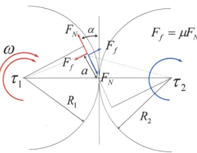
2-1 Force diagrams of single gear contact between two teeth. The sliding direction changes as the contact point moves past the centerline and the sliding friction force changes direction . . . . 19

2-2 Results of the single tooth gear friction model averaged over the line of action for several combinations of input and output gear sizes. All gears are 0.5 mod and 200 pressure angle. The sliding friction coefficient is

0 .3 . . . . 20

2-3 The force diagram of power flow from side 1 to side 2 through a set of gears. Loss is taken as a factor of torque entering the gear mesh that does not become amplified by the gear ratio. . . . . 23

3-1 Mechanical design of the experimental setup for testing gear friction . 26

3-2 _{Partially disassembled mechanical setup showing the two sets of plates,}

each holding a motor and driveshaft. . . . . 27

3-3 The distance between locating pins on each set of plates is used to precisely measure and set the spacing between the gears . . . . 27

3-4 National Instruments NI cRIO-9082 chassis showing the control elec-tronics. From left to right, the first three and last three slots house N19505 DC Brushed Servo Drive used to drive a single phase of a three-phase brushless motor. A LEM CASR 15-NP hall effect current sensor is mounted above each motor driver and measures the current in that phase. The fourth slot is a NI 9205 analog input module used to measure the output of the current sensors. Slot 5 is a direct digital connection to the two magnetic encoders on the motor shafts. . . . . 29 3-5 The block diagram of the control algorithm used in to drive the

brush-less m otors . . . . 30 3-6 Loss factors of different gear pairs obtained from experiment. . . . . . 32 3-7 The skew data plotted with the scaled theoretical model using

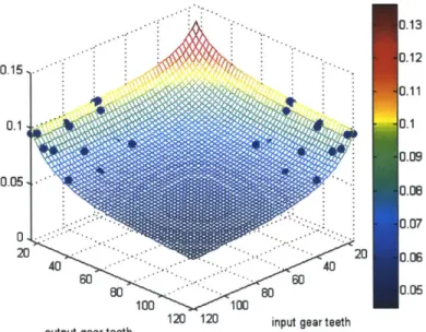
fric-tion coefficient u=0.5 and scaling the model by a factor of 100. The blue points are the skew components of the experimental data and the surface plot is the corrected model. . . . . 33 3-8 The symmetric data plotted with the theoretical model using friction

coefficient u=0.5 and adding a steady state component of 0.025. The blue points are the symmetric components of the experimental data and the surface plot is the corrected model. . . . . 34

List of Tables

Chapter 1

Introduction

Dynamic locomotion involves high acceleration through foot impact and alternating positive and negative work at each stride. The ability to produce correct ground reaction force depends on the actuators' mechanical characteristics. Particular to running robots and haptic displays, in which energy flows in and out of the ac-tuator, mechanical impedance must be considered which is directly related to the passive characteristic of the actuator called 'backdrivability' [10]. The performance of force controlled manipulators and haptic devices, often evaluated by the capability of achieving prescribed impedance or force trajectories, rely heavily on the character-istics of actuators' mechanical impedance in both power transfer directions. A large component of impedance arises from the use of gearing on electric motors in typical robots.

Electromagnetic rotary motors typically used in robotics tend to produce insuf-ficient torque for direct drive due to the thermal or magnetic field limits but they can achieve high power at high speed. As one of simplest and robust ways to obtain torque amplification and speed reduction, gearboxes are found in nearly all robotic actuators. They can transmit large torques and increase actuator torque per mass and torque per volume with greater flexibility than increasing motor size. Further-more, major motor manufacturers offer modular gearheads of several stages with gear reductions reaching 1000:1.

to the end effector but the gear ratio inevitably creates high impedance reflected at the end effectors. The inertia and damping on the motor shaft is reflected to the output shaft by a factor equal to the square of the gear ratio. The high impedance reduces the force transparency of the system as the motor cannot accurately sense the force put on the output shaft. For high force dynamics, there is a need for both a transparent transmission and an accurate model of how the forces are transmitted between the motor and end effector.

In addition to increasing the backdriving impedance of geared systems through reflected inertia and damping, the geared transmission itself adds impedance though friction. In highly geared systems, it is extremely difficult to backdrive the actuator. Although reflected dynamics play a role, the experiments presented in this paper show that gear friction acts asymmetrically depending on power transfer direction and increases the amount of power loss during backdriving than during times when power flows from motor to output shaft. This directional impedance phenomenon of has been considered in robotic arms and compensated by adding transmission efficiency factors and switching dynamics equations depending on the state of power transfer [11]. However, it is not widely known in robotics that the asymmetry always acts to increase loss in the backdriving direction due to the geometric contact of the gears. [5] showed a torque dependent directional friction model for worm gears but did not consider spur gears used in most robots. There have also been many attempts at gear friction modeling to provide accurate models for wear and energy efficiency purposes [7] [9] [6] [1]. However, these models ignore the directional impedance effects and only consider the loss of power in a single transfer direction such from the engine of an automobile to the wheels.

Detailed gear models have not been well studied in the context of the design of

highly dynamic robotics. Previous work does not provide quantitative models that

specifically allow for the design and optimization of mechanical impedance of actua-tors. In some robots, the complexities of gear behavior have been avoided altogether using direct drive from the electromagnetic actuator [2]. Most haptic robots minimize the effect of backdrive impedance by reducing gearing or decreasing friction by

em-ploying cable transmissions. While previous work attempted to reduce transmission dynamics, the amount of force that the robot can apply is limited. The fundamental trade off is between transmission backdrive impedance and available torque. Another method introduced in the MIT Cheetah [10] is to increase the gap radius of the motor, but it is not always possible due to space constraints. This paper attempts to unify a directional gear loss model with actuator dynamics in order to provide more accurate dynamic model of behavior. When combined with an electromagnetic motor model, the motor and gear parameters can be used to determine the tradeoffs between differ-ent performance metrics. It is then possible to optimize actuator performance with a cost function that weighs the desired characteristics.

Chapter 2

Theory

2.1

Single Tooth Gear Contact Model

The involute gear tooth profile is nearly universally because the kinematic constraints enforce constant angular velocity throughout rotation. Gear teeth transmit force along the line of action where the teeth mesh. In the analysis of gear mesh friction, we make assumptions about the contact. In most spur gear sets, the contact ratio is 1.2 or greater [4]. For low contact ratios less than 1.5, a majority of the contact time is between a single tooth on each gear. Similar to the models analyzed by Anderson

[1], we focused on Coulomb sliding friction between the tooth contact perpendicular

to the line of action. While not containing the same complexities as existing detailed models, the simple model can be used to explain the dynamic behavior of geared systems and provide insight on the design of actuators to meet dynamic performance specifications of future robots.

The force diagram of a gear mesh is shown in Figure 2-la. Assuming that the gears are moving at some non-zero velocity and the torques are the reaction on the gear from the shaft, the gear power loss at the output side gear soon after the driving gear tooth engages with the driven gear is shown below in Equation 2.1.

A pa(Ri + R2)

where p is the coefficient of sliding friction, a is the distance on the pitch line between the contact point and the center line between the two gears, R1 is the pitch radius of

the driving gear, R2 is the pitch radius of the driven gear, and a is the pressure angle

of the gears. This equation is valid along the line of action for values of a from 0 to

R2cos(ir/2 + a) + R

+

2 _(a)

- R in which R2,o is the outer radius of gear 2.

The direction of sliding between the gear teeth changes after the contact point crosses the center line and the equation for the torque loss factor changes slightly. The force diagram is depicted in Figure 2-la and loss factor is given equation 2.2 and is valid for a between 0 and Ricos(7r/2 + a)

+

A =pa(R 1 + R2)

R2(pa + Ricos(a) + pRisin(a))

An important observation is that the gear loss is not symmetric with power di-rection. That is, for each set of gears the loss is different depending on which gear is the driving gear. At any given point during contact, switching the power transfer direction is equivalent to switching between equations 2.1 and 2.2 and then switching R1 and R2. The instantaneous loss at each point along the line of action does not result in the same value for the reversed power direction.

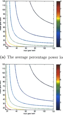
If the model is integrated along the line of action, we obtain the contour plot of the torque loss coefficient as a function of number of teeth on the driving and driven gear shown in Figure 2-2a. The gear module is fixed at 0.5 mod and the sliding friction coefficient p is 0.3, a typical value for dry steel-steel contact.

The model shows that power loss in gears is highly dependent on the size of gears used. For a constant gear ratio which can be represented as a straight line from the origin on the contour plot, the amount of power loss varies with the specific size selection of the gears. In particular, using smaller gears to achieve the same gear ratio results in greater torque loss. This is due to 'relative module' which we define as the tooth size or module compared to the size of gear. If two gear sets have the same size gears but differing modules, the set with larger module would have a longer line of action. The length of the line of action is given by Equation 2.3 where Rs, is the

N

(a) Force diagram of gear teeth before the contact point reaches the centerline

(b) Force diagram of gear teeth after the contact point passes

the centerline

Figure 2-1: Force diagrams of single gear contact between two teeth. The sliding

direction changes as the contact point moves past the centerline and the sliding friction force changes direction

V

3

input gear teeth

(a) The average percentage power loss

CL

8

7

6

(b) Symmetric part of average

percent-age loss

3

I

3

input gear teeth

0.03 0.02 0.01 -.01 -0.02 -0.03

(c) Skew symmetric part of average per-centage loss

Figure 2-2: Results of the single tooth gear friction model averaged over the line of

action for several combinations of input and output gear sizes. All gears are 0.5 mod and 200 pressure angle. The sliding friction coefficient is 0.3.

I I a 7 3 2 2 0

outer radius and Ri,bsee is the base radius of the side i gear. In Equations 2.1 and 2.2, the greater the distance a from the centerline, the greater the torque loss. Therefore average torque loss can be reduced by using larger gears or lower module. This result is consistent with the finer teeth used on lowloss gears compared to standard gears

[6].

Length of

- Rbase + RS - Rbase, -

(R

+ R

)sin(a)

(2.3)

line of action

To better study the asymmetry in power loss in a single gear set for the two power transfer directions, the average power loss can be separated into symmetric and skew components. The values of symmetric and skew loss are calculated using Equations 2.4. The symmetric contour plot shows the average loss between the two driving cases for the same two gears. The skew component shows the deviation from the average of the two scenarios or the symmetric component. From Figure 2-2c, it is clear that for a given set of gears, there is more loss when the large gear is driving the small one. In normal gearing, the backdriving torque loss is higher, further increasing backdriving impedance compared to the forward driving. The effect is most pronounced at extreme gear ratios and there appears to be minimal difference in loss when the gears are above a certain size (30 teeth).

Symmetric loss(i, j) = _{0.5(Loss(i, j) + Loss(j, i))()}

Skew(i, j) = 0.5(Loss(i, j) - Loss(j,

i))

2.2

Dynamics of Lossy Transmissions

In many cases, geared transmissions are considered without energy loss. The speed reduction and force amplification are derived from the kinematics of the gearing ratio. In this case of perfect energy transmission, the dynamics of a typical system can be

described with a familiar differential equation.

72 D2 J2

Ti -

=

+

ri is the torque applied by the motor, T2 is the torque applied by the load on the

output shaft, D1 is the sum of all damping on the motor shaft, D2 is the damping on

the output shaft, J1 is the inertia on the motor shaft, J2 is the inertia on the output

shaft, N is the gear ratio.

For applications in which backdrivability is important, the backward impedance can be minimized by keeping a low gear ratio, and by reducing the amount of damping and inertia present on the motor shaft.

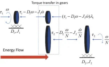
In reality, transmissions must exhibit some degree of power loss from friction in the gears. Thus the expected amount of torque from the output side of the gear set should be slightly lower than what is given by kinematic velocity ratio. If it is assumed that there is some constant power loss, then there will be some asymmetry in the dynamic equations depending on the direction of power transmission. Figure 2-3 shows the dynamics when power is flowing out of the motor and to the load considering the a torque loss factor of A. In the case of kinematically coupled gear transmissions, the power loss factor and torque loss factor are the same. The equations become

(1

-

)r

-

=

((1

-

)D

+

)

+

((1

-

A)J1

+

(2.6)

for power flowing from side 1 to side 2 and

T1 - (1 - A2) = (D1 + (1 - 2) )W + (J1

+

for power flow from the side 2 to side 1.

A,

Torque transfer in gears r

- DI(O -

3

Energy Flow

Figure 2-3: The force diagram of power flow from side 1 to side 2 through a set of gears. Loss is taken as a factor of torque entering the gear mesh that does not become amplified by the gear ratio.

Chapter 3

Gear Friction Experiment

3.1

Experimental Setup

The experiment was conducted with two brushless motors driving the shafts of the

two gears. By controlling the current in each motor, precise torques could be applied

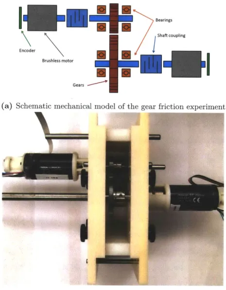
at each shaft. Figure 3-1 shows the complete mechanical design. Depending on the

motor torque and spinning direction, one motor can act as a power source and the

other as a virtual load. Since the two shafts are kinematically coupled by the gear

ratio, a comparison the torques applied at each shaft can determine the amount of

torque and power loss through the mechanical system. The virtual load apparatus

allows the two motors to switch roles and reverse the power transmission direction.

The testing apparatus was designed to accommodate a variety of gear

combina-tions. The two inner plates hold one motor shaft and its driving motor. The two

outer plates hold the second shaft and its driving motor. In each set of plates, dowel

pins are used to maintain the relative alignment of the two plates and bearings. The

two sets of plates can slide relative to each other in order to precisely control the

dis-tance between the gears. Locating pins are mounted on each set of plates so that the

distance between the two drive shafts can be easily measured with calipers. Figures

3-2 and 3-3 show an exploded view and the locating features respectively.

In a typical robotic actuator, the motor shaft uses a smaller gear than the output

shaft to obtain torque amplification. In the forward driving case in which the motor

Encoder

Brushless motor Gears

Bearings Shaft coupling

(a) Schematic mechanical model of the gear friction experiment

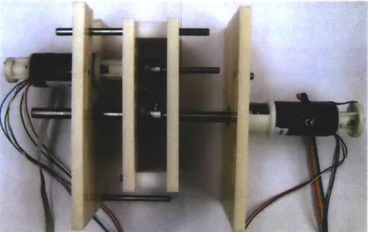
(b) Picture of the mechanical experimental setup

Figure 3-2: Partially disassembled mechanical setup showing the two sets of plates,

each holding a motor and driveshaft.

Figure 3-3: The distance between locating pins on each set of plates is used to precisely

power flows to some load at the output shaft, the motor on the small gear side applies

torque in the direction of movement to do positive work. The motor on the large gear

side does negative work by applying torque in the direction opposite of travel. In

the backdriving case in which the energy flows from the load side into the motor, the

motor on the shaft of the larger gear applies torque in the direction of travel and the

motor on the small gear side applies torque in the opposite manner.

3.1.1

Motor Driver

For the experiment, sinusoidally commutated ironless brushless motors were used as

the torque source in order to provide smooth torque profile. Unlike brushed DC

mo-tors, which experience torque ripple over the course of rotation due to the discrete

contacts in the commutator, electrically commutated brushless motors can

continu-ously change the direction of the magnetic field in the stator as the permanent magnets

on the shaft rotate. Additionally we used an ironless motor to avoid potential cogging

torque when the rotor magnets line up with the stator teeth. The particular motor

chosen for the experiment was a Maxon EC32 (Order Number 118888) three-phase

brushless motor. The standard method of commutating the motor uses internal hall

effect sensors is to measure rotor position in relation to the stator. The six different

combinations of outputs dictate which wires should be connected to the positive and

negative rails of the electric supply. This method, known as six-step commutation

or block commutation is the easiest to implement but suffers from the torque ripple

since it mimics the discrete commutation of brushed DC motors [8].

Sinusoidal commutation for brushless motors requires much more sophisticated

electronics and controls compared to DC motors. All measurements must be accurate

for proper force production and the challenges in calibration are described in 3.1.2.

For one motor, three National Instruments NI 9505 DC Brushed Servo Drives were

configured so that each driver only formed a half bridge connecting to one of the motor

leads. In series with each motor lead was a LEM CASR-15NP current sensor capable

of sensing bidirectional currents of 15 A. The analog outputs of the current sensor

were read by an NI 9205 16-bit analog input module. Rotor position was sensed by a

RLS RMB20SC13BC1O 13-bit digital magnetic encoder that sensed the position of an

accompanying magnet attached to the shaft of the motor. The setup was duplicated

for the second motor and all National instruments modules were mounted in a NI

cRIO-9082 chassis. The control electronics are shown in Figure 3-4.

Figure 3-4: National Instruments NI cRIO-9082 chassis showing the control

electron-ics. From left to right, the first three and last three slots house N19505 DC Brushed

Servo Drive used to drive a single phase of a three-phase brushless motor. A LEM

CASR 15-NP hall effect current sensor is mounted above each motor driver and

mea-sures the current in that phase. The fourth slot is a NI 9205 analog input module used

to measure the output of the current sensors. Slot 5 is a direct digital connection to

the two magnetic encoders on the motor shafts.

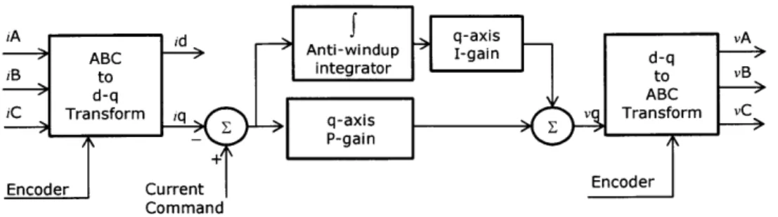
The technique employed by the custom motor driver is field oriented control.

During each step of the control loop, the rotor position and the three phase currents

are measured and new phase voltages are issued. Using the DQO transformation, the

Q-axis current corresponding to the torque producing current is calculated. A PI

controller on

Q

current is then used to issue the next

Q

voltage command in order to

regulate motor current to the set point. The

Q

voltage command is then transformed

by the inverse DQO transformation to calculate new phase voltages. These voltages

are then produced by the NI 9505 drivers using PWM at 20 kHz. Feedback control

occurs every cycle of the PWM output. The entire algorithm was implemented on

the integrated FPGA in the NI cRIO-9082 using LabVIEW. Figure 3-5 shows the

architecture of the current controller.

Figure 3-5: The block diagram of the control algorithm used in to drive the brushless

motors

3.1.2

Motor Calibration

The two motors used for the drive source and load were calibrated to find the torque constant. The torque constant in the specification are for six step commutation and are not valid for the sinusoidal commutation used for the experiment. To find the motor constant, the motor shaft was externally driven at constant velocity and the relative voltages between the three phases were captured by oscilloscope. The motor

velocity w was estimated from the period of the phase voltage sinusoids and the motor constant k was computed by the equations in 3.1 for back EMF of each phase. To

find the torque constant using sinusoidal commutation, the torque for each phase of the motor winding is summed and given by Equation 3.2 in which T is the motor torque and Iq is the torque producing quadrature current calculated from the DQO transformation of the three phase currents.

SVA

VB

Wkcos(O

(3-1)

Uc = wkcos(O

+

r

1.5kI1

(3.2)

In order for the motor torque to match the calculated motor constant, the shaft

position must be correctly calibrated to send the correct sinusoidal currents at each position. This procedure is conducted by removing all loads from the motor and

sending a constant current to the motor and recording the rest position of the rotor. The offset to obtain the torque calculated from the oscilloscope measurement is 90 electrical degrees so the sinusoidal pattern is advanced by 90 degrees to obtain the correct phase currents for the recorded position.

In addition to calibrating for shaft position , the current sensing in each phase of the motor must be accurate. Early experiments using low cost hall-effect current sensors suggested erroneously, that the gears were more than 100% efficient due to the sensitivity of the sensors being off by up to 7% from the stated specifications. Another issue with current sensors was drift which caused the zero current output voltage to shift over time. To ensure proper measurements, the sensitivity was verified with several test currents and each current sensor was zeroed periodically throughout the experiment.

3.2

Experimental Method

In the experiment, a set of gears were tested at a constant gear pitch line velocity of 500 teeth/s. The power transmitted through the gears was increased by gradually increasing the resistance torque of motor doing negative work. A PID controller on velocity was used to find the steady state torque on the driving motor to maintain the constant velocity. At constant velocity, the transmission dynamics from equations 2.6 and 2.7 simplify to

(1 - )r1- - = ((1 A)Di + )W (3.3)

N+

for energy flow from side 1 to 2 and

71 - (1 - A2) N = (D1 + (1-A2) ) (3.4)

for energy flow from side 2 to 1. The torque lost through the gear mesh can be easily calculated from the slope of the output vs input torque line at constant velocity.

3.3

Results

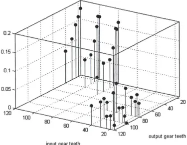
Several combinations of gears were tested to find the dependence of power loss on gear size selection. All gears tested gears were 0.5 mod metric gears manufactured by Stock Drive Products/Sterling Instrument to ISO Class 7 standards. The material was 303 stainless steel and the gears were run dry. Pinion gears ranging from the 16 teeth to 40 teeth were paired with larger gears of 80, 100 and 120 teeth. During the experiment, the motor on driving gear side was used to provide positive work while the motor on the other shaft provided a load resistance. The relationship of drive torque and load torque was fit by linear least squares to obtain the slope and the loss was calculated using Equation 3.3. The loss factor of all drive combinations are shown in Table 3.1. The data are plotted in Figure 3-6.

0.2--0. 15 -0.1 -0. --- - - 4 120 1-100 6 80 80 60 40 100

20 120 output gear teeth

input gear teeth

Figure 3-6: Loss factors of different gear pairs obtained from experiment.

3.4

A new loss model

The data has the same tendencies as the single tooth friction model in Section 2.1. However, it matches much more closely with the skew symmetric plot of loss than the total loss in Figure 2-2. In order to correct the model, we calculate the symmetric

and skew components of the data using Equation 2.4 and use them to rescale the

symmetric and skew components of loss in the single tooth model.

The magnitude of the skew behavior is many times that of the theoretical model.

Whereas the model predicted that the maximum component of total loss due to

asymmetric loss was 0.015%, the experiment showed close to 10%. In Figure 3-7, the

skew data is shown with the theoretical skew using a sliding friction coefficient of

0.5. The large friction is consistent with unhardened stainless steel to stainless steel

sliding contact when the surfaces are curved in Hertzian contact as in the curved gear

tooth profiles [3]. In addition, a scaling factor of 100 is applied to the theoretical

model. The data matches closely with the new corrected model.

0.1

o.15,

0.06

output gear teeth input gear teeth

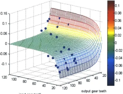
Figure 3-7: The skew data plotted with the scaled theoretical model using friction

coefficient u=0.5 and scaling the model by a factor of 100. The blue points are the skew

components of the experimental data and the surface plot is the corrected model.

Whereas the model in Section 2.1 showed a dominant symmetric component of

friction, symmetric component of the data has closer magnitude to the skew. Using

the 0.5 friction coefficient that is used to fit the skew, the symmetric loss data fits

the model without a scaling factor as shown in Figure 3-8. A constant term of 0.025

is added for to compensate for the steady state loss independent from gear selection.

This loss is most likely caused by coulomb friction in the bearings which was not

considered in the single tooth model. The data confirms that regardless of power

transfer direction, the average loss in a gear set is reduced for larger gears.

o.13 0.150 0.11 0.1 0.09 0.05 --.- 0.08 0.07 0 20 -- - -- - -- 20 0.06 40 -- -4 . 0 60 -. - - -- 60 so -s-o8 0.05 100 100

output gear teeth 120 120 input gear teeth

Figure 3-8: The symmetric data plotted with the theoretical model using friction

coefficient u=0.5 and adding a steady state component of 0.025. The blue points are

the symmetric components of the experimental data and the surface plot is the corrected

model.

3.4.1

Direction Impedance

The data clearly shows that the asymmetry of gear loss over power transfer direction

in a single set of gears. In addition, the data confirms that power loss in a set of gears

is always greater when the larger gear is driving the smaller one. The difference in

power loss is up to 17% in the pair of gears with largest difference in size (16, 120).

The asymmetry is reduced sharply as the 16 tooth gear is increased. With a 30 to

120 tooth combination, the difference in power loss is 4%. When both gears exceed

35 teeth, the magnitude of skew loss is 1%, equivalent to 2% in actual difference

between the two power transfer directions. These results show that directional loss

can be greatly minimized by selecting larger pinions. The tradeoff is between the

impedance of larger gear inertia and directional loss.

expected from the simple single tooth model. While the trends are the same, the single tooth contact assumption is inadequate for accuracy. It is possible that the discrete contact of the second tooth may amplify the normal forces on the sliding surfaces or that other unmodeled behavior acts in the same manner as the single tooth friction model but with a larger magnitude.

Table 3.1: Power loss values for several combinations of driving and driven gears.

Driving gear teeth Driven gear teeth loss factor A

16 80 0.037 16 100 0.001 16 120 0.013 18 80 0.059 18 100 0.019 18 120 0.024 20 80 0.040 20 100 0.041 20 120 0.036 24 80 0.049 24 100 0.038 24 120 0.032 30 80 0.070 30 100 0.075 30 120 0.068 40 80 0.078 80 16 0.163 80 18 0.150 80 20 0.147 80 24 0.102 80 30 0.078 80 40 0.075 100 16 0.167 100 18 0.144 100 20 0.170 100 24 0.109 100 30 0.077 120 16 0.179 120 18 0.159 120 24 0.142 120 30 0.109

Chapter 4

Conclusion

4.1

Actuator Modeling

The work on geared transmission dynamics presented in this thesis is useful for appli-cations involving the control of geared systems. The results are particularly necessary for modeling dynamics of robotic systems in which the motor does both positive and negative work during acceleration and braking respectively. In these cases, the differ-ent amounts of friction loss should be incorporated into the dynamics. In experimdiffer-ent, the power loss values could differ by up to 17%. In applications such as automobiles in which the engine only acts mostly as a power source, the gear loss results can be applicable to accurately model the amount of torque that is transmitted to the wheels for the many gear combinations in the gearbox.

4.2

Actuator Design

The gear friction results presented in this paper can inform new actuator designs. The experimental data clearly showed the asymmetry of power loss depending on the power transfer direction. In running robots where backdrivability is necessary for proper energy exchange with the ground, the motor and geared transmission can be chosen to minimize the impedance while still achieving proper output torques. The results clearly show that larger gears can reduce overall friction loss, and gears more

closely matched size can reduce the amount of added friction loss in the backdriving direction when energy flows into the motor. In hybrid electric vehicles that rely on regenerative braking, the efficiency for both directions of power flow can be optimized.

4.3

Future Work

The model presented in this paper makes simplifications about interaction between two gears. A more detailed model may be able account for the errors in the single tooth contact model. In the experiment, gears were run dry to easily maintain the same conditions over multiple experiments. However in application, gears are always used with lubrication and future work would examine the effects of lubricant to model more realistic operating conditions.

Bibliography

[1] NE Anderson and SH Loewenthal. Comparison of spur gear efficiency prediction

methods. 1983.

[2] H. Asada and K. Youcef-Toumi. Shigley's Mechanical Engineering Design (Mcgraw-Hill Series in Mechanical Engineering). McGraw-Hill

Science/Engi-neering/Math, 1986.

[3] DH Buckley. Friction behavior of 304 stainless steel of varying hardness

lubri-cated with benzene and some benzyl structures. (September), 1974.

[4] Richard Budynas and Keith J. Nisbett. Shigley's Mechanical Engineering Design

(Mcgraw-Hill Series in Mechanical Engineering). McGraw-Hill

Science/Engi-neering/Math, 8 edition, October 2006.

[5] M.E. Dohring, E. Lee, and W.S. Newman. A load-dependent transmission

fric-tion model: theory and experiments. In Robotics and Automafric-tion, 1993.

Pro-ceedings., 1993 IEEE International Conference on, pages 430 -436 vol.3, may

1993.

[6] BR H6hn, Klaus Michaelis, and M HinterstoiB er. Optimization of gearbox

efficiency. Goriva i maziva, pages 462-480, 2009.

[7] Y. Michlin and V. Myunster. Determination of power losses in gear transmissions

with rolling and sliding friction incorporated. Mechanism and Machine Theory,

37(2):167-174, February 2002.

[8] Maxon Motor, May 2012. Sales catalog.

[9] Chanat Ratanasumawong, Puwadon Asawapichayachot, Surin Phongsupasamit,

Haruo Houjoh, and Shigeki Matsumura. Estimation of Sliding Loss in a Parallel-Axis Gear Pair. Journal of Advanced Mechanical Design, Systems, and

Manu-facturing, 6(1):88-103, 2012.

[10] Sangok Seok, Albert Wang, David Otten, and Sangbae Kim. Actuator Design

for High Force Proprioceptive Control in Fast Legged Locomotion.

[11] E.C. Wu, J.C. Hwang, and J.T. Chladek. Fault-tolerant joint development for

the Space Shuttle remote manipulator system: analysis and experiment. IEEE