PATRICK P. ERK
B.S., Technische Universitdit Berlin, West Germany
(1987)
Submitted to the Department of
Aeronautics and Astronautics
in Partial Fulfillment of the Requirements
for the Degree of
Master of Science
in Aeronautics and Astronautics
at the
Massachusetts Institute of Technology
September 1990
© Patrick P. Erk 1990
The author hereby grants to M.I.T. permission to reproduce and
to distribute copies of this thesis document in whole or in part.
Signature of
Author-Department of Aeronautics and Astronautics
September 28, 1990
/
C. Forbes Dewey, Jr.
Profes on of Mechanical Engineering
Thesis Supervisor
Accepted by
..
MASSACHUSEfTfS INSTITLWlEOF
rEC~on.oEY
SEP 19
1990
LIBRARIESV
Professor Harold Y Wachman
Chairman, Departmental Graduate Committee
I
Certified by
__ ___ , , , , , , , ,_
F
Submitted to the Department of Aeronautics and Astronautics
on September 28, 1990 in Partial Fulfillment
of the Requirements for the Degree of
Master of Science in Aeronautics and Astronautics
Abstract
Digital signal processing algorithms in laser-Doppler anemometry still lag behind the
standards used in Doppler-radar or sonar technology. The two main problems in
laser-Doppler signal processing are signal detection and frequency estimation. In this Thesis, a
software system for use in flow experiments with laser-Doppler anemometry has been
developed. It features programs for digital prefiltering, for FIR filter design, for burst
detection, and for frequency estimation. Spectral estimation is done with an algorithm
based on the discrete Fourier transform or with an auto-regressive moving-average
algo-rithm based on a Pade approximation to the signal spectrum. The Modified Covariance
Algorithm and the Iterative Filtering Algorithm have also been tested on synthetically
generated Doppler signals. Flow experiments with a cone-and-plate flow show the
wor-kability of the software system. These results also confirm the validity of the assumptions
made in the numerical simulations.
Thesis Supervisor: C. Forbes Dewey, Jr., PhD
Title: Professor of Mechanical Engineering
_II·_·I _·~II~_1~~_L~_
_ ~~·_
_____I
I-·C-lll- .11_4~---·-~11~·-1~
I would like to thank ...
... Prof. Dewey for this great learning opportunity and his support
Donna for teaching me what the US is all about and who is in the end
responsible for this mess
... Natacha for Tacos, housing opportunity in NYC, and a gorgeous flow
apparatus
Bob and Andrew for many, many walks to the local coffee supply,
among other things
... Jason for doing most of the work with the laser, asking millions of
ques-tions, and a ride on his roller blades
... Hannes for storing my furniture in Berlin for two years and not selling it
to my now free but still deprived eastern homeboys
My family for their suggestions and comments in all questions of life
... Isabella for giving me such a hard time (sigh)
... And my friends for giving me such a good time
11.1
The Probe Volume
...
13
II.2
The Scattering Process
.
.
.
.
.
.
.
.
.
.
.
.
.
.
.
.
.
.
.
17
II.3
Fluorescent Particles .
.
.
.
.
.
.
.
.
.
.
.
.
.
.
.
.
.
.
.
18
II.4
Computing the Probe Volume Size .
.
.
.
.
.
.
.
.
.
.
.
.
.
.
.
19
III. Digital Spectral Estimation: Survey of Methods .
.
.
.
.
.
.
.
.
.
.
.
.
.
24
IV. Classical Methods of Spectral Estimation .
.
.
.
.
.
.
.
.
.
.
.
.
.
.
.
29
IV.1
Properties of the Discrete Fourier Transform .
.
.
.
.
.
.
.
.
.
.
.
.
30
IV.2 Periodogram: The Nuttall-Cramer Method
.
.
.
.
.
.
.
.
.
.
.
.
.
33
IV.3
Spectrograms ...
36
V. Adaptive Spectral Estimation
.
.
.
.
.
.
.
.
.
.
.
.
.
.
.
.
.
.
.
37
V.1
General Introduction ...
38
V.2
Autoregressive Spectral Estimation
.
.
.
.
.
.
.
.
.
.
.
.
.
.
.
39
V.3
Algorithms for AR Spectral Estimation
.
.
.
.
.
.
.
.
.
.
.
.
.
.
42
V.4
The Iterative Filtering Algorithm
.
.
.
.
.
.
.
.
.
.
.
.
.
.
.
.
46
V.5
Autoregressive-Moving Average Spectral Estimation .
.
.
.
.
.
.
.
.
.
48
VI. Preliminary Processing of LDA Signals
.
.
.
... . .
.
.
.
.
.
.
.
..
.
.
55
VI.1
Digital Filtering with the Overlap-Add Method .
.
.
.
.
.
.
.
.
.
.
.
56
VI.2
Design of Finite-Impulse Response (FIR) Filters
.
.
.
.
.
.
.
.
.
.
.
58
VI.3
Corrections for Velocity Gradients and Velocity Fluctuations .
.
.
.
.
.
.
.
59
VII. Numerical Simulations with the MATLAB Software Package .
.
.
.
.
.
.
.
.
.
64
VII.1 Signal Generation .
.
.
.
.
.
.
.
.
.
.
.
.
.
.
.
.
.
.
.
.
64
VII.2 Testing of the Algorithms Using the MATLAB software
.
.
.
.
.
.
.
.
.
67
VIII. A Software System for Processing LDA Signals .
.
.
.
.
.
.
.
.
.
.
.
.
.
73
VIII.1 Available Computational Resources
.
.
.
.
.
.
.
.
.
.
.
.
.
.
.
73
VIII.2 Descriptions of the Programs
.
.
.
.
.
.
. .
.
.
.
.
.
.
.
.
.
74
VI.3 Caveats of the Programs and Some Hardware Recommendations
.
.
.
.
.
.
83
IX. Application of Software System for LDA to Cone-and-Plate Flow
.
.
.
.
.
.
.
.
86
IX.1
The Cone-and-Plate Flow
.
.
.
.
.
.
.
.
.
.
.
.
.
.
.
.
.
.
86
IX.2 Experimental Design .
.
.
.
.
.
.
.
.
.
.
.
.
.
.
.
.
.
.
.
88
IX.3
Experimental Results .
.
.
.
.
.
.
.
.
.
.
.
.
.
.
.
.
.
.
.
93
X. Conclusions and Direction of Future Work
.
.
.
.
.
.
.
.
.
.
.
.
.
.
.
98
Literature
...
.
...
.
102
Appendix 3.3: Results of the Iterative Filtering Algorithm .
...
117
Appendix 3.4: Results of the Pade Estimator Using the Common Euclidean
Algorithm
.
.
.
.
.
.
.
.
.
.
.
.
.
.
.
.
.
.
.
.
.
.
.
.
118
Appendix 4: Experimental Results .
.
.
.
.
.
.
.
.
.
.
.
.
.
.
.
.
120
Appendix 5: Programs for Processing LDA Signals .
...
121
Appendix5.1: #include file FileOp.h forFile Operations
.
.
.
.
.
.
.
121
Appendix 5.2: SampleData - Program for Data Acquisition .
...
123
Appendix 5.3: FilterData
-
Program for Filtering Input Data with FIR
Filter .
.
.
.
.
.
.
.
.
.
.
.
.
.
.
.
.
.
.
.
.
.
.
.
.
.
129
Appendix 5.4: CreateFIR - Program for FIR Filter Design .
.
.
.
.
.
.
.
136
Appendix 5.5: KaiserFIR
-
Routine for Kaiser Window Design
.
.
...
..
142
Appendix 5.6: Variance
-
Program Computing First Order Statistics of
Signal
...
...
145
Appendix 5.7: GetBursts
-
Program for Burst Validation .
...
....
.
151
Appendix 5.8: MeanSpec
-
Program Computing the Mean Spectrum
.
.
.
.
.
.
159
Appendix 5.8.1: PadeApprox - Initializes polynomials for Euclidean Algorithm 169
Appendix 5.8.2: EucAlgVA
-
Vectorized Euclidean Algorithm 170
Appendix 5.8.3: PolyDivVA - Polynomial Division on the Vector Accelerator 173'
Appendix 5.8.4: ConvolveVA Program for Polynomial Multiplication 174
-Appendix 5.8.5: CheckOrderVA
-
Program for Removing Leading,
Zero Coefficients
175
Appendix 5.8.6: ArmaP sd
-
Program Computing the ARMA Spectrum
176
Appendix 5.9: MeanVel
-
Program Computing the Mean Velocity Profile .
....
178
Appendix 5.10: DoPlot - Plot Program ...
.
.
.
.
.
183
Figure 1. Single-component, fringe-mode laser-Doppler anemometer [from 7]
. ...
12
Figure 2. Effect of several particles crossing the probe volume at the same time [ from 8]
.
. .
14
Figure 3. Misalignment of the beams creates an asymmetric fringe pattern [from 8] ...
15
Figure 4. Intensity distribution due to scattering [from 8] (direction of the incident light indicated
by arrow, particle size decreasing from from (a) to (b))
. . . .
. . . .
. .
17
Figure 5. Signal quality and signal strength depend on the particle size (from [9]) ...
.
. .
18
Figure 6. Optical configuration for LDA in this project ...
. . . .
. .
20
Figure 7. Survey of Digital Spectral Estimation Techniques as applicable to LDA
. . .
. .
25
Figure 8. Spectral Estimation by Parameter Models . ...
26
Figure 9. Low resolution resulting from finite-length data set [from 10] ...
...
....
.
31
Figure 10. Rectangular window: (a) time series, (b) log-magnitude of DFT [from 10] ...
. .
33
Figure 11. Hamming window: (a) time series, (b) log-magnitude of DFT [from 10]
. ..
. .
34
Figure 12. Dolph-Chebyshev window
a
=
2.5: (a) time series, (b) log-magnitude of DFT
[from 10]
...
35
Figure 13. Iterative Filtering Algorithm
.
.
.
.
.
.
.
.
.
.
.
.
.
48
Figure 14. The overlap-add method (from [25]). (a) segmentation of the input data,
(b) each segment is convolved with the filter impulse response and
over-lapped with the following segment .
...
57
Figure 15. More particles with higher velocity will cross the probe volume than
particles with lower velocity ...
....
.
.
.
....
61
Figure 16. System structure .
.
.
.
.
.
...
.
.
..
.
.
.
.
75
Figure 17. Flowchart of the burst validation algorithm .
.
.
.
.
.
.
.
.
78
Figure 18. Flowchart of the Pade spectral estimator .
.
.
.
.
.
.
.
.
.
81
Figure 19. Geometry of the cone-and-plate flow .
.
.
.
.
.
.
.
.
.
.
87
Figure 20. Photo 1 of the experimental set-up: cone-and-plate apparatus with LDA
front lens and mirror. The dial indicator is used to determine when the
apex of the cone hits the glass plate. The support in the middle of the
glass plate prevents bending. .
...
. ..
.
89
Figure 21. Photo 2 of the experimental set-up. From left to right, bottom to top:
oscilloscope, filter, DISA Photomultiplier power supply and counter for
blue light, dito for green light, DISA frequency mixer, laser, LDA
optics.
..
..
...
90
Figure 22. Results from calibration experiments, the gap was filled with 100%
gly-cerine, the angular velocity of the cone was increased from 15 rpm to 41
98
Figure 25. Mean spectrum of two bursts with the Pade estimator.
99
Figure 26. Simulated LDA signal, 20 bursts, SNR
=
2000 dB, seeding meapaus=
0.0001. The high seeding leads to overlapping bursts. This signal is the basis
for all subsequent numerical simulations where only white noise is added to
this signal.
.
.
.
.
.
.
.
.
.
.
.
.
.
.
.
.
.
.
..
112
Figure 27. White noise has been added to the signal of the previous Fig. SNR = 0 dB.
Burst detectors based on some envelope criteria as the one used in this project
will validate only the strongest bursts .
.
.
.
.
.
.
.
.
.
.
.
112
Figure 28. Changes in the local SNR ratio over 128 point long segments overlapping by
50 %. For a constant background noise, the SNR will be lowest for particles
crossing the center of the probe volume (strongest signal)
.
.
.
.
.
.
113
Figure 29. Result of classical spectral estimator: DFT of Hamming windowed (128
points) data. The segments were overlapped 50 %. SNR
=
10 dB same signal
as in Fig. ####. The variance in the spectral estimate is high.
....
.
114
Figure 30. Location of the spectral peaks in the previous Fig. Although the spectral peaks
are hardly recognizable in the spectrogram, they correspond well to the
Doppler frequency of the signal .
.
.
.
.
.
.
.
.
.
.
.
.
.
114
Figure 31. Third order AR model with the 10 dB signal. Note the very low variance in the
spectral estimate. The spectra are of 128 point long segments overlapped by
50 % ....
...
...
...
115
Figure 32. Location of spectral peaks in the previous Fig. The Doppler frequency is well
resolved. The drop-outs correspond to the locations of lowest local
SNR
.
.
.
.
.
.
.
.
.
.
.
.
.
.
.
.
.
.
.
.
.
115
Figure 33. The estimator from the previous two Fig. applied to a 0 dB. The low SNR
results in a decrease of the performance. .
...
.
116
Figure 34. The location of the spectral peaks for the Modified Covariance Algorithm and
a 0 dB LDA signal (previous Fig.) shows that the Doppler frequency is not
resolved very well...
116
Figure 35. A 20th order AR estimate for a 2000 dB signal again with 128-point segments
demonstrates that too high a model order results in spurious peaks in the
spec-trum. The variance in the estimate increases
...
.
117
Figure 36. IFA with a third order AR Modified Covariance Agorithm after 8 iterations.
The SNR of the signal is 0 dB. The spectrogram is very smooth and of very
low variance. ...
...
117
Figure 37. The spectral peaks in the previous Fig. correspond to the Doppler frequqncies.
Figure 40. Generally, if shorter data segments were taken, the performance of the
auto-regressive models decreased. The Pade estimator seemed to be less sensitive in
this case. This Figure shows the performance with 64-point segments
over-lapped by 50
%.
SNR is 10 dB, order of the AR branch is 4. ....
.
.
.
119
Figure 41. In the case of the shorter data segments of the previous Figure the Doppler
fre-quency is still resolved very well. However, more drop-outs occur at low local
SNR.. ...
119
Figure 42. Spectrum of Pade estimator after digital lowpass filtering with
Filter-Data. Comparison with Figs. 24 and 25 shows that the low frequncies are
TABLE 1. Geometry of the probe volume. See Fig. 1 for definition of the
variables .
.
.
.
.
.
.
.
.
.
.
.
.
.
.
.
.
.
.
16
TABLE 2. Properties of Rectangular, Hamming, and Dolph-Chebyshev window
2[10]
.
.
.
.
.
.
.
.
.
.
.
.
.
.
.
.
.
.
.
.
32
TABLE 3. Filter specifications for Butterworth filter
.
.
.
.
.
.
.
.
.
68
TABLE 4. Data set for the numerical simulations
.
.
.
.
.
.
.
.
.
.
69
TABLE
5.
Optical parameters for
Xk
514.5nm, 488nm
.
.
.
.
.
.
.
.
.
91
Laser-Doppler anemometry (LDA) has proven to be an extremely useful
experi-mental tool for measuring fluid flow velocities. Its advantages over the complementary
technique in fluid mechanics, hot-wire anemometry, are the non-intrusive nature of LDA
measurements, the large dynamic range from zero to supersonic speeds, and a versatility
and extendibility to special experimental conditions such as 3-dimensional velocity
measurements and measurement of the different phase velocities in multi-phase flows.
The fundamental principle behind laser-Doppler anemometry is the detection of
the Doppler frequency of light scattered from particles traversing the point of intersection
of two laser beams. This Doppler frequency is directly proportional to the velocity of the
particle. Due to the finite size of the measurement volume, inaccuracies occur in the
pres-ence of velocity gradients or turbulpres-ence. Proper averaging techniques (cf. Section VI)
may reduce the systematic error in the measurements for these cases.
Noise in laser-Doppler anemometry is mainly non-Gaussian [9] and comes from
the photodetector or from scattered light from surfaces or distant particles. The
signal-to-noise ratio can be significantly improved if fluorescent rather than scattering particles
are used [20][34].
Recent publications concentrate on the use of Fourier transform of either the data
or the autocorrelation function of the data [2][9][11][17][18][22][26][31]. Both methods
represent the classic way of doing spectral analysis. New methods of spectral estimation
have been developed over the last ten years [14][19][25]. They are based on fitting the
coefficients of a linear constant coefficient equation (cf. Section V.1) to the data using
some error minimizing criterion (e.g. least squares). These newer algorithms are now
routinely used for detection and analysis of sonar and radar signals [13][14][29]. Their
use in laser-Doppler signal processing is only limited [33]. This Thesis applies some of
these more "advanced" algorithms to laser-Doppler anemometry.
Numerical simulations were carried out in order to assess the performance of the
different algorithms for LDA signals . The "traditional" spectral analysis procedure in
LDA is compared to three other methods: an auto-regressive estimator, the Modified
Covariance Method (cf. Section V.3.4), an enhancement of this algorithm, the Iterative
Filtering Algorithm (cf. Section V.4), and an auto-regressive moving-average estimator
based on the Pade approximation (cf. Section V.5). Then, the most promising method,
the Pade estimator, is tested in a real flow experiment (cone-and-plate flow, cf. Section
IX.1). For these flow experiments, it was necessary to implement a system of programs
for processing LDA signals (i.e. sampling, filtering and digital filter design, burst
valida-tion, spectral estimavalida-tion, averaging, plot of spectrum/velocity).
The present paper is divided into three major parts: the first part explains the
underlying principles of LDA and of the digital signal processing techniques. The second
part describes the numerical simulations, their results, and the software system for the
flow experiments. The third section introduces the cone-and-plate flow and the
experi-mental set-up and discusses the results obtained by the software system. A final
discus-sion and evaluation is then presented.
II. The Laser-Doppler Anemometer
The laser-Doppler anemometer (LDA) is an optical experimental method which
allows the instantaneous, non-intrusive measurement of the velocities within a flow field.
It is based on the interference of two Gaussian laser beams, and on the light scattering
properties of particles within the flow. Generally, the analytical treatment can be kept
quite simple, because all mathematical approximations are of higher accuracy than the
usually noisy signal. Recent improvements in the signal quality involve the use of
fluorescent rather than scattering particles [20][34].
A typical set-up of a one-component, fringe-mode LDA is shown in Fig. 1.
Detector
Laser
Figure 1. Single-component, fringe-mode laser-Doppler anemometer [from 7]
A Gaussian laser beam is split and the resulting two parallel branches are focused at a
formed. Particles crossing that fringe pattern will scatter the light with a frequency which
is directly proportional to the particle velocity (Doppler frequency). This signal is
received by a photodetector and then further processed.
II. The Probe Volume
The volume contained in the -L-intensity contour of the interference field created
by the intersecting laser beams is called the probe volume. It is of ellipsoidal shape and
filled with an equidistant and parallel fringe system.
In order for the system to be applicable, the probe volume must meet the following
two requirements:
The probe volume has to be as small as possible, as the velocities at a point in the
flow field have to be measured; a large probe volume would only give the spatial
average of the velocities around the point of intersection. In addition, a larger
probe volume would increase the probability that more than one particle crosses
the fringe pattern at the same time. This would result in a random superposition of
Doppler frequencies, reducing the signal quality in the case of destructive
interfer-ence of the two signals (cf. Fig. 2). In practice, the signal processing procedures
and optics impose a lower limit on the number of fringes and on the size of the
probe volume.
* The fringe pattern has to be symmetric, so that particles traversing the probe
volume at different locations cross fringes with the same distance. If this is not the
case, the measured velocity will depend on the crossing path of the particles.
The system is maximized with respect to both items if the waists of the focused
laser beams coincide with the point of intersection.
AB
C
D AA
8
A,B: signals
are
A
c
C,D: signals are
out of
phase
D
If there is more than 1 particle present in the measuring control
volume, constructive or destructive superpositions of signals can
occur.
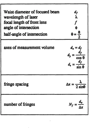
Figure 2. Effect of several particles crossing the probe volume at the same time [ from 8]
Misalignment of the laser beams may result in an elongated and diverging fringe
pattern (cf. Fig. 3) and the probe volume will not be the smallest possible one. If the
waist of the focused beam, wf, lies within the probe volume the formulas of Table 1
describing the geometry of the probe volume apply. For computing wf and the angle of
intersection, ý, see Section II.4 below.
Usually, these effects can be neglected except for large distances between lens and
probe volume. The geometry of the probe volume depends on the angle of intersection, 0:
If 0 increases, the length of the ellipsoid, d,, its height, dy, the fringe spacing, Ax, and the
number of fringes, N, will decrease.
Figure 3. Misalignment of the beams creates an asymmetric fringe pattern [from 8]
The system will detect only the velocity component perpendicular to the fringes.
Oblique passing with the same absolute velocity results in a corresponding decrease of
the Doppler frequency.
The analytical description of the time behavior of the Doppler signal is:
s(t)=
so{ 1+
Ssin
Cos 21 (U t +r,o
(II.1)
r : radius of the particle
Ax: fringe spacing
re.o: location of center of particle at time t=O
Uo: velocity component perpendicular to fringes
so: scaling factor for intensity
Uo
The Doppler frequency is immediately recognized in the argument of the sine as
-AXx
TABLE 1. Geometry of the probe volume. See Fig. 1 for definition of the variables
* Light from particles not crossing the fringe pattern may hit the photodetector. This
effect is taken care of by pinholes in front of the photomultipliers which limit the
depth of the optical field.
* Noise generated in the photoelectric cells stems either from the random emission
of photons (shot noise, Poisson character), from the random movements of
elec-trons (Johnson noise), and from thermal excitation of elecelec-trons. All three types of
noise are broad band and signal-independent. The shot noise depends on the mean
photocurrent: The higher the mean photocurrent the higher the random fluctuations
the higher the shot noise.
Waist diameter of focused beam
df
wavelength of laser
X
focal length of front lens
f
angle of intersection
0
half-angle of intersection
0=
axes of measurement volume
d. = d/
d_cos 0
sin e
fringe spacing
Ax =
11.2 The Scattering Process
The expressions up to now relate only the Doppler frequency to the particle
velo-city. Statements about the field distribution of the scattered light are necessary to
optim-ize signal detection. Analytical results exist only for the case of spherical and ellipsoidal
particles (Mie's Scattering).
Figure 4. Intensity distribution due to scattering [from 8] (direction of the incident light
indicated by arrow, particle size decreasing from from (a) to (b))
The most important result is the non-uniformity of the intensity distribution of the
scattered light (cf. Fig. 4). The intensity of the scattered light will be highest in the
direc-tion away from the focusing optics. This is exploited in the forward-scatter LDA (cf. Fig.
1). The backscatter mode (cf. Fig. 20), the type used in this project, results in a more
compact design but suffers from less intense scattering. Thus, in the backscatter mode, a
smaller signal-to-noise ratio can be expected.
The size of the particles has to be matched to the geometry of the probe volume.
Particles which are too large will cross more than one fringe at a time, but will scatter
more light; particles which are too small produce very weak signals (Fig. 5). It is
recom-mended that the particle diameter is a fourth of the fringe distance [9].
S 6.6 t. : disti
A
Figure 5. Signal quality and signal strength depend on the particle size (from [9])
11.3 Fluorescent Particles
The signal-to-noise ratio in the backscatter mode can be greatly improved if
fluorescent particles are used. Fluorescent particles absorb the incident light and emit
radiation at a longer wavelength. In contrast to the scattering process fluorescent
radia-tion is emitted in all direcradia-tions.
The different wavelength of the fluorescent light allows the use of optical filters to
block all other wavelengths. These filters will reduce the total amount of light at the
pho-tomultiplier and therefore decrease the amount of shot noise in the signal as the mean
photocurrent is reduced.
.. _ _ .__·_.__
_ __. ··
g ntensity
11.4 Computing the Probe Volume Size
The most efficient way to compute the propagation of laser beams is done with ray
transfer matrices (cf. [16]). Each optical element has a particular 2x2 transfer matrix. The
transfer matrix of a system of optical components is simply the product of the transfer
matrices of the single components. Although developed originally for the study of the
propagation of paraxial rays, it can also describe the propagation of laser beams without
changing the matrices for the different optical building blocks.
A paraxial ray is characterized by its distance x from the optical axis (the
z
-axis)
and by the angle 0 with respect to this axis. For paraxial rays, 0 will be small enough to
allow the approximations sin 0
=
0 and cos 0 = 1.
If we define a ray vector, r, by r-
[],
the ray vector behind an optical arrangement,
r, is obtained by multiplying r from the right to the system ray transfer matrix, X:
r =X r.
The optical system used in this project is depicted in Fig. 6. The paraxial laser
beams are focused by a front lens, propagate through a glass plate, and intersect in a
medium of different refractive index. The laser beams are not complanar with the optical
axis. The ray transfer matrices for the different stages are:
Detail of point of intersection
(Probe volume) :
Position of the two
intersecting laser beams
Figure 6. Optical configuration for LDA in this project
X
1=
i
X f 1
(II.2)
For the translation between lens and first surface of the glass plate (index of
refrac-tion =1, distance dl):
~__
. __
dz
1
di
For the refractions at the air-glass and the glass-fluid interfaces, the ray transfer
matrices will be unity (Snell's law). Thus, they do not contribute to the overall system
matrix and can be omitted.
For the propagation within the glass (thickness
d2,
index of refraction n,):
1-X
3
=
0
1
(11.4)
For the propagation of the laser beams through the fluid (index of refraction n
2) to
the point of intersection (distance d3 from the wall):
X
4
=
0
1
(11.5)
The resulting system matrix is:
dz
d
3nt
n2
d2
d
31-
d
+-
+
X = X4 X3 X2 XI = CD=
_1
(11.6)
fi
- -
1
r4=
X r
1.
This yields two equations for the two unknowns
d,
and 0':
dl =f
d
(II.7a)
'= -
(II.7b)
li
The half angle of intersection is found from geometry:
sinO = sine'
(118)
-42
A laser beam of wavelength X and waist diameter
w
0
propagating along the x-axis
has a -- intensity envelope given by:
e
w(z)=wo
1 +
[
]
"
(11.9)
and a curvature of the wave front
R(z)=z [1+
[]2
(11.10)
Defining
a
complex
propagation
parameter
at
a
location
z
1,
__
_
2q(z
1)
=R (z) - j
2
or, equivalently, q (z) = z + j
, the beam diameter and the
field curvature at a position
z
2behind an optical system can be obtained with the complex
propagation parameter at this location and the system's transfer matrix via:
A q(zl)+B
q(z9=
C q(zl)+D
(II.11)
This approach will be used in Section IX.2.1, where we calculate the approximate
geometry of the probe volume.
III. Digital Spectral Estimation: Survey of Methods
In the previous chapter we defined the basic problem of measuring the flow
velo-city as a problem of detecting the burst and estimating the Doppler frequency of a
sinusoidal signal in non-Gaussian noise. Estimation of the frequency content (i.e. spectral
analysis) from sampled data is a problem occurring in many fields of research.
There-fore, a variety of algorithms suitable for implementation on a general purpose computer
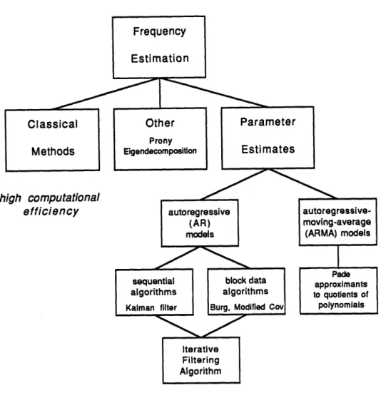
has been developed. Fig. 7 presents an overview which is by no means exhaustive.
We can roughly divide the available spectral analysis techniques into three
categories: classical methods, methods based on parameter estimation, and other
methods.
Classical methods are primarily characterized by their robustness at low SNRs and
their computational speed. They comprise the periodograms, where the data record is
segmented, each segment is then multiplied with a time-window function. Then the
power spectral density (PSD) is estimated by averaging the Fourier-transformed data
seg-ments. The unmatched speed of the classical spectral estimators results from the use of
the fast Fourier transform algorithm (FFT) for evaluating the discrete-time Fourier
transform.
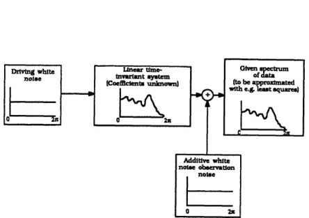
Spectral estimators based on parameter models assume that the
-
unknown
-
spec-trum of the observed data stems from filtering a driving white noise process with a linear
time-invariant system (filter) (cf. Fig. 8). Their basic feature is a very high spectral
reso-lution which enables for example the detection of closely spaced sinusoids. If the data
contain additive white noise (so-called observation noise), the whole process is
h
high spectral resolution
Figure 7. Survey of Digital Spectral Estimation Techniques as applicable to LDA
approximately modeled by a white-noise source whose output is added to the system
out-put.
The underlying assumption of a linear-time invariant filter yields linear
constant-coefficient difference equations for the unknown filter constant-coefficients. These may be solved
by minimizing for example the mean square error between the actual data and the data
Figure 8. Spectral Estimation by Parameter Models
one would obtain by the filtering process.
Although most real processes do not follow these linear difference equations, i.e.
are non-linear, the methods are widely used with good results in many fields [14][16].
As this approach generally requires the data to have zero mean, high-pass filtering
the data before their evaluation is indispensable. This, however, is of no major concern in
LDA, as this kind of filtering is advisable for removing the signal pedestal and the dc
component.
According to the filter type adapted to the data we distinguish between
autoregres-sive (AR) models where the frequency response of the filter driven by white noise has
only poles, and autoregressive moving-average (ARMA), where the filter possesses both
zeros and poles.
The AR estimation techniques now can be subdivided into block data algorithms
and sequential data algorithms [14][19]. Sequential data algorithms update the filter
coefficients each time a new datum comes in. As each update requires a certain number
of operations, these methods cannot be applied in steady-state sense with the data
acquisition. The time required for the update exceeds
-
at least at the sampling
frequen-cies typical for LDA (500 kHz to a few MHz
-
by far the time between incoming data.
Block data algorithms, on the other hand, take one batch of data at a time and process it.
Their performance is slightly superior to that of sequential data algorithms [14][19].
Also, many data acquisition systems, including the one of the computer system used in
this project, operate with buffer queues: they fill one buffer in the memory with the
sam-pled data; when the buffer is full it is released to the operating system; then the next
buffer waiting in the queue is fetched and so on. A processed buffer is put back in the
queue. Thus, block data algorithm seem to be a more natural way to handle spectral
esti-mation.
A widely-used sequential data algorithm is the Kalman filter. Two examples for
ARMA methods are the Modified Covariance Method
-
explained in some detail further
below
-
and the Burg method. Both are very similar, but the former method has
-
at the
same order of computational complexity
-
more favorable features [14].
ARMA methods are mathematically somewhat more complicated. The resulting
least-squares equations are non-linear and cannot be solved efficiently. Certain
assump-tions, however, lead to linearized forms. ARMA models have the advantage of being
able to model noisy processes which are characterized by zeroes in the spectrum.
The method we tested is based the approximation of a high-order polynomial by a
quotient of two (finite) polynomials, termed Pade approximation. At the core of this
algorithm lies the Euclidean algorithm.
The other methods, the best known is probably Prony's method
-
do not really
pro-duce results of higher quality than the preceding two classes. Also, as their computational
complexity is not superior to the parameter estimation techniques, they are not
con-sidered in the remainder of this paper. The Pisharenko Harmonic Decomposition for
instance is based on the eigenvalues and eigenvectors of the autocorrelation matrix.
Further information about parameter models in spectral estimation may be found in
[14][19].
The Iterative Filtering Algorithm finally is a technique which enhances the results
of the AR spectral estimators, which usually perform poorly in the presence of noise
[12][13][14].
IV. Classical Methods of Spectral Estimation
All Classical Methods are based on the computation of the discrete Fourier
transform (DFT) either directly (DFT of the data) or indirectly (DFT of the
autocorrela-tion funcautocorrela-tion). In both cases the properties of the DFT are of importance, the are outlined
in the first section of this chapter.
For the two situations in LDA, scarcely seeded flow and discontinuous signals
(burst-type LDA), and densely seeded flows and continuous signal, we have to use
dif-ferent methods for correctly computing the mean Doppler frequency.
The proper averaging strategy for the burst-type LDA, a method termed
residence-time weighting will be introduced in Section VI.3.
In the case of densely seeded flows, we may apply a simple arithmetic averaging
strategy. Therefore the correlogram and periodogram become valid signal processing
algorithms. The computationally most efficient periodogram method is termed the
Nuttall-Cramer method and is explained below.
If we are more interested in the velocity fluctuations than in the mean we can
present the data in the form of a spectrogram, the way all results of the numerical
simula-tions in Section VII are depicted. In a spectrogram the variation of the spectrum with
respect to time is shown.
IV.1 Properties of the Discrete Fourier Transform
The resolution of all classical spectral estimators using the DFT depends on the
length of the data set
x[n]:
For a data set of length N, sampled with an effective
1
sam-pling frequency of f,, frequencies spaced less than -
cannot be resolved (cf. Fig. 9).
Also, zero-padding of the data
-
i.e. lengthening the data record by adding zeros
-
does
not increase the resolution. The only way to accomplish higher resolution is to include
more data points.
The power spectral density (PSD) of a data set
x
[n] which tells us how the energy
is distributed over the frequency bands is the modulus squared of the DFT:
1 -1
j -2Ck
P. (f)
U
=
I
x[n]e N 12(IV.1)
k
f = -f,, k =0, 1,.-,N-1
f,:
Sampling frequency
x [n ]
=
x
[n
] w [n ]: windowed time series
w [n ]: time-window function (e.g. rectangular window: w [n ] = 1,0 5n < N-1, w [n] =0)
The DFT in Eq. (IV.1) can be evaluated most efficiently by an FFT algorithm which
gives rise to the unmatched speed of these methods.
1. the reason I mention an effective sampling frequency is because we can change the sampling rate with a
discrete-time process: Downsampling (and preceding lowpass filtering) reduces the sampling
frequency, upsampling (with successive highpass filtering) increases the sampling frequency.
Local Minimrna I I V I I I I I a I, I a, r jI I
NM Raevb Pubks RoV be Pb s
Figure
9.
Low resolution resulting from finite-length data set [from 10]
The following argument illustrates the limited resolution of the DFT: If we
win-dow an infinite-length data set
x.[n]
with a time-window function w [n] which is zero for
all n
<0
and
n
2N:
+_.2r• .2f.kn
_21n IN-,I2
Sx[n] w
[n]e
N-
x,[n
]
w[n]e
,
(IV.2)
then this multiplication in the time domain corresponds to a convolution in the frequency
domain. We can rewrite the product in the previous expression:
x
[n ]w
[n ]--> X[k]* W[k]
If the length of the time window increases, i.e. N
-co,
it
follows that
W[k]
- 8[k], the
original spectrum of our data, as x [k]
*
8[k]. X [k].
For a finite window length however, W[k] will be some function depending on the
detailed form of w[n], and will smear the spectrum in the convolution process shown in
Fig. 9. As we decrease the distance between two frequency peaks we eventually reach a
point where the two peaks are smeared into one single peak and we have come to the
limit of our resolution. This whole phenomenon is called spectral leakage.
Highest
Main Lobe
3-dB
6-dB
Window
Side-lobe
Bandwidth
Bandwidth
Bandwidth
Level (dB)
(Bins)
(Bins)
(Bins)
Rectangular
-13
1.00
0.89
1.21
Hamming
-43
1.36
1.30
1.81
Dolph-Chebyshev
-50
1.39
1.33
1.85
(a
= 2.5)
Equation of Window for 0 < n s N-1
Rectangular
Hamming
Dolph-Chebyshev
s•k
cos Ncos-'
[
cosJ
w[n] = 1
w [n] = 0.54 - 0.46 cos
W[k] = (-1)
N
cosh
IN
cosh-I
'
S= cosh
-
-cosh-aTABLE 2. Properties of Rectangular, Hamming, and Dolph-Chebyshev window
2[10]
The choice of the window can be important, as the width of the main lobe
influences the resolution and the height of the side lobes control partly the variance in the
estimate. Three windows
-
Rectangular, Hamming, and Dolph-Chebyshev
-
are presented
in Figs. 10, 11, 12, their properties are listed in Table 2. The rectangular window
possesses the narrowest main lobe and the highest side lobes of all windows. The
Hamming and the Dolph-Chebyshev window have somewhat broader main lobes and
considerably smaller side lobes. They are mostly recommended because they optimize
both quantities.
T
117
I I
tl1'I .1 -10 -! 0 10 (0) 1.25 1.00II
sI
1• is1!
If'
* ! I I I i I ; 2 25-, 0(b)
Figure 10. Rectangular window: (a) time series, (b) log-magnitude of DFT [from 10]
IV.2 Periodogram: The Nuttall-Cramer Method
The Nuttall-Cramer Method computes the mean spectrum of a long data record by
taking the average of the spectra of segments of this record. This approach yields a low
variance in the estimate. The procedure is summarized as follows:
2. The Dolph-Chebyshev window is given by its Fourier Transform. Here,
k,
the discrete frequency
index, has the same range as n.
-25 -20
-I
i - FI
ILl
.UI
--I 20 25ý.j 4, -,. _ " .elfI
- -20 -*IS -10 -5Odl
-20-ff0
Ts
0 u 10 Ia 20 25 I I IFigure
11.
Hamming window: (a) time series, (b) log-magnitude of DFT [from 10]
We divide the data record x[n] of length N into S non-overlapping segments of
length M. Then the ih segment is represented by:
xj
(=x[iM+m1]
105i
VS-1 ;
Om _M-1
For each of the segments we compute the PSD via:
M-1 .2-km
Pj[k]= I x[m]e M I1
m=O
(IV.3)
Then the arithmetic mean is taken:
s-1
P,[k] = P, [k]
i=OThe inverse DFT of the averaged spectrum is an estimate for the autocorrelation
func-tion:
[...i
iiiiiiiiiliiiilrrll,,
I
. . . . JI
-
----
W
111W
I1
-2A5 -20 -15 -10 -5 0 1.00I
I
1
1
:ij
/
111
11,,
10 15 20 25 IJffA
A, t
Y
I I * -. 0Figure 12. Dolph-Chebyshev window a
= 2.5:
(a) time series, (b) log-magnitude of DFT
[from 10]
.2idm 1 M-1j-r ,[n ] f[n]
P[k] e
M
k=O(IV.4)
We have to consider the conjugate-complex symmetry of the autocorrelation function:
I
[-n] =7 [n ].
The final estimate of the mean PSD is obtained by windowing the estimate of the
autocorrelation function:
M-1 -. 2rkn Pxx[k] w.[n]r,[n]e 2D-1 n=-M+1(IV.5)
where
wi[n]
rrwc
n
] =
r
[0]
(IV.6)
where
w
i[n ]: lag window function, (w
i[n ] = 0 for In I L where L > M)
~
!
IV3 Spectrograms
If we are more interested in the time fluctuations of the velocity we can analyze the
bursts with a time-dependent Fourier transform [25]:
M-l
---
-X[n, k ]=
x [m+n ] w[m]e
M
(IV.6)
M=0
w[m] =Oform <O,m >M
n: discrete time
k denotes the discrete frequency.
The process can be visualized as the data sliding behind a window of length M. A
time-varying power spectrum results if the PSD of the windowed data is computed.
The use of a spectrogram implies that the signal is continuous, i.e. in terms of
LDA, the particle arrival rate must be high. From the spectrogram, the frequencies of
velocity fluctuations may be obtained by taking the Fourier transform of the time-varying
velocity.
V. Adaptive Spectral Estimation
A great part of the spectral estimation algorithm used in this project relies on
so-called adaptive methods. As they are less common than the classical methods, an
intro-duction to the underlying principles is given in this chapter. Given these principles the
performance of the algorithms in the numerical simulations and in the real experiment is
easier understood.
In the first section the general terms in adaptive spectral estimation are presented.
The auto-regressive and the auto-regressive moving-average models are described.
Then, auto-regressive spectral estimation and its relationship with linear prediction
is discussed with some detail. The next section is concerned with the implementation of
auto-regressive models on computers and the influence of noise on the spectral
estima-tion. The Modified Covariance Algorithm, the auto-regressive method used in this
pro-ject is also presented.
The poor performance of auto-regressive estimators in the presence of strong noise
lead to the development of enhancement algorithms. In this project the Iterative Filtering
Algorithm was tested.
In the last section, the theoretical foundations of a particular method for
auto-regressive moving-average spectral estimation are presented. This method is based on
Pade approximation of a high-order polynomial by the quotient of two lower order
poly-nomials.
V.1 General Introduction
A stochastic process producing the sampled data x [n] may be approximated by the
output of linear time-invariant system driven by white noise. The linear time-invariant
system is represented in the time domain by the linear constant-coefficient difference
equation:
p q
x[n]=- Za[k]x[n-k]+ bb[k] u[n-k]
(V.1)
k=1 k=O
and in the frequency domain by the frequency response, or transfer function, H(z):
B
Eb[k]
z(-H(z)=
A(z)
=
k
(.2)
P
+A
+ a [k] z
"*
k=1This formulation implies that a [01=1.
An autoregressive moving-average model of order
(p,
q
)
for the discrete time
series x [n] is the minimum-phase system of Eq. (V.2) whose coefficients a [k] and b [k]
have been determined such that the Eq. (V.1) is satisfied in a mean square sense for all
data points x [n], 0n
5 N-1.
The first sum of Eq. (V.1), ,a [k]x[n-k], forms the autoregressive (AR) branch.
k-=1
Its z-transform, A (z), is responsible for the poles in the system (zeroes of the denominator
polynomial in z). The second sum, lb[k]
x [n-k],
is termed the moving-average (MA)
k=o
branch of the
(p, q)
ARMA model. Its z-transform, B (z), is responsible for the zeroes in
the system (zeroes of the numerator polynomial of
z).
V.2 Autoregressive Spectral Estimation
We obtain a pure AR model of order p if we set b [k]= 0 for all k •0, i.e.
Px[n] =-a[k
]
x[n-k
] + u[n]
(V.3)
k=1
![Figure 1. Single-component, fringe-mode laser-Doppler anemometer [from 7]](https://thumb-eu.123doks.com/thumbv2/123doknet/14746832.578473/12.918.205.723.665.969/figure-single-component-fringe-mode-laser-doppler-anemometer.webp)
![Figure 3. Misalignment of the beams creates an asymmetric fringe pattern [from 8]](https://thumb-eu.123doks.com/thumbv2/123doknet/14746832.578473/15.918.225.682.187.473/figure-misalignment-beams-creates-asymmetric-fringe-pattern.webp)
![Figure 4. Intensity distribution due to scattering [from 8] (direction of the incident light indicated by arrow, particle size decreasing from from (a) to (b))](https://thumb-eu.123doks.com/thumbv2/123doknet/14746832.578473/17.918.215.693.451.715/intensity-distribution-scattering-direction-incident-indicated-particle-decreasing.webp)
![Figure 5. Signal quality and signal strength depend on the particle size (from [9])](https://thumb-eu.123doks.com/thumbv2/123doknet/14746832.578473/18.918.178.779.283.608/figure-signal-quality-signal-strength-depend-particle-size.webp)
![Figure 9. Low resolution resulting from finite-length data set [from 10]](https://thumb-eu.123doks.com/thumbv2/123doknet/14746832.578473/31.918.281.634.194.592/figure-low-resolution-resulting-finite-length-data-set.webp)
![TABLE 2. Properties of Rectangular, Hamming, and Dolph-Chebyshev window 2 [10]](https://thumb-eu.123doks.com/thumbv2/123doknet/14746832.578473/32.918.161.809.516.847/table-properties-rectangular-hamming-dolph-chebyshev-window.webp)
![Figure 10. Rectangular window: (a) time series, (b) log-magnitude of DFT [from 10]](https://thumb-eu.123doks.com/thumbv2/123doknet/14746832.578473/33.918.149.827.377.607/figure-rectangular-window-time-series-log-magnitude-dft.webp)
