HAL Id: hal-00302780
https://hal.archives-ouvertes.fr/hal-00302780
Submitted on 16 May 2007HAL is a multi-disciplinary open access
archive for the deposit and dissemination of sci-entific research documents, whether they are pub-lished or not. The documents may come from teaching and research institutions in France or abroad, or from public or private research centers.
L’archive ouverte pluridisciplinaire HAL, est destinée au dépôt et à la diffusion de documents scientifiques de niveau recherche, publiés ou non, émanant des établissements d’enseignement et de recherche français ou étrangers, des laboratoires publics ou privés.
The CO2 tracer clock for the Tropical Tropopause Layer
S. Park, R. Jiménez, B. C. Daube, L. Pfister, T. J. Conway, E. W. Gottlieb,
V. Y. Chow, D. J. Curran, D. M. Matross, A. Bright, et al.
To cite this version:
S. Park, R. Jiménez, B. C. Daube, L. Pfister, T. J. Conway, et al.. The CO2 tracer clock for the Tropical Tropopause Layer. Atmospheric Chemistry and Physics Discussions, European Geosciences Union, 2007, 7 (3), pp.6655-6685. �hal-00302780�
ACPD
7, 6655–6685, 2007The CO2tracer clock for the TTL S. Park et al. Title Page Abstract Introduction Conclusions References Tables Figures ◭ ◮ ◭ ◮ Back Close
Full Screen / Esc
Printer-friendly Version
Interactive Discussion
EGU
Atmos. Chem. Phys. Discuss., 7, 6655–6685, 2007 www.atmos-chem-phys-discuss.net/7/6655/2007/ © Author(s) 2007. This work is licensed
under a Creative Commons License.
Atmospheric Chemistry and Physics Discussions
The CO
2
tracer clock for the Tropical
Tropopause Layer
S. Park1, R. Jim ´enez1, B. C. Daube1, L. Pfister2, T. J. Conway3, E. W. Gottlieb1, V. Y. Chow1, D. J. Curran1, D. M. Matross1,*, A. Bright1, E. L. Atlas4, T. P. Bui2, R.-S. Gao5, C. H. Twohy6, and S. C. Wofsy1
1
Department of Earth and Planetary Sciences and the Division of Engineering and Applies Sciences, Harvard University, Cambridge, Massachusetts 02138, USA
2
NASA, Ames Research Center, Moffett Field, California 94035, USA
3
NOAA, Earth System Research Laboratory, Boulder, Colorado 80305, USA
4
University of Miami, Rosenstiel School of Marine and Atmospheric Science, Miami, Florida 33149, USA
5
NOAA Aeronomy Laboratory, Boulder, Colorado 80303, USA
6
Oregon State University, College of Oceanic and Atmospheric Science, Corvallis, Oregon 97331, USA
*
now at: Department of Environmental Science Policy and Management, University of California, Berkeley, California 94720, USA
Received: 17 April 2007 – Accepted: 25 April 2007 – Published: 16 May 2007 Correspondence to: S. C. Wofsy ([email protected])
ACPD
7, 6655–6685, 2007The CO2tracer clock for the TTL S. Park et al. Title Page Abstract Introduction Conclusions References Tables Figures ◭ ◮ ◭ ◮ Back Close
Full Screen / Esc
Printer-friendly Version
Interactive Discussion
EGU Abstract
Observations of CO2 were made in the upper troposphere and lower stratosphere in
the deep tropics in order to determine the patterns of large-scale vertical transport and age of air in the Tropical Tropopause Layer (TTL). Flights aboard the NASA WB-57F aircraft over Central America and adjacent ocean areas took place in January and
5
February, 2004 (Pre-AURA Validation Experiment, Pre-AVE) and 2006 (Costa Rice AVE, CR-AVE), and for the same flight dates of 2006, aboard the Proteus aircraft from the surface to 15 km over Darwin, Australia (Tropical Warm Pool International Cloud Experiment , TWP-ICE). The data demonstrate that the TTL is composed of two lay-ers with distinctive features: (1) the lower TTL, 350–360 K (potential temperature (θ);
10
approximately 12–14 km), is subject to inputs of convective outflows, as indicated by layers of variable CO2concentrations, with air parcels of zero age distributed
through-out the layer; (2) the upper TTL, from θ= ∼360 K to ∼390 K (14–18 km), ascends slowly and ages uniformly, as shown by a linear decline in CO2mixing ratio tightly correlated with altitude, associated with increasing age. This division is confirmed by ensemble
15
trajectory analysis. The CO2concentration at the level of 360K was 380.0(±0.2) ppmv,
indistinguishable from surface site values in the Intertropical Convergence Zone (ITCZ) for the flight dates. Values declined with altitude to 379.2(±0.2) ppmv at 390 K, imply-ing that air in the upper TTL monotonically ages while ascendimply-ing. In combination with the winter slope of the CO2seasonal cycle (+10.8±0.4 ppmv/yr), the vertical gradient
20
of 0.78 (±0.09) ppmv gives a mean age of 26(±3) days for the air at 390 K and a mean ascent rate of 1.5(±0.3) mm s−1. The TTL near 360 K in the Southern Hemisphere over Australia is very close in CO2composition to the TTL in the Northern Hemisphere over Costa Rica, with strong contrasts emerging at lower altitudes (<360 K). Both Pre-AVE and CR-AVE CO2 observed unexpected input from deep convection over Amaz ˆonia 25
deep into the TTL. The CO2 data confirm the operation of a highly accurate tracer clock in the TTL that provides a direct measure of the ascent rate of the TTL and of the age of air entering the stratosphere.
ACPD
7, 6655–6685, 2007The CO2tracer clock for the TTL S. Park et al. Title Page Abstract Introduction Conclusions References Tables Figures ◭ ◮ ◭ ◮ Back Close
Full Screen / Esc
Printer-friendly Version
Interactive Discussion
EGU 1 Introduction
The Tropical Tropopause Layer (TTL) is the transition region between the troposphere and stratosphere (Folkins et al., 1999; Highwood and Hoskins, 1998) and the domi-nant source region of air entering the stratosphere. The lower boundary is generally defined as the level of minimum potential temperature lapse rate, indicating the level
5
where vertical velocity driven by clear sky radiation is larger than upward convective transport (∼10–12 km altitude, approximately potential temperature ∼350 K). The up-per boundary is determined by the cold point at ∼17–19 km (near ∼380 K) (Gettelman and Forster, 2002). Understanding of the origins and transport processes for the air in the TTL is key to defining the inputs of short-lived and long-lived compounds into
10
the stratosphere, e.g., those associated with stratospheric ozone depletion, and to understanding the mechanisms that control humidity and cloudiness in the TTL and stratosphere.
Satellite observations and 2-D or 3-D transport models provide a general picture of the TTL, but typically cannot resolve spatial variations within the layer. Hence, in situ
15
measurements of tracer species such as CO and O3 (e.g., Dessler, 2002; Folkins et al., 2002a; Folkins et al., 2006; Hoor et al., 2002; Schoeberl et al., 2006), water vapor (e.g., Brewer, 1949; Folkins et al., 2002b; Sherwood and Dessler, 2001; Stohl et al., 2003), and CO2(e.g., Andrews et al., 1999, 2001a; Boering et al., 1995; Fischer et al., 2002; Hall and Prather, 1993) have been the principal tools for studying the radiative,
20
chemical, and dynamical properties of the TTL. Data for CO2, already used to infer the
mean age of air and the age spectrum of the lower stratosphere (e.g., Andrews et al., 2001a, b; Boering et al., 1996), can be particularly useful in the TTL. The CO2mixing
ratio has a well-measured trend over time, upon which is superimposed a pronounced seasonal cycle. Boering et al. (1996) suggested that the average data for CO2 at
25
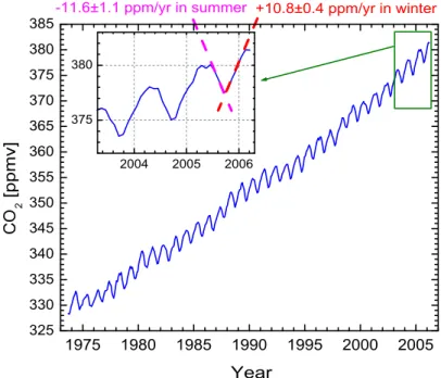
Mauna Loa (MLO) and Samoa (SMO) (Fig.1) was a suitable approximation of the mean CO2in air lofted into the upper troposphere (“CO2Index”, data updated by T. Conway).
ACPD
7, 6655–6685, 2007The CO2tracer clock for the TTL S. Park et al. Title Page Abstract Introduction Conclusions References Tables Figures ◭ ◮ ◭ ◮ Back Close
Full Screen / Esc
Printer-friendly Version
Interactive Discussion
EGU
“CO2clock” for tracing the time since air left the near-surface environment and entered the TTL. The seasonal slope in January and February (+10.8±0.4 ppmv yr−1, see inset
of Fig. 1 with expanded time axis) implies an increase of ∼28–30 ppb day−1. The Harvard CO2instrument has resolution of 50–100 ppb (Daube et al., 2002) enabling it
to distinguish mean age differences as short as 2–3 days.
5
This paper presents high-resolution, in situ observations of CO2 concentrations to
define the residence time and ascent rates for air in the TTL. We identify source regions for air entering the TTL and provide definitive time scales for TTL transport process by developing and validating the concept of the CO2tracer clock. The CO2measurements
in the TTL were carried out on a series of flights of the NASA WB-57F aircraft over
10
Costa Rica and adjacent ocean areas during the NASA Pre-Aura Validation Experiment (Pre-AVE) and Costa Rica AVE (CR-AVE) in January and February, 2004 and 2006, respectively. A large number of other tracer and meteorological measurements were made on the aircraft, providing important information on the chemical and dynamical context of the sampled air. The AVE missions give the first comprehensive tracer
15
data for the TTL. During the same flight period as CR-AVE, we also obtained in situ CO2 data on board the Proteus aircraft, from the Planetary Boundary Layer (PBL) up to 15 km over Darwin (12◦S), Australia (part of Tropical Warm Pool International Cloud Experiment, TWP-ICE). These data allow the first inter-hemispheric comparison of CO2composition of the TTL.
20
We present our extensive CO2 observations of the TTL in the context of the
char-acteristics of TTL structure and transport. First, instrumental information is given in the following section. In Sect. 3.1, the CO2 vertical profiles from CR-AVE are shown in potential temperature coordinates. In Sect. 3.2, we present the observed varia-tions/anomalies in the CO2 profiles in the lower TTL region below 360 K that can be 25
explained mainly by influence of local and/or remote convective inputs. In Sect. 3.3, we discuss the validity of the CO2tracer clock in the upper TTL region between 360 and
390 K and provide a direct measure of the mean vertical ascent rate and mean age of air transiting the TTL and entering the stratosphere.
ACPD
7, 6655–6685, 2007The CO2tracer clock for the TTL S. Park et al. Title Page Abstract Introduction Conclusions References Tables Figures ◭ ◮ ◭ ◮ Back Close
Full Screen / Esc
Printer-friendly Version
Interactive Discussion
EGU
2 Measurements
Measurements of CO2 mixing ratios on the NASA WB-57F aircraft and on the
Pro-teus aircraft were made using nondispersive infrared absorption CO2analyzers flown
in many previous experiments (see Daube et al., 2002, for details). The instruments are calibrated often in flight, and have demonstrated a long-term precision of 0.1 ppmv
5
(Boering et al., 1995). The standards are calibrated directly against CO2 world
stan-dards from the National Oceanic and Atmospheric Administration/Earth System Re-search Laboratory (NOAA/ESRL), and thus are directly comparable to surface data from the ESRL global network, with accuracy better than 0.1 ppmv. Our analysis uses data for potential temperature, ozone, and condensed water content (CWC) from other
10
sensors on the WB-57F, and CH4 mixing ratios from Pre-AVE whole air samples. Air temperature and pressure were measured by the Meteorological Measurement Sys-tem (MMS) on board the aircraft, with the reported precision and accuracy of ±0.1 K and ±0.3 K, respectively, for temperature, and ±0.1 hPa and ±0.3 hPa, for pressure (Scott et al., 1990). These parameters were used to derive potential temperate with
15
an uncertainty of ∼2 K. In situ ozone measurements were made by the NOAA Dual-Beam UV Absorption Ozone Photometer (Proffitt and McLaughlin, 1983). At a 1-s data collection rate, measurement precision is ±0.6 ppbv (STP) and average uncertainty is ∼±5%. The Cloud Spectrometer and Impactor (CSI-Droplet Measurement Technolo-gies) is based on the technology of the Counterflow Virtual Impactor (CVI) (Twohy et
20
al., 1997) and was used to measure total condensed water content in the range from 0.001 to 5 g m−3. Whole air samples were collected with the National Center for At-mospheric Research (NCAR) Whole Air Sampler (WAS) (Flocke et al., 1999). Mixing ratios of CH4 on the WAS samples were measured using a Hewlett Packard model
5890 gas chromatograph fitted with a flame ionization detector (GC-FID). Calibration
25
was made against a 0.913±0.01 and a 1.19±0.01 µmol/mol NIST-certified SRM 1658a reference gas. Measurement precision is ±10 ppbv and accuracy is ±20 ppbv.
ACPD
7, 6655–6685, 2007The CO2tracer clock for the TTL S. Park et al. Title Page Abstract Introduction Conclusions References Tables Figures ◭ ◮ ◭ ◮ Back Close
Full Screen / Esc
Printer-friendly Version
Interactive Discussion
EGU
3 Results and discussions
3.1 CO2observations from CR-AVE
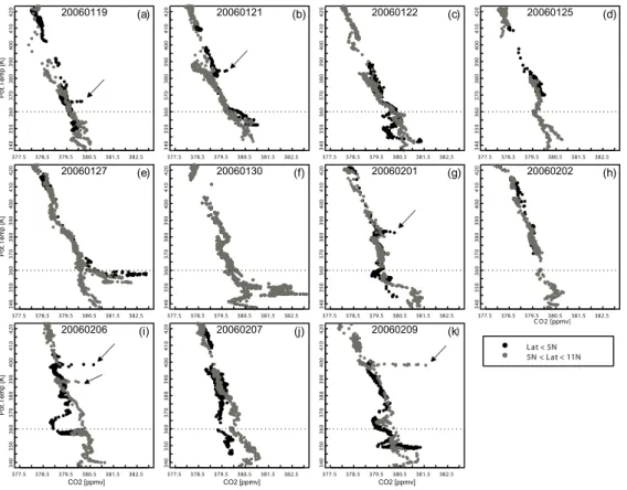
Measurements of CO2during CR-AVE are plotted in potential temperature (θ) coordi-nates in Fig. 2. Data from 11 science flights that sampled in the deep tropics, south of 11◦N are grouped by latitude, less than 5◦N in black and 5–11◦N in gray, flight-by-flight.
5
For all 11 profiles, the observed CO2 mixing ratios in general decline with increasing potential temperature (i.e., altitude) throughout the observed range of ∼330–430 K. Aircraft contrails (denoted by arrows in Fig. 2) and associated inputs of CO2from
com-bustion were readily detected.
Most of the CO2 vertical profiles for potential temperature < ∼360 K reveal consid-10
erable variations with either low CO2 bulges or high CO2spikes, or both (for example,
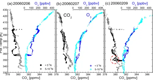
see the flights of 22, 27, and 30 January and 1, 6, 7, and 9 February). Variability is much less above 360–370 K. For the flights on 6, 7, and 9 February (Figs. 2(i), 2(j), and 2(k), respectively), low CO2bulges are most apparent, by ∼1.5 ppmv at ∼360 K, at the
southern end of the flights, i.e., only latitudes less than 5◦N. Figure 3 shows that these 15
bulges correspond perfectly with elevated O3, a stratospheric tracer, implying
substan-tial intrusion of lower stratospheric air at the southern end of the flights for those dates: this intrusion brought older, stratospheric levels of CO2. However, other low CO2 excur-sions from other flights do not pick up any corresponding feature in O3(e.g., a low CO2
excursion marked by a circle in Fig. 3c) and these are discussed further in Sects. 3.2.2
20
and 3.2.3 below.
In contrast to the lower TTL below ∼360 K, CO2 profiles for potential temperature
between ∼360–390 K form a compact, linear line with a negative slope in most flights. The monotonic decline in the mixing ratio is very significant, indicating that air is ag-ing with altitude since the seasonal cycle is on the risag-ing branch in boreal winter (see
25
Fig. 1). Differences in some of the CO2profiles between <5◦N and 5–11◦N, from the
minimum temperature level (i.e., ∼380 K) to ∼390–400 K may also be discernable (see Figs. 2a, b and c). Slightly lower CO2 values at 5–11◦N seem to reflect influence of
ACPD
7, 6655–6685, 2007The CO2tracer clock for the TTL S. Park et al. Title Page Abstract Introduction Conclusions References Tables Figures ◭ ◮ ◭ ◮ Back Close
Full Screen / Esc
Printer-friendly Version
Interactive Discussion
EGU
horizontal mixing between the tropical and midlatitude stratospheric “overworld” (de-fined as the region above ∼380 K), but profiles at <5◦N were not affected. Differences
between <5◦N and 5–11◦N disappear above ∼400 K, the level where air enters the “tropical pipe”. At these altitudes, a transport barrier in the 15–30◦N latitude range restricts mixing of midlatitude air into the tropics (Neu and Plumb, 1999; Plumb, 1996).
5
The CO2 profiles in potential temperature coordinate suggest that the TTL is
com-posed of two layers with the distinctive features. The lower TTL, up to the level of ∼360 K (14–15 km), exhibits profiles with considerable daily and latitudinal variations. In Sect. 3.2, we detail how these observed anomalies in the profiles can be explained by convective influence. The upper TTL ranging from ∼360 K to ∼390 K (17–18 km;
10
slightly above the tropical tropopause) is by contrast characterized by a linear decline and a compact correlation between altitude and CO2 mixing ratio, regardless of flight
date and latitudinal range. We discuss in Sect. 3.3 the implication of this observation for interpreting air ascending motion of the region.
3.2 Lower TTL below 360 K
15
We show here that the CO2 variations observed in the lower TTL are indicating the
influences of (1) local convection near Central America, (2) convective input from Amaz ˆonia, and (3) remote, deep convection over south central/western Pacific. We demonstrate that this explanation is entirely consistent with the analyses from con-densed water content data, back trajectories, and CH4measurements.
20
3.2.1 Local convection
For the flights on 27 and 30 January (see Figs. 2e and f), we measured high CO2 spikes of 2–3 ppmv between 12–13 km (i.e., ∼350–360 K). The CO2maxima are about
383 ppmv which corresponds to the mixing ratio of the near-surface in the northern tropics near Costa Rica. The CO2 monthly averages at Barbados (RPB, 13◦N 59◦W), 25
ACPD
7, 6655–6685, 2007The CO2tracer clock for the TTL S. Park et al. Title Page Abstract Introduction Conclusions References Tables Figures ◭ ◮ ◭ ◮ Back Close
Full Screen / Esc
Printer-friendly Version
Interactive Discussion
EGU
(BMW, 32◦N 64◦W) ESRL stations reach up to 381.8–384.5 ppmv in January, 2006.
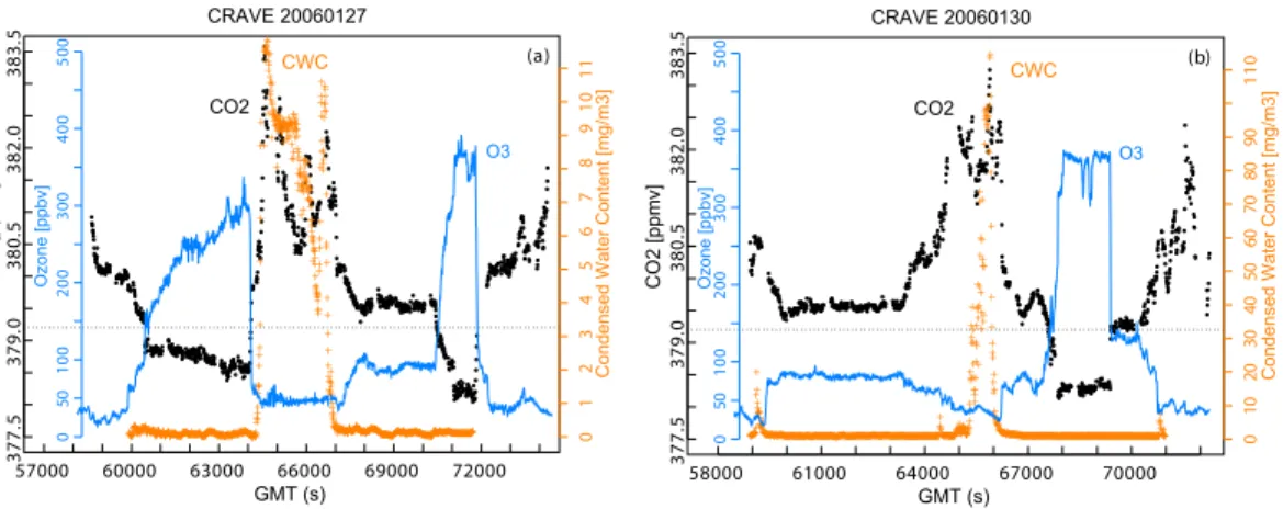
This implies a rapid injection of undiluted northern hemisphere tropical boundary layer air by deep convection to the level of 350–360 K. Figures 4a and b show typical CR-AVE flight segments on 27 and 30 January 2006. Note the correspondence with condensed water content in the outflow of a deep convective cloud, and the elevated CO2, which 5
is illustrating that we sampled wet air with high CO2 just outside a convective cloud.
Hence, cloud outflows constituting nearly undiluted air from the local boundary layer are clearly observed as elevated CO2in a number of instances, for potential temperatures
lower than ∼360 K.
3.2.2 Input from convection over Amaz ˆonia
10
The unexpected, but most interesting finding in the CO2 data from Pre-AVE in 2004 was the anomalously strong low CO2signals near 350 to 360 K of the vertical profiles
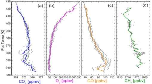
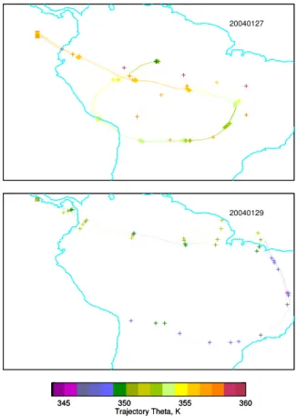
(Fig. 5a). These appear to be explained by the convective input from Amazon basin into the TTL (see Figs. 6a and b for back trajectories). Amaz ˆonian influence in the TTL was also observed in the CR-AVE CO2. As seen in Fig. 3c, a low CO2 excursion is 15
apparent near 350 K in the profile at <5◦N on 9 February, whereas O3 and CO gave
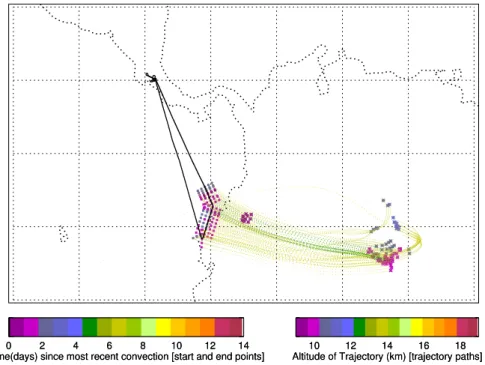
no corresponding hint of this feature. An independent analysis of back trajectory for CR-AVE (see Fig. 7) showed that this is a 2-day old air mass from Amaz ˆonia.
Other possible explanations for this low-CO2 feature can be rejected. If deep
con-vection reached up to the tropopause near 380 K, younger air in the upper TTL would
20
have more CO2 than older air in the lower TTL, as observed, but also CO should
increase with altitude, reflecting near-surface influence at the upper level. But CO concentrations decline with altitude, as shown in Fig. 5c. Another possibility might be stratospheric input, but we could not find any indication of elevated ozone (see Fig. 5b). In contrast to ozone and CO, the CH4 profile in Fig. 5d shows an anomaly, with 25
high CH4near 360 K corresponding to low CO2signals. The concentrations of CH4 in Amaz ˆonia are about 100 ppb higher than the global mean near the equator (J. Miller, personal communication, 2006), consistent with the observed enhancement. During
ACPD
7, 6655–6685, 2007The CO2tracer clock for the TTL S. Park et al. Title Page Abstract Introduction Conclusions References Tables Figures ◭ ◮ ◭ ◮ Back Close
Full Screen / Esc
Printer-friendly Version
Interactive Discussion
EGU
the transition from dry to wet season in late-January to early February, deep convection over Amaz ˆonia increases, occurring primarily in the afternoon (Liu and Zipser, 2005; Machado et al., 2004) when CO2 values are low (as low as ∼375 ppmv; L. Hutyra,
personal communication, 2006) due to the forest uptake. Thus deep convection over Amaz ˆonia brings CO2-depleted air to the TTL in contrast to inputs from local convection
5
discussed in Sect. 3.2.1 above. There is little biomass burning at this season, hence no enhancement is observed in CO.
We note that input to the TTL by deep convection over Amaz ˆonia was evident in CO2 observations in both Pre-AVE and CR-AVE, suggesting that this process may
be typical of the January-February time period. Amaz ˆonian influence in the TTL is
10
potentially very important for the chemistry of the TTL and lower stratosphere, in terms of excess reactive hydrocarbons and CH4 that the convective input must carry to the
TTL. This finding highlights the importance of multiple-tracer measurements including CO2, CH4and CO, since these tracer observations together can provide the capability to distinguish source air in the TTL from deep convection over tropical forests versus
15
the ocean and then to infer a quantitative measure of these influences. Quantitatively defining source regions that supply trace gases and H2O to the TTL would potentially allow us to address long-term changes in the humidity and aerosol content of the TTL and lower stratosphere.
3.2.3 Influence of remote convection over the Western/Central Pacific
20
Flights on 22 January and 1 February (see Figs. 2c and g) recorded low CO2 excur-sions observed near 350 and 355 K that cannot be explained by either local convection (CO2would be high) nor by Amaz ˆonian input, since CH4is low. The origins of low-CO2
air were examined using 10-day back trajectory analysis that tracked the air envelope surrounding ±0.5 km from the aircraft track to calculate statistics of air clusters
influ-25
enced by convection for the last 10 days (Pfister et al., 2001). A significant fraction of air cluster points from those low-CO2 air masses shows non-zero convective influ-ence in the central Pacific, i.e., the northern part of the South Pacific Converginflu-ence
ACPD
7, 6655–6685, 2007The CO2tracer clock for the TTL S. Park et al. Title Page Abstract Introduction Conclusions References Tables Figures ◭ ◮ ◭ ◮ Back Close
Full Screen / Esc
Printer-friendly Version
Interactive Discussion
EGU
Zone (SPCZ), off the northeast Australian coast, and in the New Guinea/Indonesia re-gion. Evidently we sampled remnant air from convection over the south central and/or western Pacific.
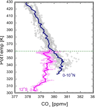
The CO2composition of air originating from the south central/western Pacific can be examined from our CO2 data obtained during TWP-ICE. Figure 8 shows the vertical 5
CO2 profiles from the flights on 25, 27, and 29 January 2006, over the south western
Pacific (12◦S, 130◦E). The Proteus aircraft sampled from near the surface (altitude of ∼1 km, ∼300 K) up to around 15-km altitude (i.e., ∼360 K). The CO2 mixing ratio at
∼1 km was between 378.1 and 378.8 ppmv, increased to the range between 379 and 380 ppmv below ∼4 km, and then stayed nearly constant with altitude to the aircraft’s
10
ceiling. Note strong contrast with the boundary layer CO2 composition in the north-ern tropics near Costa Rica (381.8–384.5 ppmv). Thus, convective input will cause excursion to either low or high CO2 in the profiles as observed for CR-AVE,
depend-ing on whether it originates from the southern tropical marine boundary layer or from nearby northern hemisphere tropical region, respectively. Hence, we infer that the low
15
CO2excursions of CR-AVE flights on 22 January and 1 February were due most likely
to remote, convective influence on the TTL of southern marine boundary layer air, in agreement with back trajectory results. It is also noted that the convective influences remained measurable for several days (i.e., ∼7–9 days; an estimate from the trajectory analysis) in the TTL, and were readily detected by CO2.
20
Clear concentration gradients between the southern and northern hemispheres are found from the surface to the upper troposphere and lower TTL. In Fig. 8, the TWP-ICE observations are shown along with the measurements from CR-AVE, allowing the first inter-hemispheric comparison in CO2mixing ratio between the southern and northern
parts of the TTL. Interestingly, the strong contrasts that are apparent in the upper
tro-25
posphere and lower TTL region disappear near 360 K: the CO2composition at ∼360 K in the southern tropics over Australia is very close to that in the northern tropics over Costa Rica. This result implies that the lower TTL below 360 K is subject to convective influence from boundary layer, but a global CO2signal emerges near 360 K in the TTL,
ACPD
7, 6655–6685, 2007The CO2tracer clock for the TTL S. Park et al. Title Page Abstract Introduction Conclusions References Tables Figures ◭ ◮ ◭ ◮ Back Close
Full Screen / Esc
Printer-friendly Version
Interactive Discussion
EGU
evidently the result of inter-hemispheric mixing in the Intertropical Convergence Zone (ITCZ). The average CO2 concentration of 380.0 (±0.2) ppmv at 360 K is somewhat
closer to the southern tropical boundary layer air, in accord with the ITCZ location in the southern hemisphere during NH winter. CO2measured at southern/central tropical, ESRL stations – Mahe Island (SEY, 4◦S 55◦E), Ascension Island (ASC, 7◦S 14◦W),
5
Samoa (SMO, 14◦S 170◦W), Cape Grim (CGO, 40◦S 144◦E), and Christmas Island (CHR, 1◦N 157◦W), averaged 379.9 (±1.3) ppmv in January, 2006, and an average of CO2 data for the northern tropical stations, Guam (GMI, 13◦N 144◦E) and Mauna
Loa (MLO, 19◦N 155◦W) was 381.4 (±0.3) ppmv. It suggests that we observed zero-age air occurring near 360 K during the CR-AVE time period, with dominant influence
10
from the ITCZ in the southern/central tropics. The TWP-ICE observations and their comparison with CR-AVE highlight the importance of obtaining complete vertical pro-files, including the boundary layer, in order to separate the diverse influences on the chemical composition of the TTL.
3.3 Upper TTL between 360 and 390 K
15
3.3.1 Level of 360 K
Based on the AVE and TWP-ICE CO2 data presented above, the level of ∼360 K is
suggested as the ceiling for significant input of air by convection from the boundary layer. Back trajectory analyses to convective systems, based on the method of Pfister et al. (2001), confirm this. These analyses compute the fraction of air cluster points
20
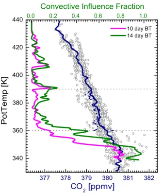
with non-zero convective influence for the back trajectory time (i.e., 10 and 14 days). Figure 9 shows that the convective influence fraction in 1-K average for all CR-AVE flights is concentrated mainly in the lower TTL, rapidly reducing to low values above 360 K. Back trajectories of 10 and 14 days both show the same pattern of a dramatic decrease in convective influence near 360 K. For the higher levels (near 390 K and
25
410 K), the occasional impact of convection seems to appear in the convective influ-ence fraction, but not in the CO2profile. This convective effect might explain observed
ACPD
7, 6655–6685, 2007The CO2tracer clock for the TTL S. Park et al. Title Page Abstract Introduction Conclusions References Tables Figures ◭ ◮ ◭ ◮ Back Close
Full Screen / Esc
Printer-friendly Version
Interactive Discussion
EGU
enrichment of water vapor isotopologues (e.g., Gettelman and Webster, 2005; Moyer et al., 1996; Smith et al., 2006) above and below the tropopause, which was in contrast to continuous isotopic depletion with altitude expected from Rayleigh fractionation model while air rises. A small input of ice from evaporation can have a big effect on water vapor isotopologues, whilst the influence on CO2is hard to discern unless a significant 5
fraction of the air is affected.
In addition, back trajectories of Fueglistaler et al. (2004) identified the maximum residence time of air parcels in the TTL as being at the level of ∼360 K. These authors explained that the level of zero clear sky radiative heating, where radiative balance changes from cooling to heating, occurs at ∼360 K (near 15 km), producing a so-called
10
stagnation surface in the vertical velocity. Above that level, radiation becomes more important than convection in regulating the mass flux of air. Disappearance of the inter-hemispheric difference in CO2 near 360 K, which is shown in Sect. 3.2.3 and
Fig. 8, can also be explained by effective horizontal mixing along the stagnation level with minimum vertical velocity.
15
3.3.2 CO2tracer clock
A nearly linear decline in CO2 mixing ratio, tightly correlated with altitude, was char-acteristic of the upper TTL (Fig. 2). Figures 8 and 9 showed that all CR-AVE CO2 data form nearly identical profiles with a negative vertical gradient. Large-scale, slow upward movement and monotonic aging of air while ascending are implied by these
20
CO2data, based on the rising phase of the CO2seasonal cycle in winter. The compact correlation of CO2 mixing ratio with altitude (i.e., potential temperature) indicates fast
horizontal mixing compared to vertical mixing. The youngest air, with near 0 age, is found at the base of the upper TTL (i.e., ∼360 K), representing a global mean CO2
composition (see Sect. 3.2.3), as opposed to air below that level showing strong
inter-25
hemispheric contrast in CO2 composition (Fig. 8). Moreover, air entering the upper
TTL retains imprint of the global seasonal cycle derived from the CO2 Index (Fig. 1), as inferred by Boering et al. (1996).
ACPD
7, 6655–6685, 2007The CO2tracer clock for the TTL S. Park et al. Title Page Abstract Introduction Conclusions References Tables Figures ◭ ◮ ◭ ◮ Back Close
Full Screen / Esc
Printer-friendly Version
Interactive Discussion
EGU
These results give rise to the idea of a CO2 “clock” for the TTL to infer a mean age and ascent rate of air using CO2data from the deep tropics (<11◦N). The CO2 tracer
clock estimates the mean age of an air parcel in the upper TTL from the time delay between the mixing ratio observed (or inferred) at the base (∼360 K) and the mixing ratio measured in the air parcels above 360 K, with the time scale identified by the
5
seasonal rates of change (i.e., slope of the seasonal cycle). Note that the inferred age is a true mean age representing the first moment of an age spectrum – the probability distribution function of times since air was last in contact with the surface (Hall and Prather, 1993; Waugh and Hall, 2002) – and it does not imply that all air parcels have the same history. The distribution of ages and transit times cannot be determined from
10
CO2data alone.
For January/February, the value of CO2 vertical gradient (∆CO2) and associated
age difference between 360 and 390 K were derived in the two following ways. First, in each flight, we selected CO2 values at 360 and 390 K and took their difference. The average and its 1σ uncertainty of the individual differences are stated as ∆CO2 15
between 360 and 390 K, 0.78(±0.09) ppmv. The value of ∆CO2 can also be obtained
from the slope of the plot of CO2 as a function of potential temperature in the range between 360 and 390 K, using a geometric mean regression which accounts for errors in both the x and y variables (Ricker, 1973). The slopes averaged 0.84(±0.29) ppmv of ∆CO2, not statistically different from the first method. The CO2clock combining these 20
CO2gradients with the winter slope (+10.8±0.4 ppmv/yr) of the seasonal cycle yields a
mean age of air at 390 K of 26(±3) and 28(±10) days, respectively. Hence, one expects that zero-age air at 360 K would reach/pass the 390 K level in average in less than one month. Indeed, we sampled air with CO2 value at 390 K on 9 February identical to
the 397.5 ppmv which we measured at 360 K on 14 January, exactly 26 days earlier,
25
confirming this conclusion.
The mean ages derived from the CO2clock are in good agreement with recent
anal-ysis of Folkins et al. (2006). Incorporating ozonesonde O3data and satellite CO
ACPD
7, 6655–6685, 2007The CO2tracer clock for the TTL S. Park et al. Title Page Abstract Introduction Conclusions References Tables Figures ◭ ◮ ◭ ◮ Back Close
Full Screen / Esc
Printer-friendly Version
Interactive Discussion
EGU
they reproduced the observed seasonal cycles of O3and CO at the tropical tropopause between 20◦S and 20◦N, and also calculated “an elapsed time since convective de-trainment” at the altitude of 17 km, which can be interpreted as the age of air. The estimate of age was 40 days at 17 km during NH winter, but it was reduced to 25 days when modeled with correction for air mass export to extra-tropics. A trajectory analysis
5
in the TTL incorporating radiative ascent, deep convection and zonal and meridional transport (Fueglistaler et al., 2004) also estimated one month for the average transit time from θ=340 K to 400 K, reasonably consistent with the CO2clock.
Our mean age values of 26(±3) and 28(±10) days imply mean vertical ascent rates of ∼1.5(±0.3) and ∼1.4(±0.5) mm s−1, respectively, at θ=390 K. The vertical ascent rates
10
are notably higher than those (0.1–0.5 mm s−1) derived from calculations of the
merid-ional circulation using heating rates (e.g., Dessler, 2002; Jensen and Pfister, 2004). The radiative heating rates are computed with radiative transfer models using satellite and/or climatological data for radiatively active compounds, and the calculations in the TTL have large uncertainties due to the small net heating rates (i.e., small difference
15
between two large numbers). Also, transient thin cirrus clouds, whose presence is dif-ficult to detect, may alter average heating rates significantly. As estimated in Jensen et al. (1996), the radiative energy due to IR absorption by thin cirrus could lift air with vertical ascent rate as high as ∼2 mm s−1.
The preservation of the CO2 seasonal trend in a compact, linear form throughout
20
the upper TTL suggests that horizontal mixing is fairly effective compared to vertical mixing and that vertical advection dominates both vertical diffusion and the mixing in of older air from the extra-topics (i.e., the lowermost stratosphere) in this critical layer at the entry point of the stratosphere. We did not observed attenuation of the seasonal amplitudes near above 390 K (Boering et al., 1996), confirming little effect of horizontal
25
input of older air from the extra-tropics into this deep tropics. A simple advection-diffusion model calculation showed that the vertical advection-diffusion of stratospheric air had negligible influence on observed CO2. Trace influence of stratospheric air in the TTL
ACPD
7, 6655–6685, 2007The CO2tracer clock for the TTL S. Park et al. Title Page Abstract Introduction Conclusions References Tables Figures ◭ ◮ ◭ ◮ Back Close
Full Screen / Esc
Printer-friendly Version
Interactive Discussion
EGU
In contrast to CO2, these species have very strong gradients in mixing ratio between troposphere and stratosphere, e.g., ∼40 ppbv at 340 K vs. ∼400 ppbv at 430 K for O3
(see Fig. 3) and zero vs. ∼0.3 ppbv for HCl. These gases thus display small influences of stratospheric air
How much influence of recent convective injection could there be beyond the
large-5
scale, slow ascent of the upper TTL? The vertical distribution of convective influence fraction for the back trajectories (Fig. 9) may help address this question. We examine the impact of convection on CO2profiles in the upper TTL by assuming the convective
influence fraction of 10 day trajectory as the actual air fraction containing the most re-cent convective injection. We also assume two extreme cases for CO2in the convective
10
air: 378.5 ppmv obtained from the surface in the TWP-ICE flights, and 383 ppmv from the northern tropical boundary layer. The associated change in the CO2mixing ratios
after accounting for the convective influence fraction in each case is not statistically significant, because the input fractions are too small. The slopes for the CO2clock with a putative correction for convective influence, and without correction, all agree within
15
their 1σ uncertainties, as illustrated in Fig. 9. Therefore, the small amounts of con-vection that might introduce in the region above 360 K would not be expected to have an observable effect on the CO2vertical distribution, and thus not on CO2clock in the
region. This insensitivity results from the fact that the CO2 clock represents the true
mean age.
20
The operation of the CO2 clock in the northern hemispheric summer can be tested
in a preliminary way by examining CO2 data collected during Stratospheric Tracers
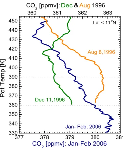
of Atmospheric Transport (STRAT) campaign in 1996. During STRAT, we sampled the lower tropical stratosphere and upper TTL over the central Pacific in December and August. The STRAT CO2 data shown in Fig. 10 are all consistent with the CO2 25
tracer clock, showing that the youngest air is at the base of the upper TTL and air is in slow rising above that level. Particularly, the vertical profile for August exhibited a CO2gradient reversed compared to December between 360 K and 380 K in STRAT or
ACPD
7, 6655–6685, 2007The CO2tracer clock for the TTL S. Park et al. Title Page Abstract Introduction Conclusions References Tables Figures ◭ ◮ ◭ ◮ Back Close
Full Screen / Esc
Printer-friendly Version
Interactive Discussion
EGU
seasonal cycle in NH summer (summer slope of –11.6 ppmv/yr; see Fig. 1). We expect the TC4 measurement program scheduled in July 2007 will help complete the tracer clock concept for NH summer and provide a seasonal constraint on the vertical trans-port rates for the TTL. Once the vertical ascent rate and the mean age inferred from CO2observations are well established, these parameters provide strong constraints to 5
help evaluate models and to help interpret satellite measurements that cannot resolve the vertical structure of the TTL.
4 Conclusions
The first extensive CO2data for the TTL, collected during Pre-AVE, CR-AVE, and
TWP-ICE, were used to determine the average source locations for air entering the TTL and
10
to define the time scales for air transport.
The in situ CO2 measurements show that the TTL is composed of two layers with
distinctive features: the lower TTL below 360 K, subject to inputs of convective outflows; and the upper TTL from ∼360 to ∼390 K, characterized by a compact, nearly linear decline in CO2mixing ratio with altitude. Observed variations in CO2vertical profiles for 15
the lower TTL are explained by the episodic influence of local and/or remote convective transport. Combining data for condensed water content, CH4, and back trajectories,
we could distinguish inputs of northern hemisphere boundary layer air from Central America and adjacent waters, Amaz ˆonian air, and the remote marine boundary layer air originating from the south central/western Pacific.
20
In the upper TTL, the data enabled us to validate the operation of a CO2 tracer
clock performing in an apparently uniform manner in both hemispheres. The first inter-hemispheric comparison in CO2composition of the TTL revealed that strong contrast between the hemispheres persists from the surface to lower TTL, but seems to disap-pear at the level of ∼360 K. Therefore, air entering the upper TTL has been efficiently
25
mixed between the hemispheres, to give a CO2mixing ratio very similar to the average of surface stations in the ITCZ. Observations in this study reflect limited impact of the
ACPD
7, 6655–6685, 2007The CO2tracer clock for the TTL S. Park et al. Title Page Abstract Introduction Conclusions References Tables Figures ◭ ◮ ◭ ◮ Back Close
Full Screen / Esc
Printer-friendly Version
Interactive Discussion
EGU
mixing and input of convective air at the altitudes above 360 K. The level of 360K may be considered as an average top of convective input from the boundary layer in the deep tropics for NH winter.
The CO2 concentration at the level of 360 K had near zero age. Concentrations of
CO2 declined with altitude up to 390 K, implying large-scale, slow ascent and
mono-5
tonic aging of air in the upper TTL. The mean age of air entering the stratosphere in NH winter was 26±3 days. Chemical compounds with lifetimes shorter than ∼26 days are expected to be injected mainly at the 360 K level, and are unlikely to be trans-ported into the stratosphere unless deposited above the tropopause by some other pathway, e.g., by the small amounts of convective air that are indicated in Fig. 9. The
10
inferred mean vertical ascent rate in NH winter was 1.5±0.3 mm s−1 in the upper TTL,
notably higher than velocities computed from radiative heating rates using satellite and climatological data. This result implies that satellite/radar observations may tend to un-derestimate high, thin cirrus clouds in the TTL, among other factors that heat the air in radiative transfer models. We infer that clouds in the upper TTL are more likely to lead
15
to radiative heating rather than cooling, since they appear to drive uplift of air. Better description of cloud fields in radiative transfer models is evidently required to reproduce the observed CO2“clock”, and these revised models will move air more quickly through
the TTL and into the stratosphere.
Acknowledgements. We thank L. Hutyra and J. Miller for helpful discussions and the NASA
20
WB-57F pilots and crews for the dedicated efforts. This work was supported by NASA grants NAG2-1617 and NNG05GN82G to Harvard University.
References
Andrews, A. E., Boering, K. A., Daube, B. C., Wofsy, S. C., Hintsa, E. J., Weinstock, E. M., and Bui, T. P.: Empirical age spectra for the lower tropical stratosphere from in situ observations
25
of CO2: Implications for stratospheric transport, J. Geophys. Res., 104(D21), 26 581–26 596, 1999.
ACPD
7, 6655–6685, 2007The CO2tracer clock for the TTL S. Park et al. Title Page Abstract Introduction Conclusions References Tables Figures ◭ ◮ ◭ ◮ Back Close
Full Screen / Esc
Printer-friendly Version
Interactive Discussion
EGU Andrews, A. E., Boering, K. A., Daube, B. C., Wofsy, S. C., Loewenstein, M., Jost, H., Podolske,
J. R., Webster, C. R., Herman, R. L., Scott, D. C., Flesch, G. J., Moyer, E. J., Elkins, J. W., Dutton, G. S., Hurst, D. F., Moore, F. L., Ray, E. A., Romashkin, P. A., and Strahan, S. E.: Mean ages of stratospheric air derived from in situ observations of CO2, CH4, and N2O, J. Geophys. Res., 106(D23), 32 295–32 314, 2001a.
5
Andrews, A. E., Boering, K. A., Wofsy, S. C., Daube, B. C., Jones, D. B., Alex, S., Loewenstein, M., Podolske, J. R., and Strahan, S. E.: Empirical age spectra for the midlatitude lower strato-sphere from in situ observations of CO2: Quantitative evidence for a subtropical “barrier” to horizontal transport, J. Geophys. Res., 106(D10), 10 257–10 274, 2001b.
Boering, K. A., Dessler, A. E., Loewenstein, M., McCormick, M. P., Podolske, J. R., Weinstock,
10
E. M., and Yue, G. K.: Measurements of stratospheric carbon dioxide and water vapor at northern midlatitudes: Implications for troposphere-to-stratosphere transport, Geophys. Res. Lett., 22(20), 2737–2740, 1995.
Boering, K. A., Wofsy, S. C., Daube, B. C., Schneider, H. R., Loewenstein, M., and Podolske, J. R.: Stratospheric mean ages and transport rates from observations of carbon dioxide and
15
nitrous oxide, Science, 274(5291), 1340–1343, 1996.
Brewer, A.: Evidence for a world circulation provided by the measurements of helium and water vapor distribution in the stratosphere, Q. J. R. Meteorol. Soc., 75, 351–363, 1949.
Conway, T. J., Tans, P. P., Waterman, L. S., and Thoning, K. W.: Evidence for interannual variability of the carbon cycle from the National Oceanic and Atmospheric Administration/
20
Climate Monitoring and Diagnostics Laboratory global air sampling network, J. Geophys. Res., 99(D11), 22 831–22 855, 1994.
Daube, B. C., Boering, K. A., Andrews, A. E., and Wofsy, S. C.: A high-precision fast-response airborne CO2 analyzer for in situ sampling from the surface to the middle stratosphere, J. Atmos. Oceanic Technol., 19(10), 1532–1543, 2002.
25
Dessler, A. E.: The effect of deep, tropical convection on the tropical tropopause layer, J. Geophys. Res., 107(D3), 4033, doi:10.1029/2001JD000511, 2002.
Fischer, H., Brunner, D., Harris, G. W., Hoor, P., Lelieveld, J., McKenna, D. S., Rudolph, J., Scheeren, H. A., Siegmund, P., Wernli, H., Williams, J., and Wong, S.: Synoptic tracer gradients in the upper troposphere over central Canada during the Stratosphere-Troposphere
30
Experiments by Aircraft Measurements 1998 summer campaign, J. Geophys. Res., 107(D8), 4064, doi:10.1029/2000JD000312, 2002.
ACPD
7, 6655–6685, 2007The CO2tracer clock for the TTL S. Park et al. Title Page Abstract Introduction Conclusions References Tables Figures ◭ ◮ ◭ ◮ Back Close
Full Screen / Esc
Printer-friendly Version
Interactive Discussion
EGU R. A., May, R. D., Moyer, E. J., Rosenlof, K. H., Scott, D. C., Blake, D. R., and Bui, T. P.: An
examination of chemistry and transport processes in the tropical lower stratosphere using observations of long-lived and short-lived compounds obtained during STRAT and POLARIS, J. Geophys. Res., 104(D21), 26 625–26 642, 1999.
Folkins, I., Loewenstein, M., Podolske, J., Oltmans, S. J., and Proffitt, M.: A barrier to vertical
5
mixing at 14 km in the tropics: Evidence from ozonesondes and aircraft measurements, J. Geophys. Res., 104(D18), 22 095–22 102, 1999.
Folkins, I., Braun, C., Thompson, A. M., and Witte, J.: Tropical ozone as an indicator of deep convection, J. Geophys. Res., 107(D13), 4184, doi:4110.1029/2001JD001178, 2002a. Folkins, I., Kelly, K. K., and Weinstock, E. M.: A simple explanation for the increase in
rel-10
ative humidity between 11 and 14 km in the tropics, J. Geophys. Res., 107(D23), 4736, doi:4710.1029/2002JD002185, 2002b.
Folkins, I., Bernath, P., Boone, C., Lesins, G., N. Livesey, A. M. Thompson, Walker, K., and Witte, J. C.: Seasonal cycles of O3, CO, and convective outflow at the tropical tropopause, Geophys. Res. Lett., 33, L16802, doi:16810.11029/12006GL026602, 2006.
15
Fueglistaler, S., Wernli, H., and Peter, T.: Tropical troposphere-to-stratosphere transport inferred from trajectory calculations, J. Geophys. Res., 109, D03108, doi:03110.01029/02003JD004069, 2004.
Gettelman, A. and Forster, P. M. d. F.: A climatology of the tropical tropopause layer,, J. Meteo-rol. Soc. Jpn., 80, 911–924, 2002.
20
Gettelman, A. and Webster, C. R.: Simulations of water isotope abundances in the upper troposphere and lower stratosphere and implications for stratosphere troposphere exchange, J. Geophys. Res, 110, D17301, doi:17310.11029/12004JD004812, 2005.
Hall, T. M. and Prather, M. J., Simulations of the trend and annual cycle in stratospheric CO2, J. Geophys. Res., 98(D6), 10 573–10 581, 1993.
25
Highwood, E. J. and Hoskins, B. J., The tropical tropopause, Q. J. R. Meteorol. Soc., 124(549), 1579–1604, 1998.
Hoor, P., Fischer, H., Lange, L., Lelieveld, J., and Brunner, D., Seasonal variations of a mix-ing layer in the lowermost stratosphere as identified by the CO-O 3 correlation from in situ measurements, J. Geophys. Res., 107(D5), 4044, doi:10.1029/2000JD000289, 2002.
30
Jensen, E. and Pfister, L., Transport and freeze‐drying in the tropical tropopause layer, J. Geophys. Res., 109, D02207, doi:02210.01029/02003JD004022, 2004.
for-ACPD
7, 6655–6685, 2007The CO2tracer clock for the TTL S. Park et al. Title Page Abstract Introduction Conclusions References Tables Figures ◭ ◮ ◭ ◮ Back Close
Full Screen / Esc
Printer-friendly Version
Interactive Discussion
EGU mation and persistence of subvisible cirrus clouds near the tropical tropopause, J. Geophys.
Res., 101(D16), 21 361–21 376, 1996.
Liu, C. and Zipser, E. J.: Global distribution of convection penetrating the tropical tropopause, J. Geophys. Res., 110, D23104, doi:23110.21029/22005JD006063, 2005.
Machado, L. A. T., Laurent, H., Dessay, N., and Miranda, I.: Seasonal and diurnal variability of
5
convection over the Amazonia: A comparison of different vegetation types and large scale forcing Theor. Appl. Climatol., 78(1–3), 61–77, 2004.
Marcy, T. P., Fahey, D. W., Gao, R. S., Popp, P. J., Richard, E. C., Thompson, T. L., Rosenlof, K. H., Ray, E. A., Salawitch, R. J., Atherton, C. S., Bergmann, D. J., Ridley, B. A., Weinheimer, A. J., Loewenstein, M., Weinstock, E. M., and Mahoney, M. J.: Quantifying Stratospheric
10
Ozone in the Upper Troposphere with in Situ Measurments of HCl, Science, 304, 261–265, 2004.
Moyer, E. J., Irion, F. W., Yung, Y. L., and Gunson, M. R.: ATMOS stratospheric deuterated water and implications for troposphere-stratosphere transport, Geophys. Res. Lett., 23(17), 2385–2388, 1996.
15
Neu, J. L. and Plumb, R. A.: Age of air in a “leaky pipe” model of stratospheric transport, J. Geophys. Res., 104(D16), 19 243–219 256, 1999.
Pfister, L., Selkirk, H. B., Jensen, E. J., Schoeberl, M. R., Toon, O. B., Browell, E. V., Grant, W. B., Gary, B., Mahoney, M. J., Bui, T. V., and Hintsa, E.: Aircraft observations of thin cirrus clouds near the tropical tropopause, J. Geophys. Res., 106(D9), 9765–9786, 2001.
20
Plumb, R. A.: A “tropical pipe” model of stratospheric transport, J. Geophys. Res., 101(D2), 3957–3972, 1996.
Proffitt, M. H. and McLaughlin, R. L.: Fast-response dual-beam UV-absorption ozone photome-ter suitable for use on stratospheric balloons, Rev. Sci. Instrum., 54(12), 1719–1728, 1983. Ricker, W. E.: Linear regression in Fishery Research, J. Fish. Res. Board Can., 30, 409–434,
25
1973.
Schoeberl, M. R., Duncan, B. N., Douglass, A. R., Waters, J., Livesey, N., Read, W., and Filipiak, M.: The carbon monoxide tape recorder, Geophys. Res. Lett., 33, L12811, doi:12810.11029/12006GL026178, 2006.
Scott, S. G., Bui , T. P., Chan, K. R., and Bowen, S. W.: The meteorological measurement
30
system on the NASA ER-2 aircraft, J. Atmos. Oceanic Technol., 7(4), 525–540, 1990. Sherwood, S. C. and Dessler, A. E.: A model for transport across the tropical tropopause, J.
ACPD
7, 6655–6685, 2007The CO2tracer clock for the TTL S. Park et al. Title Page Abstract Introduction Conclusions References Tables Figures ◭ ◮ ◭ ◮ Back Close
Full Screen / Esc
Printer-friendly Version
Interactive Discussion
EGU Smith, J. A., Ackerman, A. S., Jensen, E. J., and Toon, O. B.: Role of deep convection in
establishing the isotopic composition of water vapor in the tropical transition layer Geophys. Res. Lett., 33, L06812, doi:10.1029/2005GL024078, 2006.
Stohl, A., Bonasoni, P., Cristofanelli, P., Collins, W., Feichter, J., Frank, A., Forster, C., Gera-sopoulos, E., Ga¨ggeler, H., James, P., Kentarchos, T., Kromp-Kolb, H., Kru¨ger, B., Land,
5
C., Meloen, J., Papayannis, A., Priller, A., Seibert, P., Sprenger, M., Roelofs, G. J., Scheel, H. E., Schnabel, C., Siegmund, P., Tobler, L., T. Trickl, Wernli, H., Wirth, V., Zanis, P., and Zerefos, C.: Stratosphere-troposphere exchange: A review, and what we have learned from STACCATO, J. Geophys. Res., 108(D12), 8516, doi:8510.1029/2002JD002490, 2003. Twohy, C. H., Schanot, A. J., and Cooper, W. A.: Measurement of condensed water content
10
in liquid and ice clouds using an airborne counterflow virtual impactor, J. Atmos. Oceanic Technol., 14, 197–202, 1997.
Waugh, D. W. and Hall, T. M.: Age of stratospheric air: Theory, observations, and models, Rev. Geophys., 40(4), 1010, doi:1010.1029/2000RG000101, 2002.
ACPD
7, 6655–6685, 2007The CO2tracer clock for the TTL S. Park et al. Title Page Abstract Introduction Conclusions References Tables Figures ◭ ◮ ◭ ◮ Back Close
Full Screen / Esc
Printer-friendly Version Interactive Discussion EGU 1975 1980 1985 1990 1995 2000 2005 325 330 335 340 345 350 355 360 365 370 375 380 385
-11.6±1.1 ppm/yr in summer +10.8±0.4 ppm/yr in winter
CO 2 [ppmv] Year 2004 2005 2006 375 380
Fig. 1. The global CO2seasonal cycle from (CO2-MLO + CO2-SMO)/2 (Boering et al., 1996)
using ESRL data (Conway et al., 1994, updated by T. Conway). The inset shows as expanded time axis with the CR-AVE time period.
ACPD
7, 6655–6685, 2007The CO2tracer clock for the TTL S. Park et al. Title Page Abstract Introduction Conclusions References Tables Figures ◭ ◮ ◭ ◮ Back Close
Full Screen / Esc
Printer-friendly Version Interactive Discussion EGU 3 4 0 3 5 0 3 6 0 3 7 0 3 8 0 3 9 0 4 0 0 4 1 0 4 2 0 377.5 378.5 379.5 380.5 381.5 382.5 Po t. T e mp [ K] 20060119 (a) 3 4 0 3 5 0 3 6 0 3 7 0 3 8 0 3 9 0 4 0 0 4 1 0 4 2 0 20060121 377.5 378.5 379.5 380.5 381.5 382.5 (b) 3 4 0 3 5 0 3 6 0 3 7 0 3 8 0 3 9 0 4 0 0 4 1 0 4 2 0 20060122 377.5 378.5 379.5 380.5 381.5 382.5 (c) 3 4 0 3 5 0 3 6 0 3 7 0 3 8 0 3 9 0 4 0 0 4 1 0 4 2 0 20060125 377.5 378.5 379.5 380.5 381.5 382.5 (d) 3 4 0 3 5 0 3 6 0 3 7 0 3 8 0 3 9 0 4 0 0 4 1 0 4 2 0 Po t. T e mp [ K] 20060127 377.5 378.5 379.5 380.5 381.5 382.5 (e) 3 4 0 3 5 0 3 6 0 3 7 0 3 8 0 3 9 0 4 0 0 4 1 0 4 2 0 20060130 377.5 378.5 379.5 380.5 381.5 382.5 (f) 3 4 0 3 5 0 3 6 0 3 7 0 3 8 0 3 9 0 4 0 0 4 1 0 4 2 0 20060201 377.5 378.5 379.5 380.5 381.5 382.5 (g) 3 4 0 3 5 0 3 6 0 3 7 0 3 8 0 3 9 0 4 0 0 4 1 0 4 2 0 C O2 [ppmv] 20060202 377.5 378.5 379.5 380.5 381.5 382.5 (h) 3 4 0 3 5 0 3 6 0 3 7 0 3 8 0 3 9 0 4 0 0 4 1 0 4 2 0 CO2 [ppmv] Po t. T e mp [ K] 20060206 377.5 378.5 379.5 380.5 381.5 382.5 (i) 3 4 0 3 5 0 3 6 0 3 7 0 3 8 0 3 9 0 4 0 0 4 1 0 4 2 0 CO2 [ppmv] 20060207 377.5 378.5 379.5 380.5 381.5 382.5 (j) 3 4 0 3 5 0 3 6 0 3 7 0 3 8 0 3 9 0 4 0 0 4 1 0 4 2 0 CO2 [ppmv] 20060209 377.5 378.5 379.5 380.5 381.5 382.5 (k) Lat < 5N 5N < Lat < 11N
Fig. 2. Vertical profiles of CO2from 11 scientific flights in the tropics (<11◦N) during CR-AVE.
Data from the deep tropics less than 5◦N are given in black and 5–11◦N in gray. Note aircraft
contrails are readily detected (marked by arrows). Horizontal dotted lines denote the level of 360 K. (a)–(k) represent the flights on 19, 21, 22, 25, 27 and 30 January and 1, 2, 6, 7, and 9 February 2006.
ACPD
7, 6655–6685, 2007The CO2tracer clock for the TTL S. Park et al. Title Page Abstract Introduction Conclusions References Tables Figures ◭ ◮ ◭ ◮ Back Close
Full Screen / Esc
Printer-friendly Version Interactive Discussion EGU 378 380 382 384 386 330 340 350 360 370 380 390 400 410 420 430 (c) 20060209 (b) 20060207 (a) 20060206 CO 2 O3 < 5o N 5-10o N Pot Temp [K] CO 2 [ppmv] 0 100 200 300 400 O3 [ppbv] 378 380 382 384 386 CO 2 [ppmv] 0 100 200 300 400 < 5o N 5-10o N O3 [ppbv] 378 380 382 384 386 CO 2 [ppmv] 0 100 200 300 400 O3 [ppbv]
Fig. 3. Vertical profiles of CO2(denoted by solid dots) and O3(by blue diamonds) on 6(a), 7(b), and 9(c) February. Low CO2bulges from <5◦N are responding to high ozone signals,
suggest-ing stratospheric air input. Note dotted circle on 9 February marks the air mass influenced from deep convection over Amazon basin, discussed in Sect. 3.2.2.
ACPD
7, 6655–6685, 2007The CO2tracer clock for the TTL S. Park et al. Title Page Abstract Introduction Conclusions References Tables Figures ◭ ◮ ◭ ◮ Back Close
Full Screen / Esc
Printer-friendly Version Interactive Discussion EGU 570003 60000 63000 66000 69000 72000 7 7 .5 3 7 9 .0 3 8 0 .5 3 8 2 .0 3 8 3 .5 GMT (s) C O 2 [ p p mv] CO2 (a) + + + + ++++++++++++++++++++++++++++++++++++++++++++++++++++++++++++++++++++++++++++++++++++++++++++++++++++++++++++++++++++++++++++++++++++++++++++++++++++++++++++++++++++++++++++++++++++++++++++++++++++++++++++++++++++++++++++++++++++++++++++++++++++++++++++++++++++++++++++++++++++++++++++++++++++++++++++++++++++++++++++++++++++++++++++++++++++++++++++++++++++++++++++++++++++++++++++++++++++++++++++++++++++++++++++++++++++++++++++++++++ + + + + + + + + + + + + + + + + + + + + + + + + +++++ + + + + + + + + + ++ + + + + + +++++++++ + + + + + + ++++++++++++++++++++ + + + ++++++++++ + + + + + ++++ + + + +++++ + + + + + + + + + + + + + + + + + + + + + + + + + + ++ + + + + + +++++ + + + + + + + + + + + ++ + + + + + ++++++++++ + + + + + + + + + + + + ++ + + + + + + ++++ + + + + ++ + + + + + + + + + + + + + + + + + + + + + + + + + + + + + + + + + + + ++ + + + + + + +++++++++++++++++ + + + + + +++++++++++++++++++++++++++++++++++++++++++++++++++++++++++++++++++++++++++++++++++++++++++++++++++++++++++++++++++++++++++++++++++++++++++++++++++++++++++++++++++++++++++++++++++++++++++++++++++++++++++++++++++++++++++++++++++++++++++++++++++++++++++++++++++++++++++++++++++++++++++++++++++++++++++++++++++++++++++++++++++++++++++++++++++++++++++++++++++++++++++++++++++++++++++++++++++++++++++++++++++++++++++++++++++++++++++++++++++++++++++++++++++++++++++++ 0 1 2 3 4 5 6 7 8 9 1 0 1 1 C o n d e n se d W a te r C o n te n t [mg /m3 ] CWC 0 5 0 1 0 0 2 0 0 3 0 0 4 0 0 5 0 0 O zo n e [ p p b v] O3 CRAVE 20060127 58000 61000 64000 67000 70000 3 7 7 .5 3 7 9 .0 3 8 0 .5 3 8 2 .0 3 8 3 .5 GMT (s) C O 2 [ p p mv] CO2 (b) + + + +++++++++++++++ + + + + + ++++++ +++++++++ + + + + ++++++++++++++++++++++++++++++++++++++++++++++++++++++++++++++++++++++++++++++++++++++++++++++++++++++++++++++++++++++++++++++++++++++++++++++++++++++++++++++++++++++++++++++++++++++++++++++++++++++++++++++++++++++++++++++++++++++++++++++++++++++++++++++++++++++++++++++++++++++++++++++++++++++++++++++++++++++++++++++++++++++++++++++++++++++++++++++++++++++++++++++++++++++++++++++++++++++++++++++++++++++++++++++++++++++++++++++++++++++++++++++++++++++++++++++++++++++++++++++++++++++++++++++++++++++++++++++ + + + + + ++++++++++++++++++++++++++++++++++++++++++++++++++++++++++++++++++++++++++++++++ + + + ++ + + + + + + + + + + + ++ + + + + + + + + + + + + + + + + + + + + + + + + + + + + + + +++++ + ++ + + + + + + + + + + + ++ + + + + ++++++++++++++++++++++++++++++++++++++++++++++++++++++++++++++++++++++++++++++++++++++++++++++++++++++++++++++++++++++++++++++++++++++++++++++++++++++++++++++++++++++++++++++++++++++++++++++++++++++++++++++++++++++++++++++++++++++++++++++++++++++++++++++++++++++++++++++++++++++++++++++++++++++++++++++++++++++++++++++++++++++++++++++++++++++++++++++++++++++++++++++++++++++++++++++++++++++++++++++++++++++++++++++++++++++++++++++++++++++++++++++++++++++++++++++++++++++++++++++ + + + + + + +++++++++++ 0 1 0 2 0 3 0 4 0 5 0 6 0 7 0 8 0 9 0 1 1 0 C o n d e n se d W a te r C o n te n t [mg /m3 ] CWC 0 5 0 1 0 0 2 0 0 3 0 0 4 0 0 5 0 0 O zo n e [ p p b v] O3 CRAVE 20060130
Fig. 4. Flight segments for CO2, O3and condensed water content (CWC) (a) on 27 January and (b) on the 30th. The CO2 peaks that correspond to CO2 spikes in the vertical profiles (Figs. 2e and 2f), are clearly responding to enhanced condensed water content in the outflow of convective clouds. Note high O3and low CO2mixing ratios on the stratospheric side. Horizontal dotted line represents a CO2level at the tropopause. Black, solid dots give CO2, blue lines for O3, and orange, cross symbols for CWC.
ACPD
7, 6655–6685, 2007The CO2tracer clock for the TTL S. Park et al. Title Page Abstract Introduction Conclusions References Tables Figures ◭ ◮ ◭ ◮ Back Close
Full Screen / Esc
Printer-friendly Version Interactive Discussion EGU 374 375 376 377 330 340 350 360 370 380 390 400 410 420 430 (d) (c) (b) (a) Pot Temp [K] CO 2 [ppmv] 50 100 150 200 250 300 350 O3 [ppbv] 40 60 80 100 120 CO [ppbv] 1710 1740 1770 1800 CH4 [ppbv]
Fig. 5. Pre-AVE (a) CO2, (b) O3, (c) CO, and (d) CH4 observations. Empty circles represent averages in 1-K intervals of potential temperature for each flight on 24, 27, 29, and 30 January 2004. 1-K averages including all the flights are denoted by solid lines. Note that low CO2values found at ∼350 and 360 K reflect deep convective input over Amaz ˆonia, carrying reduced-CO2
ACPD
7, 6655–6685, 2007The CO2tracer clock for the TTL S. Park et al. Title Page Abstract Introduction Conclusions References Tables Figures ◭ ◮ ◭ ◮ Back Close
Full Screen / Esc
Printer-friendly Version Interactive Discussion EGU 20040127 20040129 345 350 355 360 Trajectory Theta, K 345 350 355 360 Trajectory Theta, K
Fig. 6. Back trajectories that trace (a) the low-CO2 air masses at ∼360 K of the flight on 27
ACPD
7, 6655–6685, 2007The CO2tracer clock for the TTL S. Park et al. Title Page Abstract Introduction Conclusions References Tables Figures ◭ ◮ ◭ ◮ Back Close
Full Screen / Esc
Printer-friendly Version
Interactive Discussion
EGU
10 12 14 16 18
Altitude of Trajectory (km) [trajectory paths]
10 12 14 16 18
Altitude of Trajectory (km) [trajectory paths]
0 2 4 6 8 10 12 14
Time(days) since most recent convection [start and end points]
0 2 4 6 8 10 12 14
Time(days) since most recent convection [start and end points]
Fig. 7. Back trajectories that trace the low-CO2air masses at ∼350 K of the flight on 9 February 2006 to Amazon basin.
ACPD
7, 6655–6685, 2007The CO2tracer clock for the TTL S. Park et al. Title Page Abstract Introduction Conclusions References Tables Figures ◭ ◮ ◭ ◮ Back Close
Full Screen / Esc
Printer-friendly Version Interactive Discussion EGU 377 378 379 380 381 382 383 300 310 320 330 340 350 360 370 380 390 400 410 420 430 12oS 0-10oN
PotTemp [K]
CO
2[ppmv]
Fig. 8. Vertical profiles of CO2obtained during CR-AVE and TWP-ICE. TWP-ICE observations were plotted from ∼1-km to 15-km altitude on 25, 27, and 29 January 2006. The measurements were performed over the Western Pacific ocean (12◦S, 130◦E). All the data were averaged into
1-K intervals for each flight. Empty cycle denotes CR-AVE CO2and empty diamonds for TWP-ICE CO2. The overall 1-K averages for each mission are also shown in solid lines.
ACPD
7, 6655–6685, 2007The CO2tracer clock for the TTL S. Park et al. Title Page Abstract Introduction Conclusions References Tables Figures ◭ ◮ ◭ ◮ Back Close
Full Screen / Esc
Printer-friendly Version Interactive Discussion EGU 377 378 379 380 381 382 340 360 380 400 420 440 PotTemp [K] CO 2 [ppmv] 0.0 0.2 0.4 0.6 0.8 1.0 10 day BT 14 day BT
Convective Influence Fraction
Fig. 9. Vertical profiles of CR-AVE CO2and fraction of air cluster points with non-zero convec-tive influence, which was calculated by back trajectory analyses to convecconvec-tive systems, based on the method of Pfister et al. (2001). The pink and green lines show the 1-K averaged fraction of air clusters influenced by convection for 10 day and 14 day trajectories, respectively. To test the degree of convective influence on CO2distribution, CR-AVE CO2profile between 360 and 390 K is corrected for convective influence fraction of 10 day back trajectory. Convective air flux is assumed of two versions of CO2mixing ratios: 378.5 and 383 ppmv that are lower and upper limits. The corrected profiles are represented by dotted line (see text in Sect. 3.3.2). Symbols for CO2are same as in Fig. 8.
ACPD
7, 6655–6685, 2007The CO2tracer clock for the TTL S. Park et al. Title Page Abstract Introduction Conclusions References Tables Figures ◭ ◮ ◭ ◮ Back Close
Full Screen / Esc
Printer-friendly Version Interactive Discussion EGU 377 378 379 380 381 330 340 350 360 370 380 390 400 410 420 430 440 450 Jan- Feb, 2006 Lat < 11oN Dec 11,1996 Aug 8,1996
Pot Temp [K]
CO
2[ppmv]: Jan-Feb 2006
360 361 362 363CO
2[ppmv]:
Dec
&
Aug
1996
Fig. 10. Two profiles of CO2 in the TTL from the central Pacific obtained during STRAT are shown along with CR-AVE CO2. Data from winter (December) are remarkably consistent with data from CR-AVE. Note the reversed CO2 gradient in August and thus operation of the CO2 clock.