Dicke enhanced energy transfer via off resonant coupling y Christopher Black.

Dicke Enhanced Energy Transfer via

Off Resonant Coupling by

Christopher Black

Submitted to the Department of Electrical Engineering and Computer Science in Partial Fulfillment of the Requirements for the Degrees of

Bachelor of Science in Electrical Science and Engineering

and Master of Engineering in Electrical Engineering and Computer Science at the Massachusetts Institute of Technology

November 19, 2000 MASS UbJ

-i

NSTITUTE

Copyright 2000 M.I.T. All rights reserved.

JULiI

2001

LIBRARIES BARKER

Author

OD mei~ Electrical Engineering and Computer Science November 19, 2000 Certified by _ Peter Hagelstein pervisor Accepted by -Arthur C. Smith

Dicke Enhanced Energy Transfer via Off Resonant Coupling

By

Christopher Black Submitted to the

Department of Electrical Engineering and Computer Science November 19, 2000

In Partial Fulfillment of the Requirements for the Degrees of Bachelor of Science in Electrical Science and Engineering

and Master of Engineering in Electrical Engineering and Computer Science

ABSTRACT

This thesis examines the dynamics of energy exchange in a model for second-order (indirect) coupling through off-resonant states. Specifically, the model hosts a second-order transfer of energy between two collections of two level systems via an off-resonant oscillator. No first-order transfer of energy is possible because the systems are optically isolated. The entire system is placed into a low-frequency simple-harmonic-oscillator (SHO) which indirectly couples the two collections of systems. Therefore, if the SHO is removed there is no energy exchange.

The frequencies of the oscillator and two-level systems are different (off-resonant); therefore, the rates of exchange are expected to be quite low. This novel approach achieves measurable coupling through coherent enhancement analogous to Dicke's (1954) superradiance. This thesis examines the period and rate of energy-transfer between the isolated systems, and attempts to extract patterns that analytically depend upon the number of atoms in each cavity, the coupling strength, the photon level, and the off-resonant ratio parameter. The characterization that follows uses dimensionless quantities and therefore is applicable to many different applications of the model.

Thesis Supervisor: Peter Hagelstein

TABLE OF CONTENTS List of figures ... 6 List of Tables... 8 A cknowledgm ents ... 9 G lossary... 10 Gapter 1 Introduction... 11 (YAper 2 M odel... 15 H am iltonian ... 15

Pseudospin Atom ic M odel... 17

Representation of System States...18

D icke Algebra... 20

1-A tom Coefficients ... 20

M uti-Atom Coefficients... 21

(Apter 3 D ynam ics ... 24

Evolution of States ... 25

Energy Initialization... 27

Single-State Initialization of Energy Eigenvalues...27

Gaussian Initialization of Energy Eigenvalues ... 28

Im plem entation of G aussian Filter... 29

Capter 4 N um erical Im plem entation... 32

Com plete Basis Set ... 32

Finite Basis Set ... 33

Photon Level Span in Basis... 37

Chpter 5 Results I ... 42

O ne Atom in Each Cavity ... 44

Shape of O ne-Atom Curve ... 44

Param eter Trends ... 46

Coupling strength, g ... 46

Off-Resonant Energy Ratio, q7 ... 51

Analytic Representation of Period and Maximum Slope ... 53

Three Atoms in Each Cavity... 56

Many Atoms in Each Cavity ... 58

Chapter 6 Generalized Coherent States ... 60

Initialization ... 61

Maximization of Energy Transfer Velocity... 61

Localization of Wave Packet ... 62

Im plem entation ... 64

D erivation of K ... 64

Implementation of Velocity Operator ... 65

Chapter 7 R esults II... 67

Functionality and Reliability of Generalized Coherent State Initialization .... 67

Increasing the Number of Atoms, A , with the Generalized Coherent State A pproach... 69

haipter 8 Scaling Versus Coupling Strength...72

Stationary Development of New Coupling Parameter ... 72

Dynamic Development of New Coupling Parameter... 74

Scaling of Rate with New Coupling Parameter ... 75

ChApter 9 C onclusion ... 78

R esearch Issues... 79

A ppendices... 80

A. Dynamics-Evolution of System via Matlab Code ... 81

B. Hamiltonian Generator-Generation of Hamiltonian with M atlab Code ... 87

C. Coherent Constraints-Coefficient and Table Generators in M atlab Code ... 94

D. PositionMap-Three Dimensional Representation of State Occupation through Matlab Code...100

E. One-Atom Energy Oscillation Periods v/s Parameters...102

References...108 Index...109

LIST OF FIGURES

Nwnlber Page

Figure 1: Schematic of a gedanken experiment ... 12

Figure 2: (a) Top-level Diagram of Model (b) Functional Diagram of Model... 16

Figure 3: Expected Energy Evolution With and Without Coupling... 25

Figure 4: Coupling Map of Possible States... 35

Figure 5: Basis Numbering Convention... 36

Figure 6: System I-Average Occupation per Photon Level ... 38

Figure 7: System II-Ripple on the Second Segment, Instead of a Smooth D rop O ff ... 40

Figure 8: System III-The Curve Never Reaches the Second Segment (D rops off)... 40

Figure 9: System IV-Significant Ripple, and no Apparent Roll Off ... 41

Figure 10: Typical One-Atom Energy Transfer Curve with Red Sinusoid Superposed ... 45

Figure 11: Period and Maximum Slope of Energy Transfer v/s g (n = 10, q = 0.001)... 47

Figure 12: Period and Maximum Slope of Energy Transfer v/s n (g = 0.01, q = 0.01) ... 49

Figure 13: Energy Transfer Curve for High n Rqgime. Still Sinusoidal... 50

Figure 14: Period and Maximum Slope of Energy Transfer v/s q (g = 0.01, n = 100)... 52

Figure 15: Actual Period and Maximum Slopes versus Estimated Values over Coupling Strength g (n = 10, iq= 0.001) ... 55

Figure 16: Actual Period and Maximum Slopes versus Estimated Values over Photon number n (g = 0.01, q7 0.o1)... 55

Figure 17: Actual Period and Maximum Slopes versus Estimated Values over Coupling Strength g (n =10, q = 0.oo1) ... 56

Figure 18: 3-Atom Energy Transfer Curve, Illustrating Non-Linearity from Sinusoid ... 57

Figure 19: Prediction of Transfer Curve for Increasing Number Of Atoms... 59

Figure 20: Ideal Localization for Initial State in I and

Q

Figure 21: 1-Atom Energy Transfer Curve with Generalized Coherent State Initialization ... 68

Figure 22: 3-Atom Energy Transfer Curve with Generalized Coherent State Initialization ... 69

Figure 23: 4-Atom Energy Transfer Curve with Generalized Coherent State Initialization ... 70

Figure 24: Diagram of Generic Large System with Coupling Pathways

Outlined for One State: m.,n. ... 73

LIST OF TABLES

Nwnh-r Page

Table 1: Dicke Coefficients for Differing Number of Atoms ... 23 Table 2: Possible Coupling Pathways... 34 Table 3: Period Variation over Photon Level... 41 Table 4: Period and Maximum Slope of Energy Transfer v/s g (n and q fix4.. 48 Table 5: Period and Maximum Slope of Energy Transfer v/s n (g and q fixd).. 49 Table 6: Period and Maximum Slope of Energy Transfer v/s q (g and n fix4I).. 52

ACKNOWLEDGMENTS

The author wishes to thank Peter Hagelstein for the many ideas, insight, jar of peanut butter, futon, and intravenous caffeine setup. The author also wishes to thank John Fini for time above and beyond what was necessary, the numerous clear explanations, organizational input, and patience as I completed my thesis. Most important of all, special thanks go to my lovely wife, Heather. She was patient with me while I spent all my time researching; she provided moral support, took care of the kids and the housework, proof-read, and of course made regular batches of cookies. This task would not have been possible without her overwhelming assistance! Last of all, I would like to thank my kids, Rebecca and Andrew, for sacrificing my extra time with them so that I could complete my thesis.

GLOSSARY

coherent: All atoms transition together in the same direction. A coherent excitation is when all atoms excite simultaneously.

coherent state: This expression is usually used in reference to a SHO. The wave packet follows classical motion similar to a pendulum and the shape of the wave packet remains constant. The generalized coherent state created in this thesis looks like a coherent state; however, it quickly loses its coherent properties (as would a coherent state in a quartic well).

gedanken experiment: gedanken is German for thought. A gedanken

experiment refers to thinking through an experiment on paper.

off-resonance: If the energies/frequencies of coupled systems differ, their interaction is off-resonant.

sloshing: Energy dynamics that obscure the transfer of energy from system A to system B.

spinor: A two-element column matrix used to represent the general state of a spin-1/2 particle, or similarly (in pseudospin representation) used to represent the excitation state of a two-level system.

Chapter 1

INT

RQDUJCTIO()N

Scientists usually devise theory to explain existing physical systems that have not been described, or that need better, more accurate explanations.' This often provides us with tools to use the systems more effectively or more fully. However, sometimes it is useful to develop theory for systems that do not exist, in hopes that by understanding them we may bring them into existence. By understanding the underlying physics, researchers have been able to propose many new systems theoretically and then from the understanding gained by the theory, build them.

The system that we propose in this paper, as far as we know, does not exist. Hagelstein (1998) originally made the proposal in the late 1990s. The system investigates the use of coherent enhancement to strengthen a nominally weak process of off-resonant energy transfer. The model includes two off-resonant transfers, the first from a collection of two-level systems into an oscillator, and the second from the oscillator into a second collection of two-level systems. The two-level systems can represent a discrete transition for many different quantum systems; we use an atomic model, however the results are ubiquitous. Similarly, the oscillator can represent any system that rings with a lower frequency (necessary for coherent enhancement), such as a microwave field.

Hagelstein postulates that this system behaves similarly to coupled pendulums. If one pendulum is oscillating and the other at rest, after some time, the coupling

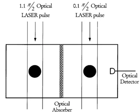
between the pendulums will transfer energy between them; therefore, the second pendulum will begin to oscillate. Eventually, the excitation from the first pendulum ideally is transferred to the second pendulum. The transfer of energy repeats itself and oscillates back and forth. Each pendulum may be ringing; however, independent of its motion, the overall energy oscillates between them. The pendulum illustration gives an easily understood and insightful representation of the system. We now proceed with a gedanken experiment (see Figure 1) to provide insight into the physical implementation of the model.

1.1 2 Optical LASER pulse 01 2 Optical LASER pulse Optical Absorber

Figure 1: Schematic of a gedanken experiment Figure from (Hagelstein 1999), used with permission.

Microwave

Cavity _Optical

This experiment uses atomic transition for the two-level systems and a microwave cavity for the oscillator. In a real system, the atoms would radiatively decay with a lifetime depending upon both the material and the discrete transition. We assume in our model that the coherent dynamics are much quicker than this lifetime. When implementing our system, this concern will affect the choice of materials for the gas.

Ignoring the decay mechanisms, our model predicts that excitation transfers between the two systems. However, this is not obvious from our setup, because the two cavities are optically isolated. The optical absorber is transparent to the microwave field, and so the exchange of energy occurs via the microwave field. The mechanism of exchange is resonant photons. One system emits an off-resonant photon, and the other system absorbs it. This channel of exchange is expected to be quite weak, so the expectation that these off-resonant processes should be significant goes against intuition, and demands more explanation. The weak indirect coupling between the collections of two-level systems may not be expected to satisfy our earlier assumption that the dynamics of exchange were quicker than the radiative-decay lifetime of the atoms. However, this is where our model differs from previous examinations of this type of effect. Since the wavelength of the oscillator is much longer than the optical cavity, we can generate substantial coherence factors. Therefore, the effective interaction strength is much larger than expected-directly analogous to Dicke superradiance (for more information see Dicke's paper (1954)).

The proposal of off-resonant supperradiant effects suggests a model for a system that does not yet exist. This theoretical exercise examines the plausibility of one such physical model. We believe that the theory demonstrates that the system is not only possible but also measurable, and that we may facilitate its existence with appropriate experiments. If the theory proves to be correct, this new physical

model would have many possible applications. We could create a laser that would exploit this ability to transfer by coupling a large system that is relatively unexcited into smaller systems. In addition, Hagelstein further suggest applications in spectroscopy, and up-conversion and down-conversion during nonlinear excitation transfer. (Hagelstein 1999)

Chapter 2

MODEL

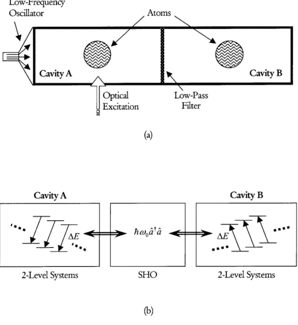
The model consists of three components: two cavities of gaseous atoms or molecules (two-level systems) that are isolated from each other, and an electromagnetic field (SHO) which is off-resonant. Figure 2 illustrates the system with two pictures: a structural diagram and functional diagram. The two cavities are identical; they each have the same number of atoms and equivalent coupling parameters. Initially, a laser excites Cavity A at the transition frequency. The atoms in the cavity are modeled as a collection of two-level systems; therefore, the excitation energy is chosen respective to the energy of the gas in the cavity. The electromagnetic field is any off-resonant field, such as a microwave, that can be modeled as an oscillator.

Hamiltonian

The total Hamiltonian models the collections of two-level systems, the oscillator, and the coupling between the components. The collections of two-level systems

(A and B) are isolated from each other; therefore, the coupling term between

them is zero. However, they each couple with the oscillator. Equation (2.1) shows an appropriate Hamiltonian for the system.

Two-Level Two-Level

Systems 'A' Systems 'B' Oscillator

A_-, Field

H = + ±A B +hca^ a

2 2 _(2.1)

+VA(a+ X a+VB a X

Coupling of 'A' Coupling of 'B' and Oscillator and Oscillator

Low-Frequency Atoms Optical 0UExcitation

S

2-Level Systems SHO

Cavity B

2-Level Systems

(b)

Figure 2: (a) Top-level Diagram of Model (b) Functional Diagram of Model

Oscillator

4(C avity A

h coo a

We use standard creation and annihilation operators to describe photon exchange in the oscillator. The resonant energy of the oscillator is hw,; its zero-state energy is unimportant, and consequently not modeled. The transition energy for the two-level systems is AE, and the model assumes that transitions in any atom are produced with equal probability. V, and VB represent the coupling strengths, and are equal for the described setup. The oscillator component of the coupling parameter is to the k power, which allows for higher order photon exchange. If a simple electromagnetic wave such as a microwave is used for the oscillator, k is equal to one; however, in other applications, for example atoms or molecules coupled to a phonon field, a higher order k of twenty or thirty may be necessary.

Pseudospin Atomic Model

The basic atomic model uses the same pseudospin formalism for the two-level systems as in Hagelstein's (1998) earlier paper. A two-element column vector (or spinor) models the two-level system. Each element represents one of the two states of the atom. If the value is one, then the atom is in that state; otherwise, it is equal to zero.

Unexcited:

1: _(2.2)

Excited:

0

The state vectors for the atoms multiply together to form a product state for the system.

(2.3) ya

For a single two-level atom, an arbitrary operator can be composed of the Pauli spin matrices -, and U,, &7. 3, leaves the atomic excited or unexcited state

invariant, and 8^ produces an atomic transition between the two states.

07L = (2.4)

10 11

&,

=L

A](2.5)

A + 0 1 0 0

Note: Ox =0++ ={ 0 + 0] (2.6)

To describe coherent excitation of many atoms, we use the following pseudospin operators:

ZZ W 0 -1 ,(2.7)

~I 0(=W 0[ I] (2.8)

Representation of System States

The two-element column matrix (or spinor) notation of equations (2.2) and (2.3) is not convenient when greater than a few atoms are used; therefore, we will use a simple notation to represent the system states. The eigenstates of the system depend not only on the number of atoms that are excited in each cavity, but also on the number of photons in the SHO; they in general look like

= I I CnM.Mb SaMa) I SbMb) (2.9) n Ma Mb

Three parameters are necessary to specify an eigenstate of the system: the photon level, n; the number of excited atoms in cavity A, M, ; and the number of excited atoms in cavity B, M2 . The photon number n is straightforward. The remaining

parameters, S and M , function

like

(Dicke,

AM = ±1 (2.10)

However, note that M is integral only if the number of atoms is even. From this formulation, physical definitions for S and M follow:

1 S = - Atoms (2.11) 2 1 M = -(AtomsEcited -AtomsUnexcited) (2.12) 2

(Note: The definition for S includes only the number of atoms in phase; if the atoms are out of phase, they cancel giving a lower effective S .)

Dicke Algebra

1-Atom Coefficients

The operators described above generate coefficients when applied to an eigenstate. Let us use an unexcited one-atom example to determine the coefficients created by these new operators. From equations (2.4) to (2.8), the one-atom operators are

2 =0,= 0] (2.13) 10 - I

S+=

[0

From equations (2.11) and (2.12) the initial eigenstate for an unexcited single-atom system is

#i =IS,M,)=

,

(2.16)

2 2

Let us first apply the normalized energy operator, (2.13), to the eigenstate, (2.16), to determine its coefficient.

2' = =l(-1)2(2.17)

(Note: in equation (2.17), the vector notation and the eigenstate notation is used interchangeably.) The coefficient from equation (2.17) is equal to 2M .

Z I S,M) = 2MIS,M) (2.18)

This relation holds for all values of S and M .

The x operator changes the state of the atom; therefore, since the atom is initially unexcited, applying the increment operator (2.14) yidds an excited atom.

S=0 ) = = _(2.19)

S2' 2 0 0 1 0 2'2

From equation (2.19), the coefficient for this single atom example is one. However, the coefficient changes depending upon the current state and the number of atoms; therefore, more examples are necessary to determine the analytic value of the coefficient.

Multi-Atom Coefficients

For the two-atom case

Q

(0

1

1

1 0 1 0 2222

Using equations (2.11) and (2.12), the initial eigenstate when both atoms are initially unexcited is

#

Applying operator (2.21) to the initial state (2.23) yieldsone excited atom and one unexcited atom.

0 0

]

_0 11_ +_0 1 2)-11-1012 =-111 .101 +1011 12

The final state has one excited and one unexcited atom, so 11,0) is the expected final state. Since, either atom can be excited with equal probability, 11,0) must combine and normalize both possible outcomes.

io=F1

1

1

F

1

1,]=2+ 0

[]1(2.25)

-v2 0 1 2 1- .02

Comparing equations

(2.24)

(2.25),

I'l 102 +l 10-12

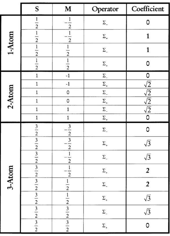
Table 1 includes all coefficients for up to three atoms. The general relation is:

Table 1: Dicke Coefficients for Differing Number of Atoms I U U

Operator

Coefficient

-

0

0

111

₀

o

-

I_

0

0

3-

₂

2

3

1

₂

2

2

S

M

Chapter 3

DYINA1tMICS

Chapter 2 gives us a framework for discussing energy in the three

subsystems-MI, M2, and n. This chapter examines the evolution of the energy in the

subsystems over time. The expectation of Z< and Z represents the instantaneous localized energies in the cavities. Therefore, by scaling, we can monitor the energy of the cavities through the excitation number, M . We define two new expectations.

2 z _(3.1)

In the absence of coupling, the system evolves trivially, (MI) and (M2) remain

constant. However, with coupling, we expect to see periodic transfer of energy between cavity A and cavity B. Figure 3 schematically illustrates the path we expect the energy to take. We are interested in the system with coupling, and specifically the details of the transition of energy from cavity A to cavity B. How sinusoidal is the transfer between the cavities? At what rate does it transfer? What system parameters define the period of motion?

Time Evolution of System -FT- - -- -T SMi witi - --- M2 wit -Mi wit M2 wit

-F

Figure 3: Expected Energy Evolution With and Without Coupling

Evolution of States

Outlining the periodic energy activity between the initial and final state requires examining the time evolution of the energy in the system. Beginning with a relevant basis of states

tta )

the resulting finite basis approximation for the H-amiltonian is found from

(3.3) 1 0.8 0.6 0.4 0.2 0 -0.2 0 0 A V cc -0. 4 A V -0.6 -0.8 -1 0 (3.2)

H.

The energies of the system are the corresponding eigenvalues of the finite basis matrix. Each eigenvector describes the energy contributions from each state. Therefore, solving the Hamiltonian (3.3) for eigenvalues and eigenvectors give

Vector

H v= Ek Vk (3.4)

Matrix S" ar

Let u be the probability amplitude of the system. u has a time-dependent component for each state of the basis, that component is the instantaneous probability amplitude of its respective state. For example, if the system is

initialized in the third basis state, (#3), then u (t = 0) is

0 0

1

u(t = 0)= 1(3.5)₀

0

We would like to make use of the following identity matrix:'

I = k)(k|= vkvk (3.6)

k k

SNote the symbol, I, in this context is not the 'dagger' operator but the adjoint operator. The adjoint of a vector/matrix is the complex conjugate transpose.

A)t = (A1

a1 At)=ad2+---+|a4|2 = 1

:=[a*---.a'*

nj NormalizedFor

Multiplying equation (3.5) by equation (3.6) gives:

u(0) = vkvk U(0) (3.7)

In vector form, equation (3.7) is a column multiplied by a row that is multiplied

by a column. The last two components, the row times a column, is a dot product

and simplify to a constant; therefore, it can be moved before the first column.

u(0)= [(vu())v] (3.8)

k

The evolution of this state vector is given by:

U(t)= e -u(0)= e h [(vlu(0))vk =ZI(vtu(0))e vI (3.9)

k k

Energy Initialization

The choice of u (0) in equation (3.9) significantly affects the dynamics of energy transfer. If the energy is initialized into states that do not couple with the set of states that we are interested in, then the evolution is trivial; because no energy ever evolves into the relevant states. Therefore, the initial state must be chosen carefully so that the energy is optimized to transfer back and forth from cavity A to cavity B.

Single-State Initialization of Energy Eigenvalues

One approach to initialization is to place all of the energy into a single basis state

excited, 1S,S)A S, -S)B , then we could expect that the energy would transfer to cavity B. Therefore, keeping the photon level at its center, this approach gives the following initial state:

S,S)A no)IS,-S)B

(3.10)

Let this be the 1th state of our basis,

#1

-n t

u, = v* l -e h vk , M

(.11

k vector I entry

Gaussian Initialization of Energy Eigenvalues

The initialization chosen in equation (3.11) is good because it guarantees that one of the states that we are interested in has energy; however, it is poor because it introduces extra sloshing to the system. Let us take a moment to clarify what we mean by 'extra sloshing'. When the system has many rapid dynamics that do not cause excitation from system A to system B, the transfer of energy appears somewhat chaotic. This chaotic energy transfer sloshes around; hence 'extra sloshing'.

We would like to eliminate the sloshing from the system. Initializing all the energy of the system into a single state is far from the system's equilibrium point; therefore, the system has extraneous rapid dynamics. If we initialize the system with the energy balanced similar to equilibrium; then we will significantly reduce

the extra sloshing. We attempt to simulate this effect with a Gaussian weighting of the eigen-energies for the system.

Implementation of Gaussian Filter

Let us begin by examining the effect of coupling using the eigenstates of the uncoupled system as a basis.

HO = -C# (3.12)

We can also write the coupled eigenstates.

(H + V)vj = Ejv, (3.13)

The proposal is to let

u'(t = 0)= E cjv (3.14)

where c. simulate the equilibrium conditions of the system. However, the system is rather complex, and we do not know the equilibrium spread of energy. Therefore, we can make an educated guess that it is close to a Gaussian, and let

cj = e-a(E-Ecenra)2 (3.15)

We expect a Gaussian to simulate the equilibrium point closely enough to see the periods clearly; however, a Gaussian is not sufficient by itself. We need an initial state that localizes energy in system A. Therefore, we combine the Gaussian weighting with the original basis state I#j).

2 iEkt

(

u(t)= N

kN

where the normalization constant N is

N.= ] 2 e-2a(E -Ecenter)2

and

B

Ecenter = i = Mean (E)

B

(3.16)

(3.17)

(3.18)

We want to favor cavity A so that the largest amplitude of oscillation is between cavity A and B. Therefore, we let the initial favored state be

,=

|S,S),n)|S,-S)B'

For a correct choice of the Gaussian parameter, a, this formulation successfully distributes the initial energy across the eigenvalues such that sloshing is minimal and the energy is mostly initialized in the proposed initial state, ii.

"In essence, choosing coefficients to resolve , = S, S), In) S, -SB leads to rapid dynamics that do not cause transfer of excitation from system A to system

B. We add a Gaussian filter to suppress this effect." (Hagelstein, personal

communication, October 27, 2000)

Chapter 4

NIUMERICAL

IMPT LEMEINTATI (YN

Complete Basis Set

Our next task is to choose a basis with which to work. The system has three degrees of freedom: M, M, and n. The size of the M-axes depends only upon the number of atoms in the system. M, and MB are identical in

construction. Each atom is either excited or unexcited (two states per atom); therefore, one would expect that the total number of states for each M-axis is

2A. However, all atoms in the system interact with the oscillator in the same

way, so they are indistinguishable from each other-either 0 atoms are excited, or

1, or 2,..., or A atoms. This is a total of A +1 states. We can also calculate

this value numerically from Dicke algebra. We know that M can change by the integer one, and ranges from -S to S:

M e

{-S,

A

Therefore, there are 2S +1 possible states for each M-axis. Since S = -,

2

# StatesM=#M =A+1 (4.2)

There are two dimensions for M , so the total cross-sectional state area for the M-plane is

#StatesM = #M -# (A 1)2 (4.3)

The size of the n-axis is infinite; there can be anywhere from zero to an infinite number of photons in the resonator.

Therefore, our complete basis set is a four-sided column of cross-sectional area

(A +1)2 that begins at n =0 and continues to infinity. Clearly, an infinite basis

set is not practical for this problem, nor computationally feasible. However, we can reduce the size of the basis once we examine the coupling pathways more closely.

Finite Basis Set

There are two states of particular interest in our problem. Initially, we are interested in all the atoms in cavity A being excited and cavity B unexcited. The other state of interest is the complement to the first state: all atoms in cavity A unexcited, and cavity B excited.

State I Cavity A: excited, IS, S), ; Cavity B: unexcited, S, -S)B

State II Cavity A: unexcited, S, -S), ; Cavity B: excited, IS, S)B

We are interested in these two states, because they are the endpoints of a complete energy transfer from cavity A to Cavity B. Let us begin with these two states as our finite basis, and then include those states that couple with them. Determining the states that couple, require us reexamine the Hamiltonian, equation (2.1). The first three components do not cause transitions (between basis states), and therefore can be ignored for this discussion; however, the last two terms do. The pseudo-spin operators change either the excitation parameter

in cavity A, MA , or in cavity B, MB, by one. Similarly, the creation and

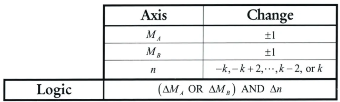
annihilation operators change the photon level, n; however, with the k-order parameter, the exchange is not as simple. The photon exchange can be any other number from -k to +k. For example, if k =1, then nne = n ±1; however, if

k = 2, then ne=0 or ±2. See Table 2.

Let us examine the one-atom case, A = 1, with k = 1. To facilitate the graphic

representation, we combine MA and MB into a single axis M . This is possible, since each axis is finite, and gives us a new axis of length (A + 1)2 = 4. Using a

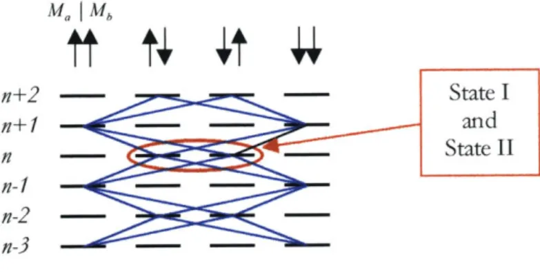
slightly modified M-notation of MA ,MB), State I and State II are now n) and , )n) Irespectively. From Table 2, we can say that State I

2 2 2 2

1 1 \

couples with four other states: - - - I)ln±1) and , In 1). Figure 4

2 2 2 2

maps out all states that couple with State I and State II for five photon levels. The coupling continues down to n =0 and up to n -> oo. The blue lines in Figure 4 represent the coupling pathways defined by the interaction Hamiltonian

(3.3). All other states may be excluded.

Table 2: Possible Coupling Pathways

Axis

Change

MA ±1

MB ±1

n -k,-k+2,,k -2, or k

M" | Mb n+2 4:State I n+1 - --- and n ___State II n-1 - - -n-2 - --n-3

-Figure 4: Coupling Map of Possible States

We have cut in half the number of states in the basis; however, it is still infinite. On the n-axis, the closer states couple stronger than the distant states, so if the contributions of these states become small enough, we can ignore them. However, what defines the coupling of a state to be small enough? This question depends upon the coupling strength, the photon level, and the off-resonant energy ratio. We determine it computationally by adding photon levels until the results do not change.

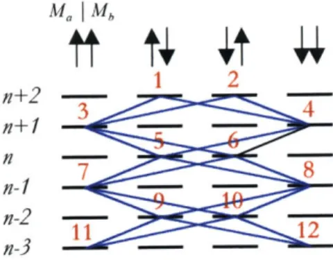
The convention this paper uses numbers the basis set from left to right and top to bottom, where only the states that couple (touched by a blue line) are included.

If the example that is in Figure 4 were used the basis would have 12 states; these

Ma I Mb

ttt4 t 4

Figure 5: Basis Numbering Convention

In Appendix B, matlab code is attached that creates a basis and calculates the respective Hamiltonian.

Photon Level Span in Basis

Each photon level added increases the total number of states by four. To simplify the following discussion, we define a new variable 1.

1 = n -no _(4.4)

Where no is the photon level of the system initially, and n is the photon level of the current state. We generate the basis symmetrically around the initial photon level, no; therefore, for a given 1, the span in n is 2/+1. To monitor the probability of occupation in each photon level, we sum the occupational probabilities of each state within a photon level and average over all time. Then we graph on a log-linear plot the sum versus relative photon level, 1. Such a graph tells us how many photon levels participate significantly, and how many must be included for accurate modeling.

There are typically two parts to every curve. The first segment does an initial drop and then wiggles around an occupation level up unto some 1. The second segment falls off exponentially. If we include enough states, at some 1 the curve eventually levels off due to truncation error within the computer; this is an artifact of the computer, not the quantum system. In the first segment, the occupation level is jumping around, and therefore, can still change the dynamics considerably (depending on the magnitude of the occupation). However, when the second segment of the curve begins its path becomes predictable, and we can anticipate any changes in dynamics. In other words, there will be no sudden period fluctuations when the basis is expanded past this point. The point, 1,

where the second segment of the curve begins (where its path becomes predictable) is the theoretical point we choose to accurately describe the dynamics of the system.

10

1, k = 1, Coupling Strength = 0.001, fl = 0.5, n = le+006

10--(U Significant Coupling C 1 0 0 CL 0 0 5 10 15 20 25 30 35 40 45 50

Photon Lemel Offset (I of n + 1)

Figure 6: System I-Average Occupation per Photon tnevel

See Figure 6 for a one-atom example of the photon curve. This curve uses single-state initialization with its initial parameters labeled above the graph. Notice the two segments of the curve that we have described. Based upon this graph, we would generally choose an 1 in the range of 20 to 30 for this system;

this choice is safely above the error threshold. The truncation error jumps

around, but its average value stays very constant. In addition, its occupation value will generally be below 10-2

Unfortunately, the photon curve is not always as clear as the above graph, so

choosing the breakpoint is not always possible or sufficient for accurate results.

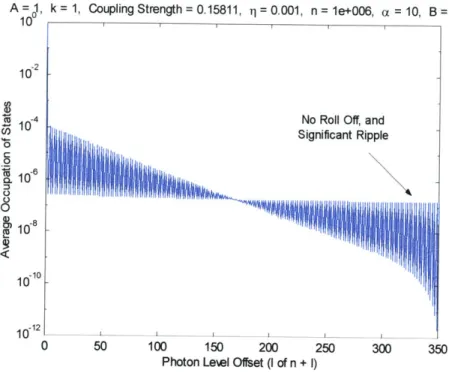
Figure 7, Figure 8, and Figure 9 show a few of these variations. The figures all have significant ripple on the smooth roll off section. Our argument is that we have included all significant coupling because the curve becomes predictable and smAg this is no longer true, for the occupation level bounces around what we

Smooth Roll Off, Negligible Coupling:

expect. Figure 8 adds another difficulty, for it does not reach the roll off section until / equals 260. This high value is computationally prohibitive for any atomic value other than one. Figure 9 also requires an enormous basis to reach the roll off point; furthermore, the jitter is large and does not attenuate.

First, we must quantify the error associated with the ripple. If the error is low enough, then it may allow us to reduce the number of photon levels that we generally include for a system. Let us first characterize how the period changes as we expand the number of photon levels included in the basis. Table 3 includes the four systems shown in Figure 6, Figure 7, Figure 8 and Figure 9 over important values of 1. Table 3 shows that it is quite possible to achieve good answers with even less photon levels than earlier proposed for many of the systems. However, System IV varies widely over the change in photon level; therefore, special care must be taken when the large characteristic zigzag of this system is seen. In the large coupling limit (when gva > 1), these zigzags

become more common, and significantly interfere with data collection. Unfortunately for the other systems, the measurement error of the periods is close to that shown between photon levels for each system. Therefore, we are less sensitive to the finite basis error and cannot achieve very precise mappings of the periods. However, our level of accuracy is more than sufficient to analytically define the system.

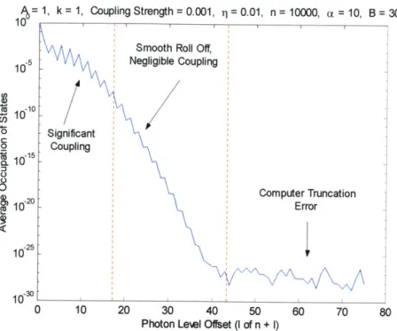
A= 1, k = 1, Coupling Strength = 0.001,

i h i= 0.01, n = 10000, a = 10, B = 302 Smooth Roll Off,

17 Negligible Coupling 10j ~10 o Significant Coupling 1015 0 _{Computer Truncation} 1C-20 Error 1072 1073 0 10 20 30 40 50 60 70 80

Photon Level Offset (I of n + 1)

Figure 7: System II-Ripple on the Second Segment, Instead of a Smooth Drop Off

1 = _{1, k =1, Coupling Strength =0.01, Tl=0.001, n =100, a 10, B = 1402} Roll Off, Negligible Coupling 10 0 CL Significant Coupling 5? 15 <10-10 0 50 100 150 200 250 300 350

Photon Level Offset (I of n + 1)

A = 1, k = 1, Coupling Strength = 0.15811, j = 0.001, n = le+006, a = 10, B = 1402

10

102

164 No Roll Off, and

Significant Ripple 0 C 0 0 10 107 1071 ---- ~ i_ 0 50 100 150 200 250 300 350

Photon Leel Offset (I of n + I)

Figure 9: System IV-Significant Ripple, and no Apparent Roll Off

Table 3: Period Variation over Photon Level

System Periods Versus 1

System I System II System III System IV

1 Period 1 Period 1 Period 1 Period

5 1.726 10 1.824-108 25 1.819 -107 20 8.6.107

20 1.724 25 1.823-108 50 1.824 .107 50 1.72 .107

35 1.724 40 1.821-108 100 1.817-107 100 4.3-106

50 1.724 75 1.816 .108 250 1.815 .107 200 1.6 -107

Chapter 5

RESULTS

I

The number of atoms, A ; the coupling strength, g ; the photon level of the oscillator, n ; and the ratio of energy between the systems (off-resonant ratio), q, affect the way the energy of the system evolves. Note that these parameters are normalized versions of our model:

h = _(5.1)

AE

g V (5.2)

AE

The normalized Hamiltonian is then

H A ~B _t

_ = t A+ )(

Hn AE 2 2 7'a'b(^ Ja X X (5.3)

We anticipate clear trends in the dynamics of the system that are analytic functions of these four parameters- A, g, n, and /7. For example, the stronger the coupling, g , the shorter we would expect the period of energy transfer between cavities to be, because the coupling pathway between cavities is more easily crossed. Similarly, as the number of atoms in a cavity increase, the Dicke coherence factors increase. The stronger the coherence factors the stronger the interaction between cavities, i.e. the effective coupling. Therefore,

we expect the periods to get smaller as A grows. Furthermore, when all atoms do interact coherently, we expect the rate of energy transfer to increase, because more atoms are transferring energy. Conversely, we expect that the more off-resonant the system and/or the higher the photon level, the larger the transfer period. These parameters are fundamental to the way the system operates; therefore, our results depend heavily upon the value of these parameters.

An analytic function that describes the period of transfer for this system is potentially very complicated. We would like to form a relation where each parameter's effect on the period is independent of all other parameters; or in mathematical terms, a separable function.

T(A,g,n,q) = fA (A)-fg (g)-fn (n)-f,(q) (5.4)

More realistically, the relation would include cross terms. For example,

fAg (Ag ) 1fA(A-n), (A 7), fgf(g n), fgq(g 7) (5.5)

and

fA( -g -n)

(A

Also, it might include any higher order variants

fA₂gn (A2g -n),f , (A .g2. n),--- (5.7)

To specify the answer exactly would be very complex, if possible. Therefore, this analysis empirically fits the curve with a low order approximation. The sources of error associated with this simplification are addressed subsequently.

One Atom in Each Cavity

Let us begin by setting up the system with one atom in each cavity. This eliminates any direct interaction between atoms, such as spin state cancellation (singlet and triplet states). In addition, all changes of state are completely coherent (all atoms in a cavity transition between their two excitation levels simultaneously).' With the number of Atoms, A, equal to one, the Dicke number, S , by equation (2.11) is

S =(5.8)

2 2

Shape of One-Atom Curve

An elementary problem analyzed in Quantum Mechanics is two coupled two-level systems. We know that the energy probability of this system oscillates between the two-level systems sinusoidally. In our model, one atom in each cavity is essentially two two-level systems coupled together with a slightly more involved coupling pathway. Therefore, we expect the shape of the one-atom curve to be similar to the Rabi oscillations of the simple case: sinusoidal. Figure

10 shows a typical one-atom curve with a red sinusoid superposed at the same

frequency and amplitude. Notice the similarity between the blue and red curves. As we suspected, the typical one-atom case is sinusoidal.

A model with two identical two-level systems has only four possible states;

therefore, it has four energy eigenvalues. Since both systems are identical with identical coupling each way, there are only two possible system frequencies:

jE - E2|=jE2- E3=co. and |E 1-E3j=2co. Our system, on the other hand,

1 However, note that the de-excitation is far from enhanced, because there is no coherent advantage given by only one atom.

A: 0 C (a x5 a 0.5 0.4 0.3 0.2 0.1 0 -0.1 -0.2 -0.3 -0.4 -0.5 1, k = 1, Coupling Strength = 0.01, = 0.001, n = 100, a = 10, B = 402 M1 M2 Sinusoid -I - --/ -/ 0 0.5 1 1.5 Time [s] 2 2.5 3 7, x 10 * hbr AE

Figure 10: Typical One-Atom Energy Transfer Curve with Red Sinusoid Superposed

couples via an oscillator; this adds an infinite number of states. Therefore, our system may have ripple and unclear periods when two system frequencies with significant amplitude are close in value. The high frequency ripple specifically make slope measurements difficult and inaccurate. However, since the shape is fundamentally sinusoidal, we may extract the slope of the line by integrating.

M(t)= Csin -- t (5.9)

M (t)=22r--os --- t (5.10)

Therefore, the maximum slope is 2)r times the amplitude over the period:'

C

Max slope = 2)r (5.11)

T

Parameter Trends

The coupling strength, photon level, and off-resonance affect the dynamics of the system. We have mapped out the periods and slopes over reasonable ranges for these parameters; the exhaustive results are in Appendix E. However, each parameter section includes a table extracted from Appendix E highlighting its respective trends.

Coupling strength, g

At the start of this chapter, we argued on physical grounds that the period would decrease as the coupling increased. Assuming this argument is true, we can argue that the maximum slope will increase by equation (5.11). Table 4 and Figuie 11 show that the data agree with our reasoning; the period changes inversely with g and the maximum slope, proportionally.

On the log-log plot of Figure 11, the period has a slope of negative two, therefore, the system is inversely proportional to g2_.

- g <0.1 Period

{

1 This formula does not hold for energy transfers that do not look sinusoidal, for example when two frequencies that are close together both have significant amplitudes.

The maximum slope, on the other hand, increases with a slope of one giving a proportional dependence of g.

Max Slope g2 g < 0.1

M g g>O.1 (5.13)

As we would expect from equation (5.11) the period and maximum slope mirror each other; therefore, the dynamics for the one-atom case remain sinusoidal for changing g.

Coupling Strength versus Period with n = 10 and 7 = 0.001

10 d

i

Figure 11: Period and Mlaximumn _{Slope of Energy Transfer v/s g} (n =10, r7= 0.001)

Table 4: Period and Maximum Slope of Energy Transfer v/s g (n and q7 fixed)

n g )q MaxSlope--

T----AE h

10 3.1623E-05 0.001 1.9970E-12 1.5730E+12

10 6.3246E-05 0.001 7.9538E-12 3.9300E+11

10 9.4868E-05 0.001 1.7860E-11 1.7400E+11

10 1.2649E-04 0.001 3.1806E-11 9.8400E+10

10 1.5811E-04 0.001 4.9927E-11 6.3000E+10

10 1.8974E-04 0.001 7.1611E-11 4.3700E+10

10 2.2136E-04 0.001 9.7906E-11 3.1000E+10

10 2.5298E-04 0.001 1.2722E-10 2.4600E+10

10 2.8460E-04 0.001 1.6117E-10 1.9400E+10

10 3.1623E-04 0.001 1.9945E-10 1.5700E+10

10 9.4868E-04 0.001 1.79E-09 1.7500E+09

10 1.5811E-03 0.001 4.9908E-09 6.2950E+08

10 2.5298E-03 0.001 1.2647E-08 2.4650E+08

10 3.1623E-03 0.001 1.9931E-08 1.5700E+08

10 3.1623E-02 0.001 1.6449E-06 1.8250E+06

10 1.5811E-01 0.001 6.8693E-06 2.3700E+05

10 2.2136E-01 0.001 7.5000E-06 1.7600E+05

10 3.1623E-01 0.001 7.6952E-06 1.2000E+05

10 6.3246E-01 0.001 8.5000E-06 5.7000E+04

Photon Level, n

We have suggested that the period will increase as the photon level increases, and therefore, the maximum slope will decrease. Table 5 and Figure 12 show that the period is proportional to n, and the slope inversely proportional. Specifically, at high n, the period grows as its square root; at low n, the period is unaffected.

T oc {

IE1

n>100

Normalized Period, T, and slope, m, of Energy Transfer Vs Photon Lemel, n

-0 - - 1- 3

10 10 102 103

Photon Lewl, n

10 10

Figure 12: Period and Maximum Slope of Energy Transfer v/s n (g 0.01, q = 0.01)

Table 5: Period and Maximum Slope of Energy Transfer v/s n (g and q fixed)

-I-M n g 77 MaxSlope- h T- AE AE h 1 0.01 0.01 1.9915E-06 1.5800E+06 10 0.01 0.01 1.9549E-06 1.6000E+06 100 0.01 0.01 1.6597E-06 1.8200E+06 1000 0.01 0.01 6.5264E-07 3.6700E+06 10000 0.01 0.01 7.7500E-08 1.2400E+07 30000 0.01 0.01 2.1500E-08 2.1000E+07 50000 0.01 0.01 1.2000E-08 2.8000E+07 80000 0.01 0.01 1.3362E-08 3.5710E+07 100000 0.01 0.01 7.8570E-09 3.9000E+07 200000 0.01 0.01 3.2660E-09 5.5000E+07 300000 0.01 0.01 1.4290E-09 6.7000E+07 500000 0.01 0.01 8.3333E-10 9.3000E+07 600000 0.01 0.01 5.0000E-10 1.0700E+08 800000 0.01 0.01 4.1667E-10 1.4500E+08 900000 0.01 0.01 3.3333E-10 1.8000E+08 1000000 0.01 0.01 1.6667E-10 2.OOOOE+08 10 10 10 10 8 z 10, -~~~ ---~ ~ -- - - ---- ---- - -- - - _{Period, T} --- -M----p---: --ZZ ----- -- -- ------ - - - - - - - - - - - - - ---- -- --- - -- ---- -- -- -- - - --- - - :- --- -- --- -- - ---- --- ---_{- - - - -- - - -} -10 107< E -7 107 _ F/, E E -8 -9 10 z 10

5

The maximum slope has a similar trend, it is constant at low n, and inversely proportional at large n. n >100 mn, oc In I n <100 (5.15)

This trend differs from what we expect. The maximum slope and period do not inversely track each other; therefore, it suggests that the transfer curve is not strictly sinusoidal. Figure 13 shows a curve in the high n regime and the transfer is still clearly sinusoidal; however, the amplitude is very low. The low amplitude of the transfer curve causes the discrepancy in the maximum slope. Equation

=1, k = _{1, Coupling Strength =0.01, rj=0.01, n =} 30000, a=10, B 402

-

M-Sinusoid M2

-/

0 0.5 1 1.5 2 2.5 3

Time (s) x 107

Figure 13: Energy Transfer Curve for High n Regime. Still Sinusoidal

A 0.11 0.1 .00 C 2 0 CU I -0.0 Or -0.1 -0.15 -0.2 - -- - " ..- - - - -- '= --

7.-(5.11) shows a direct dependence of the maximum slope on the amplitude of the

sinusoid. The amplitudes of most curves have been very similar with a value around 0.5; therefore, their periods and maximum slopes track inversely proportionally. The curve in Figure 13 is less than one fifth of the norm (-0.08). In the high n regime, the amplitude is no longer constant but decreases with n; therefore, this extra variable gives a discrepancy in the symmetry between the maximum slope and period.

Off-Resonant Energy Ratio, q

Fixing g and n and varying q shows a simple dependence on the off-resonance.

T oc (5.16)

MX Oc r7 (5.17)

The maximum slope and period trends in q clearly have a sinusoidal relationship. See Figure 14 and Table 6 below.

Period, T, and Maximum Slope, m , 's Off-Resonant Ratio Parameter, il 10 14 10 12 10 10s 10 8 10 10 - Period, T Max Slope, m -4 - -- --- --- L --- - -- --- .. .. .. ---... ----. .. 10 m=-1 m=+1 06 -- - --- - - --- --- _{--- - --- - - - ---} 1 -8 --- - - ---- ---- --- --- - - --- -- -- --- --- --- 1610 --- - --- -_- -_A10716 -10 10~ 10~ 10 100

Off-Resonant Ratio Parameter, i

Figure 14: Period and Maximum Slope of Energy Transfer v/s 7 (g = 0.01, n = 100)

Table 6: Period and Maximum Slope of Energy Transfer v/s q (g and n fixed)

h AE

ng 7 MaxSlope---

T---AE h

100 0.01 1.OOE-08 1.6596E-12 1.8200E+12

100 0.01 0.000001 1.6596E-10 1.8200E+10 100 0.01 0.0001 1.6596E-08 1.8200E+08 100 0.01 0.001 1.6596E-07 1.8200E+07 100 0.01 0.01 1.6597E-06 1.8200E+06 100 0.01 0.05 8.3108E-06 3.6300E+05 100 0.01 0.08 1.3329E-05 2.2600E+05 100 0.01 0.1 1.6697E-05 1.8100E+05 100 0.01 0.2 3.4161E-05 8.8000E+04 100 0.01 0.3 5.3709E-05 5.5400E+04 100 0.01 0.4 6.8190E-05 4.2900E+04 100 0.01 0.5 9.4014E-05 3.1100E+04 100 0.01 0.6 1.1142E-04 2.4000E+04 100 0.01 0.7 1.2395E-04 1.9700E+04 100 0.01 0.8 1.1667E-04 1.7200E+04 w E E E z w 0-*0 z F 10n-2

Analytic Representation of Period and Maximum Slope

Combining the parameter's lower-value regimes from the above results gives a very simple relation for the normalized period and slope.

T =18.2 (5.18)

917

Mg = 2z 2 f (5.19)

T

The maximum slope takes advantage of the sinusoidal shape of the transfer as described earlier. 6 is the average peak amplitude of the system. Ideally,

= 0.5 if all of the energy transfers between the systems; however, we use a

more realistic choice of 8 = 0.47. Note, as we have seen earlier, the use of a constant for

,8

We can improve our estimate by including the breakpoints in the above data for

g and n . The new expressions are

n 2 +14 g 2 2

z 200 0.04

T= -2- 7](5.20)