Dielectric Resonator Antennas : theory and design

Dielectric Resonator Antennas: Theory and Design

by

Beng-Teck Lim

Submitted to the Department of Electrical Engineering

in partial fulfillment of the requirements for the degree of

Master of Engineering in Electrical Engineering and Computer Science

at the

MASSACHUSETTS INSTITUTE OF TECHNOLOGY

February 1999

(Beng-Teck Lim, 1999. All rights reserved.

The author hereby grants to M.I.T. permission to reproduce and distribute publicly

paper and electronic copies of he thesis and to grant others the right to do so.

A A

Author

...

k

Department of Electrical Engineering

January 15, 1999 . I

Certified

Certified by

Ali Tassoudji

Qualcomm Inc.

J

Thesis Supervisor

Jin Au Kong

Professor

Thesis Supervisor

Accepted

by...;

;-

-

L._:."I...

. .-.

...

.

...

_{Arthur C. Smith}

Chairman, Department Committee on Graduate Theses

ARCHIVES

Dielectric Resonator Antennas: Theory and Design

by

Beng-Teck Lim

Submitted to the Department of Electrical Engineering

on January 15, 1999, in partial fulfillment of the requirements for the degree of

Master of Engineering in Electrical Engineering and Computer Science

Abstract

Theoretical models for the analysis of Dielectric Resonator Antenna (DRA) are developed. There are no exact solutions to many of the problems in analytical form, therefore a strong focus on the physical interpretation of the numerical results is presented alongside theoreti-cal models. I have used the physitheoreti-cal interpretation of the numeritheoreti-cal results to lay down some

important design rules. A few new inventions associated with the DRA are also included.

These are the elliptical DRA, the DRA with a rectangular slot, the adjustable reactance

feed, the triangular DRA and the dual band DRA-patch antenna.

Thesis Supervisor: Ali Tassoudji Title: Qualcomm Inc.

Thesis Supervisor: Jin Au Kong

Acknowledgments

It is my pleasure to acknowledge the assistance of the wonderful staff at Qualcomm library for helping me to find many of the research materials. Usually, I only need to send them an email for a paper, and within a few days, the paper would be ready for my perusal. I do try to look for many of the materials myself at the University of California at San Diego (UCSD) library. This is possible because the UCSD library extended to me via Qualcomm Library level 9 privilege to use their materials. Also important is the funding from Qualcomm via the VI-A internship program as well as discussions regarding the thesis subject with Ali Tassoudji who is also my Qualcomm thesis supervisor. Yi-Cheng Lin and Randy Standke assisted me on using the HFSS which is a finite element simulation tool. The email correspondences with Professor Jin Jiang-Ming from University of Illinois on the subject of Method of Moments and Finite Elements, and Professor Allen Glisson from University of Mississippi on the subject of the Body of Revolution, were also very helpful.

It is also my pleasure to acknowledge the many good professors who have taught me important concepts in electromagnetism. These professors are Professor Jin Au Kong who taught me 2 semesters of graduate Electromagnetism, Professor Bose who taught me 1 semester of Acoustics, and Professor John Belcher who often responded so quickly to my questions on electromagnetism despite that he was never my professor for any subject. The

Junior Lab training - the experiments, the oral presentations, the Q and A sessions after

Contents

1 Introduction 11

1.1 Background ... 11

1.2 Basic Characteristics ... 13

1.2.1 Physical Dimensions and Electrical Properties ...

13

1.2.2 Modes ... 14

1.2.3 Feeding structures ... 15

1.2.4 Radiation Patterns ...

17

1.3 Method of Analysis . . . ... . 18

1.4 Summary ... 19

2 Resonance and Bandwidth

20

2.2 Formulation of the Cylindrical Dielectric Resonator using the Magnetic Wall

Model

... ...

. 21

2.2.1 Summary and physical interpretation ...

25

2.2.2 Perturbation Correction to the Magnetic Wall Model ... 27

2.3 A note on fine tuning . . . .. .. . . 32

2.4 Degeneracy and its similarities to the Zeeman effect - Symmetry ...

34

2.5 Formula for resonance frequency of DR ... .. 36

2.6 Bandwidth and Q-factor ... 39

2.7 The relationship between the resonant frequency and the Q-factor ...

40

2.8 Criteria for Qrad-factor for radiation applications and approximate formulas 41 2.9 Summary ... 42

3 Radiation for HE

la mode

3.1 Introduction ...

3.2 Field lines and Multipoles ... ...

3.3 A Model for the Radiation Mechanism ...

3.4 Calculating the radiation pattern for the DRA using equivalence principle..

3.5 Finite Ground Plane Effects ...

...

3.6 Summary ...

4 Input Impedance of the DRA at HEllz mode

4.1 Introduction ...

4.2 Numerical Results.

4.3 Finite Ground Plane effects on the Input Impedance

4.4 Method for tuning the real part of the Impedance..

4.5 Summary ...

5 The

Ring Resonator and a few DRA-Related Inventions

Introduction

...

Ring resonator ...

DRA with diagonal slot for Circular Polarization (CP) . .

Elliptical DRA for Circular Polarization (CP) ...

Triangular DRA for Circular Polarization ...

The Paddle Feed ...

Dual Band DRA-Patch Antenna ...

Summary.

6 Conclusion

A Simulation Results of Input Impedance for various Aspect Ratio

B Results of Input Impedance Simulation for the Ring Resonator

44

List of Figures

1-1 Coordinate System ... 14

1-2 A DRA fed using a slot aperture ... 16

1-3 A DRA fed using a monopole. ... 17

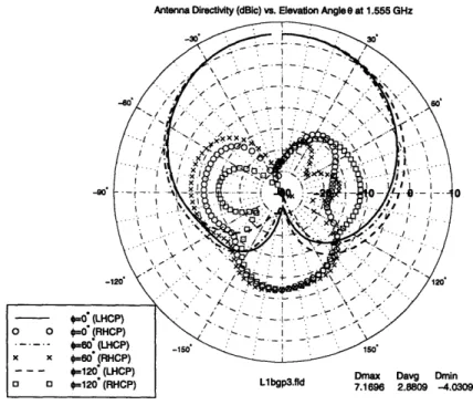
1-4 Radiation Pattern as a function of elevation angle for a typical circular DRA with the two modes excited in quadrature phase ... 18

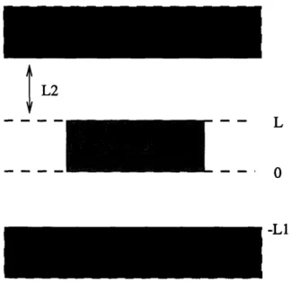
2-1 The DRA is placed at z=O and the boundary condition at z=-L1 and L2 is that of a perfect conductor ... 22

2-2 Top: The Electric Field vector seen from a side view cut for the HE11a mode. Bottom: The Magnetic field vector seen from a cut along the equatorial plane for the HE11, mode ... 27

2-3 Region around and at the DRA is separated into 6 regions ... 28

2-4 Capacitor electric field lines at DC ... 32

2-5 Resonant wavenumber of different modes of an isolated cylindrical dielectric

resonator with relative epsilon = 45. ...

38

2-6

of different modes of an isolated cylindrical dielectric resonator with

3-1 Top: E-field lines at the equatorial plane of the DRA. Bottom: the H-field

3-2 Top: H-field lines at the equatorial plane of the DRA. Bottom: the E-field lines at 0 = 0 for TMo,1. ... 46

3-3 A A/4 transmission line cavity ... 47

3-4 A A/2 transmission line cavity ... 48

3-6 Radiation pattern for Ground plane diameter = 2.96 inch ...

52

3-7 Radiation pattern for Ground plane diameter = 3.7 inch ...

53

3-8 Radiation pattern for Ground plane diameter = 6.06 inch ...

53

3-9 Radiation pattern for Ground plane diameter = 9.16 inch ... 54

3-10 Radiation pattern for Ground plane diameter = 12.28 inch ...

55

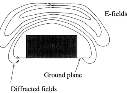
3-11 Electric field lines for the DRA on a finite ground plane for HEll11 mode .. 56

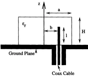
4-1 Geometry of probe-fed cylindrical DRA in the plane containing the axis of

the DRA and the probe ...

60

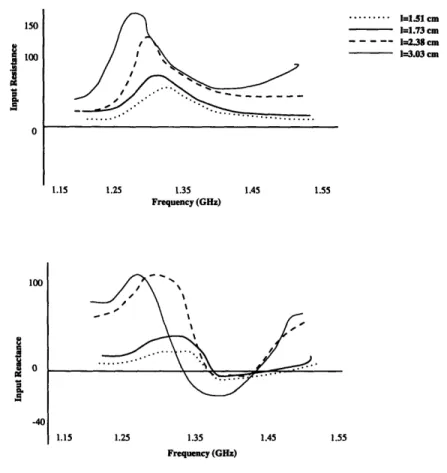
4-2 Input impedance of a dipole as a function of aspect ratio and electrical length 61 4-3 Input impedance of a DRA as a function of probe length, 1 ... 62

4-4 Model for the input impedance ... 63

4-5 Input Impedance as a function of ground plane size ... 64

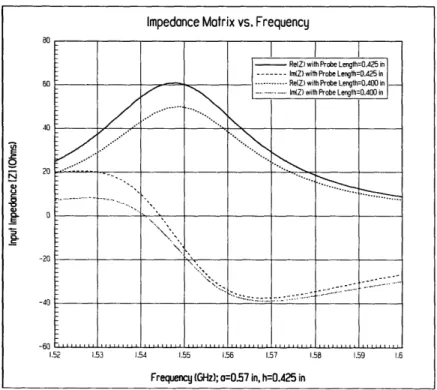
4-6 Input Impedance for a cylindrical DRA with a=0.57in, h=0.425 in and probe length 0.400 inch and 0.425 inch ... 65

5-1 Cylindrical and Ring Resonators . ... 69

5-2 Geometry of the diagonal Slot ... 72

5-3 Input Impedance for W=0.420 in, H=0.425 in, L=0.05 in ... 73

5-4 E-field lines at the equatorial plane of the DRA with rectangular slot. Top:

5-5 Radiation Pattern for W=0.420 in, H=0.425 in, L=0.05 in ... 75

5-6 Input Impedance for W=0.210 in, H=0.425 in, L=0.05 in ... 76

5-7 Input Impedance for W=0.530 in, H=0.425 in, L=0.05 in ... 77

5-8 Input Impedance for W=0.420 in, H=0.425 in, L=0.025 in ... 78

5-9 Input Impedance for W=0.420 in, H=0.425 in, L=0.075 in ... 79

5-10 The different parameter for the case run for L ... 80

5-11 Input Impedance for W=0.420 in, H=0.2125 (lower) in, L=0.05 in ... 80

5-12 Input Impedance for W=0.420 in, H=0.2125 (upper) in, L=0.05 in ... 81

5-14 E-field lines at the equatorial plane of the DRA with rectangular slot. Top: The field lines at 1.575 GHz (lower resonance) Bottom: The field lines at

1.620 GHz (higher resonance) ... 83

5-15 Real part of input impedance for an elliptical DRA with a=0.5 in, b=0.57

5-16 Imaginary part of input impedance for an elliptical DRA with a=0.5 in, b=0.57 in, and h=0.425 in; excited with a monopole of height 0.425 in . . . 85

5-17 Smith chart for S11 for an elliptical DRA with a=0.5 in, b=0.57 in, and h=0.425 in; excited with a monopole of height 0.425 in ... . 86

5-18 Radiation Pattern as a function of elevation angle for an elliptical DRA with a=0.5 in, b=0.57 in, and h=0.425 in; excited with a monopole of height 0.425 in ... 87

5-19 Radiation Pattern as a function of azimuth angle for an elliptical DRA with a=0.5 in, b=0.57 in, and h=0.425 in; excited with a monopole of height 0.425 in ... 87

5-20 Geometry of the Triangular DRA ... 89

5-21 Reflections of the Wave inside a Triangular DRA ... 89

5-22 Input Impedance of the Triangular DRA . ... 90

5-23 Radiation Pattern of the Triangular DRA as a function of elevation angle 91 5-24 Radiation Pattern of the Triangular DRA as a function of azimuth angle .. 91

5-25 Geometry of the Paddle Feed in comparison with the traditional Monopole 92 5-26 Smith Chart showing the reflection coefficient parameter S_{1 1}of the elliptical DRA using a Paddle Feed ... 94

5-27 Radiation Pattern as a function of elevation angle for an elliptical DRA with a=0.5 in, b=0.57 in, and h=0.425 in; excited with a capped probe of height 0.425 in ... 95

5-28 Radiation Pattern as a function of azimuth angle for an elliptical DRA with a=0.5 in, b=0.57 in, and h=0.425 in; excited with a capped probe of height 0.425 in ... ₉₅

5-29 Geometry of the DRA patch antenna ... 97

5-30 Input Impedance of the DRA patch antenna near the resonant frequency for

the patch antenna ...

98

5-31 Input Impedance of the DRA patch antenna near the resonant frequency for

the DRA antenna. . . . ... 99

A-1 Input Impedance for a cylindrical DRA with a=0.57 in, h=0.15 in, 1=0.15

in, Er = 45 . . . . ... ... 104

A-2 Input Impedance for a cylindrical DRA with a=0.57 in, h=0.20 in, 1=0.20

in, Er = 45 . . . . ... ... 105

A-3 Input Impedance for a cylindrical DRA with a=0.57 in, h=0.30 in, 1=0.30

in, Er = 45 . . . ... ... 106

A-4 Input Impedance for a cylindrical DRA with a=0.57 in, h=0.425 in, 1=0.425

in, Er = 45 . . . . . . . ... 107

A-5 Input Impedance for a cylindrical DRA with a=0.57 in, h=0.475 in, 1=0.475

in, Er = 45 . . . ... 108

A-6 Input Impedance for a cylindrical DRA with a=0.57 in, h=1.5 in, 1=1.5 in,

Er = 45 ...

...

.

109

A-7 Input Impedance for a cylindrical DRA with a=0.57 in, h=1.5, 1=0.425 in,

Er = 45 ...

...

.

110

B-1 Input Impedance for a ring resonator for a=0.57 in, b=0.05 in, h=0.425 in,

r = 45 ...

...

. 112

B-2 Input Impedance for a ring resonator for a=0.57 in, b=0.15 in, h=0.425 in,

Er = 45 ...

...

.

113

B-3 Input Impedance for a ring resonator for a=0.57 in, b=0.25 in, h=0.425 in,

Er = 45 ...

...

. 114

B-4 Input Impedance for a ring resonator for a=0.57 in, b=0.3 in, h=0.425 in,

r = 45 ... . 115

B-5 Input Impedance for a ring resonator for a=0.57 in, b=0.35 in, h=0.425 in,

List of Tables

1.1 Salient Features of Modes of a Cylindrical DR ... 15

2.1 Comparison of Resonant Frequency for HEM 1 mode using empirical

for-mula by Mongia and the Magnetic wall model developed in this section. .. 26

2.2 Comparison of Resonant Frequency for HEM1ll mode for a cylindrical

res-onator in free space using empirical formula by Mongia and the magnetic

wall model with the perturbation correction (Perturbation) ...

31

2.3 Value of P for various modes of a cylindrical DR ... 40

2.4 Resonant Frequencies and Q Factors of the Five lowest modes for a cylindrical

DRA with dimensions a=5.25 mm, L=4.6 mm, and er = 38 ...

41

4.1 Input resistance as a function of Aspect Ratio ... 60

4.2 The Resonant Frequency and Input Impedance for various Ground plane sizes 64

5.1 Comparison of Resonant Frequency for HE 11 mode between numerical

sim-ulation by finite elements (FE) and the material perturbation (MP) model

Chapter 1

Introduction

1.1 Background

This thesis is the documentation of the research that was performed on Dielectric Resonator

Antennas when I was at Qualcomm. The significance of this thesis is that it resulted in

some important theoretical models for resonant frequency, radiation, and input impedance. It also gives the design rules for tuning the frequency and the input impedance. In the course of gaining this understanding, several novel radiating elements were invented.

Dielectric Resonator Antennas (DRAs) are ceramic resonators that radiate energy into

space when excited appropriately. Besides applications in antennas, these ceramic

res-onators are used in microwave circuits in areas such as filter and combiner applications. Usually they would be encased in a casing to prevent energy lost through radiation when used as such devices. The figures of merit for these resonators are their Q factor and temperature stability. The Q factor can range from 20 to 50000. The relative dielectric constant (,) for commercially available dielectric resonators (DRs) can range up to about

an cr = 90. The temperature coefficients of resonant frequency (f) can range from about

-6 to 4 ppm/°C. The general characteristics of dielectric resonators were described very

comprehensively by D. Kajfez and P. Guillon [24].

In recent years, DRAs have enjoyed a strong following among antenna engineers. At QUALCOMM, the interests in such antennas are due to its prospect of shrinking down the

sizes of antennas for satellite phone operations and its potential in reducing the cost and

ease of manufacturing. DRAs are one of the most recent progresses in antenna technology, taking its place on par among the more common antennas, such as wire, microstrip, horn,

and reflector antennas. Perhaps, for the reason that it is such a recent development that

there is still much room for development but with very little published material for reference.

The review paper by Mongia and Bhartia [26] is an excellent paper that outlines the major characteristics of the DRA with respect to modes and their respective resonant fre-quencies. The cylindrical DRA is emphasized in their paper. The rectangular and spherical DRAs were also touched on briefly. It is a good place to start. Equations for the resonant frequency and bandwidth of the cylindrical DRA were provided based on empirical formu-las. The drawback is that it was not intended to contain information such as impedance models or radiation on finite ground plane. There was not enough space for them to write everything.

A few weeks after I decided to embark on this subject as my thesis topic, a publication

appeared in the June issue IEEE Magazine entitled, Recent Advances in Dielectric Resonator

Antenna Technology [27]. This is a paper that describes the current DRA technology being

pursued at Communications Research Center in Canada that is done in collaboration with

the Royal Military College of Canada. The technologies being pursued are novel DRA ele-ments for wide-band, compactness, circular polarization, high gain and active applications.

I suspect that they are pursuing DRA array technology. Their paper has an unusually

strong emphasis on couple slot feed, circular polarization (CP) DRA, and arrays.

DRA has the inherent merit of having no metallic loss. This merit is especially good for high frequency applications where conductor loss is proportional to the frequency. The

exploitation of this characteristic is in millimeter wave satellites where they can be used for

satellite to satellite communication. The earth atmosphere is opaque to the electromagnetic

spectrum at millimeter wave due to absorption by 02 and N2 molecules in the atmosphere.

This means that information transmitted from one satellite to another satellite via

mil-limeter wave will have increased security due to the impossibility to tap such signals from

earth.

Another advantage is that because it is usually operated at high permittivity, it allows the antenna to be shrunk in physical dimensions because the wavelength is reduced by

approximately a factor of . DRAs also offer easy coupling schemes to transmission lines

by simply varying the position of the feed points. And there is much room for flexibility in design to optimize for bandwidth. On the manufacturing side, the DRA can be easily tuned to its resonant frequency by using a tuning screw attached above the DRA. The large

degree of freedom means that design is difficult because a lot of variables interplay with each other. However, if the physics is well understood, it is possible to design the DRA to

operate at nearly any rational input impedance, thus eliminating the need of a matching

circuit. The complexity of the DRA can be exploited.

I will now give the outline of what is to come. In the later part of this chapter, I would show some of the salient features of the DRA. In the next chapter, I derived, using the magnetic model, the expressions for the resonance frequency for the cylindrical DRA with

emphasis on the HElls mode. The topic of radiation is discussed next. Its relation to the

multipole expansion of the field distribution is important because it is this relation that

determines the radiation pattern of the DRA. Also important is the discussion on finite

ground plane effects [35], [36], [37], [38], [51]. The equivalence principle formulation [14], [1]

will be used to explain the radiating mechanism. In chapter 4, an impedance model for the

DRA is introduced based on data collected at QUALCOMM and also experimental results

published in [39]. Chapter 5 presents the analysis for the resonant frequency and bandwidth

of the ring resonator. The ring resonator is important because it allows the bandwidth to

be tuned. Some DRA related inventions are also discussed.

1.2 Basic Characteristics

1.2.1 Physical Dimensions and Electrical Properties

Like most good things in life, DRAs can come in many forms of shapes and sizes. The most common shape of the DRA is the cylindrical DRA. This is shaped like a cylinder with its

radius, a, and height, h. It usually has an aspect ratio - the ratio of radius over height (a/h)

- of about 0.5 to 4. The DRA usually sits on top of a ground plane and is excited using

a probe or aperture. The radiation pattern and the feeding method depend on the mode

of interest. The DRA can resonate at many different modes. For the cylindrical DRA, the modes are analyzed and indexed in a similar manner as that of the dielectric waveguide. As

with the dielectric waveguide, the three spatial coordinates are the radius, p, the azimuthal

TI

X

y

P

Figure 1-1: Coordinate System.

1.2.2 Modes

Transverse modes are defined as modes with transverse E or H fields to the z axis. In waveguides, it is advantageous to solve Maxwell's equations by considering the transverse E

and transverse H separately. The axial vector gives all the information needed to calculate

the rest of the vector components. As with the dielectric waveguide, to satisfy the boundary

condition of continuity of tangential fields at the boundary of the dielectric and air, the

only transverse fields that can exist are the modes with no azimuthal variation such as

TEol0 , TEo011+, TMol0 , and TMo011+. All the other modes are hybrid modes just like the

dielectric waveguide [14]. Table 1.1 summarizes some of the major modes that can exist

in a cylindrical DRA. Note that for the cos variation, we could replace it with sin

k

or

a linear sum of both. This is a degeneracy as both the orthogonal modes with cos

and

sin

variations can both simultaneously exist in a DRA with the same frequency. General

]

treatment of modes in cavities and waveguides can be found in electromagnetic textbooks

[7]- [15].

Mode

Plane of Symmetry at z=O

Fields inside Resonator

Far Fields

TEo1a Magnetic Wall H = Jo(hr) cos (z)

E

E,=O0

TE0 11+6 Electric Wall H, = Jo(hr) cos (z) Mag. quadrupole

E,=O0

TMo0 6 Electric Wall

Ez

H,=O

TMo0l+6 Magnetic Wall

Ez

H,=

0

HE1 15 Electric Wall E = J1 (hr) cos (z) cos q5 Mag. dipole

H,-O

HE2 16 Electric Wall Ez = J2(hr) cos (3z) cos 2q Mag. quadrupole

EHl1 1 6 Magnetic Wall H = J1 (hr) cos (3z) cos qS Elec. dipole

E, O

EH21 Magnetic Wall Hz = J2(hr) cos (z) cos 20 Elec. quadrupole

E,-0

Table 1.1: Salient Features of Modes of a Cylindrical DR

1.2.3

Feeding structures

The general feeding mechanism for waveguides and cavities is described in the classic book by Collin [4], [5] and also by Jackson [11]. These feeding structures are usually small electric or magnetic dipoles. The reason for why this is so is because the field distribution for the low order modes when expressed as an expansion in multipole terms would contain strong low order terms such as electric dipole or magnetic dipoles terms. Therefore to couple the energy from the probe into the cavity, electric or magnetic dipole probes are used. To obtain magnetic dipoles, small circular current loops are usually employed. However, in practice, variants of these methods are used. For example, it is more typical to see the DRA being

excited by a short monopole antenna rather than a dipole. Also, a half-circular current loop

is more common in practice.

The apprehension of the appropriate feed mechanism can be obtained in the following way. Firstly, the natural fields in the cavity can be expanded in multipoles. Van Bladel [21], [22] showed that for modes of any shape of the DR are the non confined type. The dominant

is the electric dipole term followed by higher order electric and magnetic multipoles. For resonator shape that is axisymmetric, it can also support confined modes. For confined modes, the electric dipole term contributes dominantly.

Therefore, we can picture that embedded in the DRA are these tiny electric or magnetic dipoles. The exact choice is dependent on which mode we choose to excite. For example,

to excite the HE1 1, mode which radiates like a horizontal magnetic dipole, we can create

an aperture underneath that radiates a magnetic dipole through the surface of the aperture

as shown in Figure 1-2. This is called slot-coupled. We can also use a vertical monopole as shown in Figure 1-3

Coupling Aperture

-- _____________

Microstrip Feed Line

_DRA

Grounded substrate

Monopole feed probe

-

Ground

Plane

Coaxial Cable

Figure 1-3: A DRA fed using a monopole.

1.2.4 Radiation Patterns

From the last section, we know that the fundamental modes of the DRAs radiate like magnetic or electric dipoles. This is because the field distributions in the cavity for the

low order modes support these terms. For radiation study, a natural approach to study

is to expand the radiated fields using the multipole expansion technique. In the multipole

expansion technique, any arbitrary radiation pattern is decomposed into a sum of dipole,

quadrupole and higher order multipole terms. Jackson [11] has a good treatment of this

subject in Chapter 16 of his book.

For low profile antennas operated at low order modes, the contribution from the higher order poles are usually weak. Generally, the smaller the radiating element is compared to the free space wavelength, the better this approximation is. H. A. Bethe [33] has applied this method to the study of radiation from a small aperture in a waveguide.

DRAs can also be used to produce circular polarization [29]. There are actually two

HEll, modes which are orthogonal. Some people prefer to call one of it as odd and the other

as even to distinguish between the two. To obtain CP from HE₁₁s, each of the degenerate

mode must be excited at 900 phase difference. Figure 1-4 shows the radiation from a circular

DRA with dimensions of a=0.57 inch and h=0.425 inch with an

= 45 for the elevation

cut when excited in this fashion. Throughout this thesis, in the polar radiation plots,

Dmax refers to the maximum directivity, Davg refers to the average directivity averaged

from -80

<

< 800 for the major polarization direction (either Right Hand circular

polarized (RHCP) or Left Hand Circular Polarized (LHCP) ) for all 0 and Dmin refers to

the minimum directivity for the major polarization at 0 = 80

As a low profile antenna, the radiation from a DRA is sensitive to the ground plane size. This is discussed in Chapter 3 of this thesis. For finite ground plane sizes with large

Antenna Directivity (dBic) vs. Elevation Angle e at 1.555 GHz

Figure 1-4: Radiation Pattern as a function of elevation angle for a typical circular DRA

with the two modes excited in quadrature phase

diameter (greater than 1 A), geometrical theory of diffraction (GTD) can be used [38], [51]. For consumer applications, a smaller antenna size is desirable and therefore the ground plane is usually designed to be as small as possible. A small sized ground plane of less

than a quarter wavelength can be used with the DRA without significantly distorting the

radiation pattern.

1.3 Method of Analysis

There is no exact analytical solution to the Maxwell's equations for many of the complicated

structures of the dielectric resonators that are used as antennas. In view of this, to attempt

to gain some logical understanding, approximate models must be used to obtain answers in closed form. This is in accordance with the early developments of quantum theory. In the

beginning, when the radiation from the hydrogen atom was not understood, ad hoc methods

such as the Bohr planetary theory of the atom was used to predict the radiation spectra.

Of course, this cannot be correct for reasons of stability, because an electron moving in orbit would be accelerating and would thus radiate energy away and in the end collapse

into the nucleus. The rest is of course history. De Broglie proposed that those atoms were de Broglie waves, and given that they are waves, it was natural for an uncertainty principle

to be formulated and the need for a wave equation to describe the space time variation of

the wave. Thus, Bohr's theory led to new ideas that suggested the existence of the particle

wave duality. Perhaps using a model as ad hoc as it may be might lead to some insights

that were not captured from experience and intuition.

According to my research, the most popular models to analyze these DRAs are the mag-netic wall model, the transmission line model and numerical methods (Method of Moments [18] or Finite Elements[19], [20]). The magnetic wall model and the transmission line model are good for building physical insight. However, they are not as accurate as numerical

meth-ods. Numerical methods are the most accurate but they offer very little physical insight

and a good reliable finite element program may take as long as 6 hours to solve a problem

at a particular frequency. Thus, for anyone wishing to increase the rate of her design cycle,

it is usually good to start off with an analytical model and based on the analytic model

refine her design using numerical methods. For the remaining of the chapters, the magnetic wall model will be used to analyze these DRAs. The predicted results using the model will

then be corrected by analytical means if possible using perturbation theory or correction

factors. Design curves from numerical methods and reported experimental results will also be included.

1.4 Summary

In this chapter, I outlined some salient features of the DRA. Some reasons for using the DRA are its inherent merit of having no metallic loss, small physical size, easily tunable,

and the large degree of design freedom in choosing the parameters. The characteristics

of the major low order modes can be adequately approximated by keeping the low order

terms of the multipole expansion for the field distribution. The radiation pattern of the

DRA would ultimately depend on the field distribution inside the DRA. For example, for

the H 1ll mode, the fields inside the DRA can be approximated closely by a horizontal

magnetic dipole. Therefore the radiation pattern for that DRA at that particular mode will

be that of a horizontal magnetic dipole. Methods of feeding the DRA to excite the mode of interest using monopole probe and slot fed method are also discussed.

Chapter 2

Resonance and Bandwidth

2.1 Introduction

The formulation in terms of TE and TM modes in guided wave theory was motivated by the

observation that the complicated wave problem can be separated into two main problems

of finding the electric and magnetic fields transverse to the direction of propagation. When

these two quantities are found, one could obtain the other components by using Faraday's

Law and Ampere's Law as formulated in Maxwell's equations. The fields in a resonator

are standing wave fields and thus the problem can be solved by assuming that the waves

are guided waves propagating in +z and -z directions. To find the transverse components

the following equations called homogeneous Helmholtz equations are solved where z is the

direction of propagation:

[V2+ w2pe]Ez = 0

for transverse magnetic (TM) case and,

[V2 + w2pE]Hz = 0

for transverse electric (TE) case.

The other field components are given by Faraday's and Ampere's laws after doing some algebraic manipulation to solve for each vector components in terms of Ez and Hz. The final field expressions are given as:

E,

k _ [v. s-E + iwfV

x Hz]

1 [s

H,

=

k2 _

[V, --H -

iwpV

x E]

where k = w2pe is the wave number and s is the transverse components. I am using the

same notation that was used by Kong [14]. In the case of cylindrical dielectric resonators,

the equations are expanded in cylindrical coordinates and substitution Hz = 0 for the TM

case into the above equations give:

Ep = k2 _ k2 [ p Ez (2.1)

1 1 (2.2)

Hp = k2

_ k

H = k

_k

[iwe

a

Ez]

(2.4)

2.2 Formulation of the Cylindrical Dielectric Resonator

us-ing the Magnetic Wall Model

The physical dimensions and coordinate origin is as shown in figure 1-1 and 2-1. The

height of the resonator is L and the boundary condition at z=-L1 and Z=L2 is that of a

perfect conductor. For the HEll1 mode, Hz 0 so we will solve the problem for the TM

case. The field within the region 0 < z < L is,

E = J (kpp)cosq(Aeiz

+ Be

Z)

where p is the propagation constant in z direction. Knowing Ez we can find the other

field components by using equations (2.1) to (2.4). We get,

IL2

L

A

-L1

Figure 2-1: The DRA is placed at z=O and the boundary condition at z=-L1 and L2 is that

of a perfect conductor

(2.6)

(2.7)

E = I32)

[JI (kpp) sin (Aeiz - Be-iZ)]

iwe

H = p(k2 2) -[Ji(kpp) sin (AeiP + Be-iPZ)]

H

=

k2

[(kpJo(kp)

-

Jl(kpp))cos (AeiZ +Be-iIZ)]

V - p2 P (2.8)

where

k2 = 2

t

kp and P3

are the propagation constants in p and z respectively. The radial propagation

constant k can be obtained by using the condition that H is zero at p = a. This is due to the perfect magnetic conductor assumption at the curved surface. This condition yields

kpaJo(kpa)

=

J(kpa)

This gives kpa = 0, 1.85, 5.3, ....

Figure 2-1 shows the segmentation of the region around the DRA. Let region 1 be the

region where -L1 < z < O0. The Ez field here is,

Ezl = J (kpp) cos b(CeQ z + De- al z)

L

- -

-Similarly, the fields in region -L1 < z < 0 are:

a, 1 Z)

Ep=i

k2

-a

[kpJo(kpp)

-

Jl(kpp)] cos O(Ce

lz - De

)

(2.10)

E1

p(k

_ Jl(kpp) sin

q(CelZ

- DeZ)

(2.11)

iwo

Hpl

p(k

_

a2

J

(k

) sin b(Ce

z + De

lZ)

(2.12)

iwo 1

=

+

-

c2

[(kpJo(kpp)-J(kpp))(Celz + De-al) cos]

(2.13)

where al is the wave propagation constant in region 1.

The field E¢,1 must vanish at z = -L1 because of the conducting wall. This results in

D

= Ce

_L1

Therefore the above equations can be rewritten in terms of one unknown, C, as

2Cae-aL1 1

Ep1=

k

_-a

_[kpJo(kpp)

_-

_{Ji(kp)]cossinh(al(z}

_{+ L1))}

_(2.14)

--2Cale-aL1

E0

=

Jl(kpp)sinqksinh(a(z

))

(2.15)

Ez

= 2CJ1(kpp) cosqcosh (a(z + L

))

(2.16)

2Ce-a

iweo

Hp = 2Cep(k

-aL)

J (kpp) sin k cosh (a (z + L1))

(2.17)

2CiwEoe -L1 1

Ho1

C=

i°e

[kpJ(kpp)- -Jl(kpp)]cosh (al(z + L)) cosq$

(2.18)

In an analogous manner, by making the substitution -L

= L

+ L, we obtain the

following fields for region 2:

2Fa2 ea2(L2±L) 1

Ep2 = k2 _2

[kpJo(kp)

J(kpp)]

q sinh

L

L))

(2.19)

-2Fa2 e2 (L2+

E02

=

p(k2 _a2)

J(kpp) sinq0sinh

(a2(z - L

-

L))

(2.20)

Ez2 =

2FJ

(kpp)

0

L))

H

2Fa

e

J (kpp) sin 4cosh (a

(z -

L))

(2.22)

2kpe(

a1

L+

)(kpp)]

[J(kp)-

cosh (2()

F k2 [J

(kp)

q(2.23)

where

a2 = k2 k22 (2.24)

Next, we use the boundary condition at z=0. The boundary condition is that the

tangential fields must be continuous. This lead to the following condition,

E01

-if(Aeifz - Be-ifZ)

Hp(Ae + Be

E(AePz

+ Be-ifz)

=

E2

=

-2Cale

L1

sinh

(al (z +

L1))

= Hp2

= 2coCe-, Li cosh

(al

Dividing the equation 2.26 by equation 2.28, we get

(Aeiz

-

Be-if z)

ip(Aeiz + Beifz)

= alE, tanh (al (z + L1))

Now, we must remember to evaluate z at 0. Doing so we get from equation 2.29

(A - B)

if] (A -- B)

lEr tanh (ilL1)

(A + B)

The boundary condition at z=L is the same as at z=0. Thus we just need to substitute

the variable L1 with -L - L2 and evaluate z at L. Doing so we get,

(Aei#L - Be-iPL)

iP

(Ae

+

Be-ifL)

tanh

)

Now, for a perfect standing wave, A and B must have the same amplitude. Thus

B

- = e

A

With this, we can evaluate the left hand side terms

and

(2.25) (2.26)

(2.27) (2.28)

A-B

= -i tan 0/2

A+B

and

Ae

i tan (L - 0/2)

Aei

+ Be-i3

02

= arctan( _

tanh(aL1i))

(2.32)

= arctan ( 13 tanh (-a

L

))

(2.33)

2 P

For an isolated DRA in free space, we let L1 and L2 approach oo. Then the above

conditions reduce to,

2=

-

= arctan(

)

(2.34)

02 _ 2 Er

= arctan (

)

(2.35)

2

In free space with e1 1, 2 = 1, and al = a2 we have,

O1 02 a6r

L =- + - = 2 arctan (

(2.36)

2 2

where a2 is given by equation 2.24 and P is given by equation 2.9, both which are the

z-propagation constants in the respective dielectric permitivities.

Now, we have the resonant frequencies for the HEll5 by applying equation 2.36.

2.2.1

Summary and physical interpretation

We attempted to solve the problem of an isolated DR in free space by using a simplified model. In this model, we assumed that the curved surface of the DR is a perfect magnetic conductor. When an EM wave propagates from region of high permittivity to low

What is the motivation of this concept?

Now, we know that the intrinsic impedance is inversely proportional to /.

Thus, in

region of high permittivity, the impedance is very low. In transmission line theory, the

reflection coefficient is given by RL- . For a wave traveling from high to low region of

permittivity, Ro is much smaller than RL. Thus, the reflection coefficient approaches 1.

This is an open circuit thus we can assume it to be a perfect magnetic conductor. On the

other hand, for a wave traveling from region of low permittivity to high permittivity, R is

much larger than RL. Thus the reflection coefficient approaches -1. This is a short circuit

in transmission line, or a perfect electric conductor.

Therefore with a curved surface as a perfect magnetic conductor and the ends as perfect

electric conductor at some distance away from the resonator, we derived the dispersion

relations. This allows us to find the resonant frequency of the DR.

Mongia and Bartha [26] have an empirical expression for the calculating the resonant frequency for the HEM116 mode. Table 2.1 compares the values obtained using the method developed in this section with their formula for a cylindrical dielectric resonator in freespace.

Table 2.1: Comparison of Resonant Frequency for HEM1 1 6 mode using empirical formula

by Mongia and the Magnetic wall model developed in this section.

Ier radius (in) height (in) Mongia (GHz) Magnetic Wall (GHz) Error

45

0.57

0.300

1.92

1.56

19

45

0.57

0.425

1.58

1.30

18

45

0.57

0.800

1.22

1.05

14

45

0.57

1.500

1.03

0.95

8

45

0.40

0.300

2.25

1.58

18

30

0.57

0.425

1.92

1.58

18

The error between the magnetic wall model and the formula obtained by Mongia is large. The reason is because the magnetic wall model is not a perfect model. The dielectric

resonator is not a perfect magnetic conductor, but fields actually penetrate across the curved

surface of the resonator.

Figure 2-2 shows the plots of the electric field vector for the HE11l mode. The top

figure is the electric field plot on the side of the resonator. The lower figure is the cut along

the equatorial plane. From both sketches, we can deduce that the dominant multipole

expansion term should be the horizontal magnetic dipole term.

E

H

Iv

I

!

Figure 2-2: Top: The Electric Field vector seen from a side view cut for the HE1ll mode.

Bottom: The Magnetic field vector seen from a cut along the equatorial plane for the HEl11

mode.

2.2.2

Perturbation Correction to the Magnetic Wall Model

The previous model gave a close answer but we can get a more accurate result by including a perturbation model. We know that the magnetic field does penetrate through the surface of the DR because it is not a perfect magnetic conductor. So let's move the perfect magnetic conductor out to a radius distance of oo. What is the new resonant frequency? We will solve this using the perturbation model.

From cavity theory, when an outward perturbation is made at a place of large magnetic field, the resonant frequency is lowered; if made at a place of large electric field, the resonant

frequency is raised. The opposite effect occurs for an inward perturbation [14].

Let us collect our results so far, in region 0 < z < L which I will label as region 6 using

equations 2.5 to 2.8 after substituting the appropriate constants for A and B,

E06

(2.37) (2.38)

= B° [kpJo(kpp)

-

Jl(kpp)] cos sin (z - 0)

iw= o p 2

01

Ez

=

J1(kpp)coskcos(z-

-2)

Hp

=

-EoJ1

sin cos (,z -

)

P 1 1

H0

=

--

,Eo[(kpJo(kp)-- .

(kpp))cos

cos(3z-

-)]

2~~~~ (2.39) (2.40) (2.41) where -iweo

-Eo

2

₎

Now, let us break the region into 6 different regions as shown in the Figure 2-3. The region with the DR is region 6, and each corresponding region's fields will be subscripted with the region number. To use the perturbation model, we must first calculate all the fields in each region because we need to eventually calculate the energy.

i

5

3 :

2

4

Figure 2-3: Region around and at the DRA is separated into 6 regions

For region -L1 < z < 0, using results from previous section, we can immediately write

down the fields ensuring continuity at boundary as,

Eo=

3 sin -1

1

=

sin

iwo sinhClL1

P

Eo/3 sink

E01 =

s

Jl(kpp) sin 0 sinh (al(z + L1))

(2.43)

piweo sinhaIL 1 COs

Ezl

cosh

Jl(kpp) cos cosh (al(z + L1))

(2.44)

cosh a, L1

1 cos

'-Hp

_{pcosha L}

cos

H,1 = -ErEoc

_coshalL

[kpJo(kpp)- -Jl(kpp)]coscosh(al(z

+ L1))

(2.46)

1

p

and similarly for region L < z < L2,

Esin (L - ~)

Ep2

=

Eo72ie

[kJo (kp)

-

Jl(kpp)] cos

sinh

(a

(z - L

- L)2.47)

2L2) p

E

sin (3L - -)

2

iwEo

(kpp)

4

p iwEo

sinh (-a

L

)

cos (fL -

-)

E.z2 =2

_cosh(-a

JI(kpp)

cos cosh (a2(z - L

- L))

(2.49)

2

L

)

=rEo

Hp2

) J (kpp) sin bcosh (a2(z - L

-

L))

(2.50)

p

cosh

(-a

L

)

co (L -

)

H2

-ErEo

(-

)[kp J(kpp)

-

J (kpp)] cos

q

cosh (a2(z - L

- L))(2.51)

The fields in regions 3, 4, and 5 are now selected such that the solutions are of the forms of modified Hankel functions which are monotonically decaying with increasing p. Thus,

the fields in region 3, 4 and 5 are: In region 3:

E03 =

-Eo

sin(

)JK(kpa)

(kp2p)

sin

0

sinh

(al(z + L))

(2.52)

E 3 = COS( K1

(kp2p)

(a

cosh (alL1 )Kl(kp

a)

co - J (k a)

Hp3 =

-erEo

co

p

Kl(kp2p) sinqbcosh (al(z + L1))

(2.54)

p cosh (alL )K(kp2 a)

In region 4:

E04 = -Eo la J( (kpa) sin (2.55)

Ez4

=

( )

K (kp2p)

cos cos (z -

1

K1(Ikp2a) 2

Hp4 =

-EEO

J(ka)

pK1

In region 5:

E05 = -E₀

if3

(kpa)

(kp2p)

0

(

(z

L))

(2.58)

wEo

psinh (-a

L

)Ki (kp2a)

cos (L

-

B-)J(k a)

Ez

cos

(L-

)J(kpa)

Kl(kp2p)

cos cosh (a2(Z - L2 -

L))

(2.59)

cosh (-a2L2)K (kp2a)

Hp5 = EE cos

(

(ka)

p

a)

where

k2 = 2 _ k2

Now, we have all the field expressions from region 1 to 6. We can proceed to apply perturbation theory to the problem. We can use the expression given in [14]:

AWm- AWe

w = o(l

Wm- We

_(2.61)

where wo is the original frequency obtained using the Magnetic Wall model from the

previous section. lAWm and AWe are just the energies in regions 3, 4, and 5.

Written in a different form,

Wm3 + Wm4 + Wm5 - We₃ - We4 - We5)

W( + Wm1 2+ Wm6 + Wel + We2 + We6

where

Wmi =

J

fvidV(plHo

(2.63)

Wei =

Jvi

where Eo and Ho are the fields in the region where the fields in region i. Again, we compare the results to the empirical formulas obtained by Mongia. The values are shown

in the table below.

Table 2.2: Comparison of Resonant Frequency for HEM1 1

l

in free space using empirical formula by Mongia and the magnetic wall model with the

perturbation correction (Perturbation).

IEr radius (in) height (in) Mongia (GHz) Perturbation (GHz) Error

45

0.57

0.3

1.92

1.90

1.1

45

0.57

0.425

1.58

1.61

1.6

45

0.57

0.8

1.22

1.27

4.1

45

0.57

1.5

1.03

1.09

5.8

45

0.4

0.3

2.25

2.27

0.9

30

0.57

0.425

1.92

1.95

1.6

because the magnetic field does penetrates across the walls of the DR. Thus, we perturbed our solution by moving the magnetic walls outwards. According to perturbation theory, depending on whether there is an increase in magnetic or electric energy, the resonant frequency would shift either up or down.

The physical interpretation of the perturbation result is in order. This is how I

under-stand it qualitatively. First, our unperturbed system is at resonance. At resonance, the

time averaged electric and magnetic field energies are equal. If you perturbed the system such that you take away from it equal quantities of time averaged electric and magnetic

field energies, then the system is still at resonance because those two quantities are still

equal.

Next, perturb the system again so that you take away more time averaged magnetic power than the time averaged electric power . The system is now not in balance. There is more time averaged electric field energy than the time averaged magnetic field energy.

Then, the resonant frequency must change to a new frequency such that the total time

averaged electric and magnetic field energy would be equal again. Here is another look at a thought experiment.

Imagine that we have a capacitor. At DC, the electric fields would be non time varying and the field arrows would point from the positive plate to the negative plate as shown in figure 2-4. The energy stored is purely electrical. The polarity of the terminals is now switched. If we change it slowly, the fields would point downwards when the polarity is switched - always pointing from the more positively charged plate to the negatively charged plate. Now, let us change the polarity of the plates at a faster rate. As we increase this

frequency, magnetic fields begin to appear in the space between the plates. This is due to

Ampere's Law. A time varying electric field produces magnetic field. Now, we have some magnetic energy. So, what began as a capacitor is now behaving more like an inductor.

Figure 2-4: Capacitor electric field lines at DC.

Let us increase the rate of change even faster. Now, more and more magnetic energy

builds up. There would be an interplay between Faraday's law and Ampere's law. The time

varying magnetic field would create electric field, and the time varying electric field would create a time varying magnetic field. Soon, the amount of time averaged electrical energy and magnetic energy within the space between the two plates would be equal. Our system

would then be at resonance. And at this point, we can place ,at locations where the fields

are null, conductors so that our original capacitor now becomes a cavity.

Perturb the system now by taking away some magnetic energy. After perturbation, there is more electrical energy than there is magnetic energy. To keep both the energy in balance again, we must increase the frequency to generate more magnetic field. This is

what is described by the theory.

In the same way, we could describe the thought experiment with an inductor in which

case, the result would be the opposite.

2.3 A note on fine tuning

Any derived empirical formula is not expected to be exactly precise. The derived formula

errors and many other sources. The antenna engineer must therefore understand the

un-derlying physics to know which parameter is to be reduced or increased to fine tune the

resonant frequency of the antenna.

Even if the antenna engineers fully understand the underlying physics, as the antenna

gets manufactured, manufacturing tolerances on design parameters will change the resonant frequency. Examples of such manufacturing tolerances are the radome thickness, and the

measurement tolerances for cutting and shaping the antennas.

One must therefore perform a sensitivity and manufacturing tolerance study. I like to

present here a method that can be used to solve this problem. The problem to solve is

the problem of fine tuning the resonant frequency of the cylindrical DRA and to determine

its manufacturing tolerances. It is based on a Taylor Series approximation. The idea is

that manufacturing tolerances are expected to be small changes in the design parameters. Therefore a first order Taylor Series approximation about the difference between the man-ufacturing sample and the ideal sample should be adequate to describe its effect on the resonant frequency.

Let the resonant frequency be a function of the radius a, height L and permittivity er

or f(a,L,Er).

Then, the differential change in the resonant frequency is,

df =

f

da

+

f

db

+

f

d

Making a 1st order Taylor Series approximation,

Afa+f

Ab

Of A

Af = af

Aa + -afAb

+ af

Ar

(2.65)

The goal now is to determine the value of the partial derivatives given by the above equation. At simulation stage, this can be easily done. For example, set Ab = Ae, = 0.

Then vary a by a small amount, Aa. Run the simulation and obtain Af from the simulation.

The value of -9 is then given by Af/Aa. The process can be repeated for the other partial

derivatives. The end result is that the above equation is now a design equation. It tells the designer exactly how much he or she needs to vary the parameters to further fine tune the resonant frequency.

be held constant. This does not present any problem in my formulation. Each of the

change in the parameter can be measured. The change in the resonant frequency can

also be measured. From one manufacturing sample, one would be able to rewrite the

above equation as an equation in n number of unknowns for n number of parameters that

are subjected to manufacturing tolerances. Then one needs n manufacturing samples to

produce n independent equations. The set of n equations in n unknowns are a set of linear

equations and they can be conveniently solved using linear algebra techniques where the set

of equations are expressed in the form Ax = b. If there are more samples than the number

of parameters, then this becomes an over determined system in which the solution can be

obtained by using least squares. The linear algebraic method solution to least squares is also

very straightforward. It is given by ATAx = ATb. The method can of course be generalized

to any arbitrary number of parameters.

This method is so general that it does not even require any understanding of the

un-derlying physics beyond the functional dependence of the resonant frequency. It is also applicable to all forms of manufacturing processes beyond antenna engineering. I believe that this is the power of a Taylor Series approximation. Newton was able to come up with

F = ma - an equation still used today despite lacking a true picture of the actual structure

of space-time. His famous equation was so accurate for describing macroscopic motions because it is a first order approximation in v/c where v is velocity of some object and c is the speed of light.

2.4 Degeneracy and its similarities to the Zeeman effect

-Symmetry

From the field expressions in the DRA, we had a choice of replacing the azimuthal term

cos with sin and vice versa or the linear sum of both and the equations would still

be a solution to Maxwell's equation. Thus, at the same frequency, there are actually two

orthogonal modes that exist for the HE

l mode. What is the source of this degeneracy?

Degeneracy in atomic radiation is a very important subject in Quantum Mechanics.

Many of the physics of degeneracy between antenna radiation and atomic radiation share

the same explanations. I like to discuss this degeneracy in a more broader setting to

understanding of the same phenomena from other areas (Quantum Mechanics).

In the hydrogen atom, which consist of just a proton and an electron, degeneracy is

caused by the symmetry of the system. The Schroedinger equation, which is also a statement of conservation of energy, would contain a term involving the potential energy of the electron which is a function of the distance away from the nucleus, r. The other spatial variables, the

polar angle 0 and the azimuthal angle do not come into play at first order. The quantum

states of the different angular momentum of the electron are orthogonal states. However,

they all have the same energy. So we identify the system as having degeneracy because the energy levels of the different electrons are all at the same level.

Symmetry is also the reason for the existence of degenerate modes in the cylindrical

DRA. The DRA is symmetric in the azimuthal direction. There isn't any azimuthal angle

that is preferred. We could place our probe at any azimuthal angle and all the results would

still be the same had we placed the probe at some other azimuthal angle. But once we have

decided on the azimuthal angle to place our first probe, that would destroy the symmetry

and the other degenerate mode would have to be excited by a probe placed at 900 away

from the probe. This would then be the only other orthogonal mode at the same frequency.

The detection of degenerate energies and its related experiment in Quantum Physics

comes under the name of the Zeeman effect. In the Zeeman effect, magnetic fields are applied

that effectively breaks the symmetry of the system. The application of the magnetic field

interacts with the angular momentum of the electron. Depending on the quantum number of

the angular momentum, electrons at different angular momentum states which all previously

share the same energy will now have different energy levels. The degeneracy is broken. With the degeneracy broken, two or more slightly different frequencies are radiated and it can

be measured. Circular polarized radiation can be observed in Zeeman's experiment. The

interested reader can read more in [2].

We can do an analogy of the Zeeman effect on the DRA. In Chapter 5, I will show

several methods that can be used to break this degeneracy which are simpler to implement.