The East Greenland Coastal Current:
its structure, variability, and large-scale impact
by
David A. Sutherland
B.A., University of North Carolina, Wilmington, 2001
Submitted in partial fulfillment of the requirements for the degree of Doctor of Philosophy
at the
MASSACHUSETTS INSTITUTE OF TECHNOLOGY and the
WOODS HOLE OCEANOGRAPHIC INSTITUTION February 2008
©2008 David A. Sutherland. All rights reserved.
The author hereby grants to MIT and WHOI permission to reproduce and to distribute publicly paper and electronic copies of this thesis document in whole or in part in any
medium nnw nn•mim -.--- r created.
A uthor...
...
... ...
.. ...
...
Joint Program in Oceanography / Applied Ocean Science and Engineering Massachusetts Institute of Technology and Woods Hole Oceanographic Institution January 2, 2008 Certified by.. ... Robert S. Pickart Thesis Supervisor Accepted by... OF TEOHNOLOGY
APR 2 3 2008
LIBRARIES
4/1 Raffaele FerrariChair, Joint Committee for Physical Oceanography
The East Greenland Coastal Current: its structure,
variability, and large-scale impact
by David A. Sutherland
Submitted to the Joint Program in Physical Oceanography on January 2, 2008 in partial fulfillment for the requirements of degree of Doctor of Philosophy
Abstract
The subtidal circulation of the southeast Greenland shelf is described using a set of high-resolution hydrographic and velocity transects occupied in summer 2004. The main feature present is the East Greenland Coastal Current (EGCC), a low-salinity, high-velocity jet with a wedge-shaped hydrographic structure characteristic of other surface buoyancy-driven currents. The EGCC was observed along the entire Greenland shelf south of Denmark Strait, while the transect north of the strait showed only a weak shelf flow. This observation, combined with evidence from chemical tracer measurements that imply the EGCC contains a significant Pacific Water signal, suggests that the EGCC is an inner branch of the polar-origin East Greenland Current (EGC). A set of idealized laboratory experiments on the interaction of a buoyant current with a submarine canyon also supported this hypothesis, showing that for the observed range of oceanic parameters, a buoyant current such as the EGC could exhibit both flow across the canyon mouth or into the canyon itself, setting the stage for EGCC formation. Repeat sections occupied at Cape Farewell between 1997 and 2004 show that the alongshelf wind stress can also have a strong influence on the structure and strength of the EGCC and EGC on timescales of 2-3 days. Accounting for the wind-induced effects, the volume transport of the combined EGC/EGCC system is found to be roughly constant (-2 Sv) over the study domain, from 68*N to Cape Farewell near 60°N. The corresponding freshwater transport increases by roughly 60% over this distance (59 to 96 mSv, referenced to a salinity of 34.8). This trend is explained by constructing a simple freshwater budget of the EGCC/EGC system that accounts for meltwater runoff, melting sea-ice and icebergs, and net precipitation minus evaporation. Variability on interannual timescales is examined by calculating the Pacific Water content in the EGC/EGCC from 1984-2004 in the vicinity of Denmark Strait. The PW content is found to correlate significantly with the Arctic Oscillation index, lagged by 9 years, suggesting that the Arctic Ocean circulation patterns bring varying amounts of Pacific Water to the North Atlantic via the EGC/EGCC.
Thesis Supervisor: Robert S. Pickart Title: Senior Scientist, WHOI
Acknowledgments
This thesis is dedicated to my family, who have supported all my adventures, even as a Yankee, with gusto.
My advisor, Bob Pickart, deserves a huge thank you for giving me the opportunity to pursue this research by inviting me along on the initial cruise and allowing me first crack at the dataset that emerged. He also provided constant guidance and was quick to refocus my attention when it wandered. Funding for the cruise and analysis was provided by the National Science Foundation, under grant OCE-0450658. The WHOI Academic Programs Office and the MIT Assistance Fund also contributed some funds for my travels to present this research at meetings, and for trips to meet with Bob during his sabbatical in Fairbanks, Alaska.
Many others contributed to the processing of the data used here, in particular I would like to thank Dan Torres (ADCP man), Terry McKee, Paula Fratantoni, and Jane Eert. The captain and crew of the RRS James Clark Ross contributed flawless service in obtaining the data during the summer of 2004. Chemical analyses were done by Kumiko Azetsu-Scott and her group at BIO, while Peter Jones, also at BIO, was extremely helpful in his comments on the nutrient chapter.
I would also like to thank the rest of my committee for their encouragement along the way, as well as their open door policy outside of committee meetings. Claudia Cenedese helped immensely with the setup of the laboratory experiments and gave me guidance early on in my grad school career as my initial advisor. Fiamma Straneo also was always ready to give advice, as was Steve Lentz. Dave Fratantoni and Amy Bower invited me on their field expeditions during my time at WHOI, and I will always be ready in case they need more help, as they were great experiences!
My friends in the Joint Program were essential in getting me to the finish line. In fact, I may have faltered at the starting line if it wasn't for the big group we had up at MIT during those first two years: Matt, Max, Ariane, Yohai, Dave, Asher, and Greg. And to all the other students who came in with us and enjoyed those stormy days on the SSV
Corwith Cramer, the Barn, and the Hole in general: thank you!
Along the way many of these same friends actually gave me good scientific advice as well. And my gratitude goes out to past and present office mates and friends, as they provided easy examples to follow, as well as many fun times: Melanie, Jim, Carlos, Andrew, Jake, Bea, Stephanie, Kjetil, and Alex.
And lastly, I would like to express my sincere thanks to the Joint Program for pushing interdisciplinary science, as it led me to meet my future wife! My love for Kelly grew during the years I spent in Woods Hole and without her, my time here would have been vastly different. Thank you Kelly for giving me your love and for always being there no matter what.
Contents
1 Introduction
9
1.1 Thesis outline ... 10
1.2 Background... 12
1.3 Data ... 19
2 Hydrographic and velocity structure of the EGCC
20
2.1 Introduction ... 202.2 Data and methods ... 21
2.2.1 Hydrographic data processing ... 22
2.2.2 Velocity data processing ... 23
2.3 EGCC Hydrographic and velocity structure ... 24
2.3.1 Defining the EGCC ... 26
2.3.2 Section 1 - Cape Farewell (60°N) ... 27
2.3.3 Section 2 -near 630N ... ... ... 30
2.3.4 Section 3 - near 65N ... 32
2.3.5 Section 4- near 66°N ... 34
2.3.6 Section 5 -north of Denmark Strait (680N) ... 36
2.4 Sources of variability in the EGCC ... 39
2.4.1 Dynamical scales of the coastal current ... 39
2.4.2 W ind forcing... 47
2.4.3 Internal variability... 51
3 The volume and freshwater transports of the EGCC
59
3.1 Introduction ... 59
3.2 Transports... 60
3.2.1 Volum e fluxes ... 60
3.2.2 Freshwater fluxes ... 64
3.2.3 Adjusted alongstream transport trends for the EGC/EGCC ... 66
3.3 Simple freshwater budget for the EGC/EGCC ... 68
3.4 Discussion and summary ... 72
4 The freshwater composition of the EGCC
74
4.1 Introduction ... 744.2 Dataand methods ... 77
4.2.1 Analysis methods ... 79
4.3 Freshwater composition of the EGCC ... 85
4.3.1 Pacific W ater ... 85
4.3.2 Sea Ice M elt ... 89
4.3.3 Meteoric W ater ... 92
4.3.4 Uncertainties ... 94
4.4 Interannual variability in the Pacific Water signal ... 97
4.4.1 Calculation of the Pacific Water signal ... 99
4.4.2 Link to the Arctic Oscillation ... 105
4.5 Discussion and summary ... 108
5
Laboratory experiments on the interaction of a buoyant coastal
current with a canyon: application to the EGCC
111
5.1 Introduction... 1115.2 Experimental methods ... 116
5.2.1 Laboratory set-up ... ... 116
5.3 Buoyant current scaling and theory ... 121
5.3.1 Review of scaling for a buoyant current on a slope ... 121
5.3.2 Review of buoyant current separation scaling ... 123
5.4 Results... ... 125
5.4.1 Overview of the steady circulation: 3 cases ... 128
5.4.2 What controls the separation process? ... . . . 132
5.5 Discussion ... .... 136
5.5.1 Oceanographic relevance ... 138
5.6 Summary ... 141
6 Conclusions
144
6.1 Summary of the thesis... 1446.2 Discussion ... .... 146
6.3 Ideas for future work ... 149
A
-
Error estimates for volume and freshwater transports
152
Chapter 1
Introduction
Historically, the subpolar gyre of the North Atlantic Ocean is second only to its southern counterpart, the North Atlantic subtropical gyre and the Gulf Stream, in the amount of observational and theoretical study invested in trying to understand its motions. A general sense of the large-scale cyclonic circulation in the northern North Atlantic, and the
convergence of polar-origin waters with those of the warmer and saltier subtropical region, has been known for at least 150 years, starting with the mid-nineteenth century Danish explorations into the region [see Pickart et al., 2005 for a summary].
However, the details of the subpolar gyre circulation are still lacking, particularly along the boundaries of Greenland, where observations are difficult to obtain due to the presence of sea ice during most of the year that limits the use of research vessels, drifters, and standard mooring designs in the region. Cloud cover consistently blankets the region as well, which inhibits the use of remote-sensing techniques.
The main goal of this thesis is to improve our understanding of the circulation over the shelf region of southeast Greenland, where little is known inshore of the shelfbreak where the main currents of the subpolar gyre reside. The shelf and overlying ocean environment are complex, with numerous bathymetric irregularities, strong wind
forcing on small spatial scales, and multiple sources of buoyancy input (meltwater runoff, precipitation, ice melt), along with intense mixing associated with the frontal region between the polar-origin shelf water and the northern remnants of the Gulf Stream.
Despite these complexities, a coherent coastal current feature has been observed several times near the southern tip of Greenland at Cape Farewell and has been named the East Greenland Coastal Current (EGCC), to distinguish it from the shelfbreak flow of
the East Greenland and Irminger Currents (EGC, IC, respectively). The main objectives of this thesis focus on the coastal current flow and are, specifically, to
* describe the basic hydrographic and velocity structure of the EGCC, both across-shelf and along-across-shelf,
* determine the impact of the EGCC on the regional volume and freshwater budgets of the subpolar gyre,
* identify the contributions of freshwater to the EGCC in order to understand its origins,
* understand the formation process of the EGCC and determine its interaction, if any, with the EGC/IC system at the shelfbreak,
* and place the EGCC in context with other high-latitude coastal currents and understand the dominant processes controlling its behavior.
1.1 Thesis outline
The rest of this thesis is devoted to meeting the above objectives, and to answering any corresponding questions stemming from the research. The chapters are organized as
follows.
Chapter 1 is an introductory chapter, starting with a list of thesis objectives and a brief outline of the thesis. Background on important aspects of the circulation in the subpolar gyre is given next, including some of the main forces that drive it. This broad introduction to the subpolar gyre circulation leads into a more detailed background on what is known about the EGCC from previous studies. Then, the main source of data used in this thesis is introduced along with the motivation for the field project that
produced the data. Details on data processing and additional data sources are left for subsequent chapters.
Chapter 2 describes the hydrographic and velocity structure of the EGCC using sections obtained in the summer of 2004, addressing both the across-shelf and along-shelf evolution of the current. This chapter includes an objective definition of the EGCC, distinguishing it from the EGC, which has been a source of confusion historically. Despite the spatial distinction between the currents, though, the hydrographic properties of the EGCC suggest a close link between the EGCC and the EGC. Chapter 2 concludes with a discussion of additional hydrographic and velocity transects across the shelf at Cape Farewell that begin to elucidate the temporal variability of the EGCC and the main factor, along-shelf wind forcing, that is responsible for this variability.
Chapter 3 continues the description of the EGCC along the southeast coast of Greenland by calculating its volume and freshwater fluxes. These are compared with the calculated transports of the EGC, and are found to be similar in magnitude and co-varying, suggesting that the EGC and EGCC comprise a single system of equatorward-traveling polar-origin water over the Greenland shelf. A simple technique for adjusting the transports to reflect the along-shelf wind forcing is presented, which significantly
enhances the interpretation of the results. Once these adjusted trends are computed, the chapter ends with a freshwater budget calculation for the southeast Greenland shelf region, showing that after the advection of freshwater in the EGC/EGCC system, melt
from sea ice is the next largest contribution.
Chapter 4 utilizes chemical tracer techniques to explore the freshwater
composition of the EGCC in more detail. Specifically, a combination of nitrate-phosphate relationships, oxygen isotope, and alkalinity data are used to quantify the amount of Pacific Water (which must ultimately be of Arctic-origin), sea ice melt, and meteoric water in the EGCC. A discussion follows on the origins of the EGCC, concluding that it does contain a significant amount of Pacific Water and thus is linked to the EGC as it exits the Arctic Ocean at Fram Strait. Historical data are then used to look at the interannual variability in the Pacific Water signal in the EGC/EGCC at Denmark and
Fram Straits (see Fig. 1.1), and some implications for the Arctic Ocean circulation are deduced from these results.
Chapter 5 describes a set of laboratory experiments conducted to examine the question of EGCC formation. It is hypothesized that the interaction of the EGC with a large canyon that cuts across the shelf might be responsible for the observed formation of the EGCC as a current over the inner shelf, separating from the EGC at the shelfbreak. The results presented in this chapter suggest that, indeed, the splitting process may occur at the canyon, but the process depends critically on the stratification and strength of the EGC upstream of the canyon. Also, numerous other effects could be important to the
formation process, including instabilities inherent in the current, winds, and tides: these are discussed briefly in this chapter, after a comparison of the laboratory results with their oceanic analogues.
Chapter 6 is a summary chapter, providing a synthesis of the four previous science chapters and highlighting the main scientific contributions of this thesis. A brief discussion of future work is also presented, followed by two appendices, and, finally, a bibliography for the entire thesis.
1.2 Background
Classically, the subpolar gyre circulation can be thought of as a broad, slow, poleward interior flow with an intense western boundary current flowing equatorward to balance mass, all driven by a positive wind stress curl in accordance with Sverdrup theory
[Pedlosky, 1987]. In the North Atlantic, this wind-driven western boundary current is the
East Greenland Current. However, tests to verify the Sverdrup balance are inherently difficult, especially considering the many other forces that influence the subpolar gyre circulation.
Farther north at Fram Strait, the East Greenland Current exits the Arctic Ocean as a buoyancy-driven current, carrying with it colder and fresher water from the Arctic at the surface, as well as sea ice, that flows along isobaths down the coast of Greenland. Fig.
layer currents. The positive wind-stress curl of the Nordic Seas (Greenland, Iceland, and Norwegian Seas) drives a wind-driven component, adding a seasonally-varying,
barotropic part to the EGC [Fig. 1.2, Woodgate et al., 1999]. No significant interannual trend has been found in the EGC at either Fram Strait or Denmark Strait [Fahrbach et al., 2001; Woodgate et al., 1999], suggesting that the throughflows there are the
predominantly buoyancy-driven parts of the flow, though there is a tendency for transports to increase during the winter.
The Denmark Strait area (Fig. 1.1) is a critical region for the subpolar gyre circulation, as well as for the global ocean circulation. It is here that a part of the deep western boundary current (DWBC) begins it initial descent, spilling over the sill of the Strait and entraining water, increasing its transport dramatically before continuing equatorward. Debate over what role the EGC plays in the DWBC formation continues
[Rudels et al., 2002; Jonsson and Valdimarsson, 2004], yet the Strait region also plays an
important role in the upper layer circulation.
South of the Denmark Strait region the northward-flowing Irminger Current (IC), which carries Gulf Stream remnant water that is relatively warm and salty, splits in two, with the main part of the flow turning equatorward next to the EGC. This forms a sharp hydrographic front between the two water masses that is commonly observed in the area, yet by the latitude of Cape Farewell, the two currents are hard to identify in velocity structure alone (i.e. they merge at some point along the way). Mixing across the front, as well as instabilities of the EGC, drive intense water mass modification over the
Greenland shelf area, and can bring Atlantic-origin waters up onto the inner shelf. This process may be responsible for the formation of intermediate waters that spill over the
shelfbreak and form strong currents along the upper continental slope [Pickart et al., 2005]. Eddies are also formed in the Denmark Strait region by the descending overflow
[Bruce, 1995; Spall and Price, 1998], and these strongly influence the circulation over
24
0W 12-vLongitude
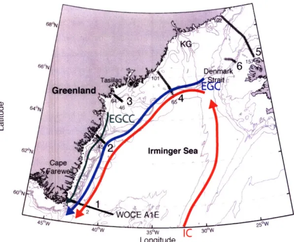
Figure 1.1. Regional map of part of the North Atlantic subpolar gyre showing a schematic of relevant upper layer currents, as well as bathymetric features and geographic names referred to in the thesis. Updating the circulation features in the boxed area is the focus of the remaining chapters in the thesis.
In addition to these oceanic processes, some mesoscale atmospheric processes (i.e. apart from the large-scale positive wind stress curl shown in Fig. 1.2. and the buoyancy-driven EGC) play an important role in the circulation of the Irminger Sea. These include barrier wind events, tip jets, and reverse tip jets, recently discussed by
may lead to deep convection in the Irminger Sea [Pickart et al., 2003], but the barrier winds can also affect the structure and strength of any potential coastal current along the southeast Greenland shelf, a concept discussed in detail throughout this thesis. Fig. 1.2 shows histograms of wind directions observed over one year (2004) at four latitudes along the southeast Greenland coast, illustrating the dominance of northeasterly winds to the north of Cape Farewell. These northeasterly winds are called barrier winds, and are
set up by the damming of air against the high Greenland continent, which results in a geostrophic flow of air towards the southwest. The predominant winds at Cape Farewell are southwesterly, reflecting the frequent passage of low-pressure systems that pass the southern tip of Greenland along the North Atlantic storm track. The high variability of winds at Cape Farewell strongly influences the behavior of the shelf circulation and the coherence of any coastal current flow, an idea discussed further in Chapters 2 and 3 below. Fig. 1.2 also illustrates the small spatial scales of the winds in the subpolar gyre.
Despite the potential for these low-salinity currents to move offshore and affect wintertime deep convection in the Labrador and Irminger Seas, and their links to the interior flow and the DWBC system discussed above, the near-shore region of Greenland has remained poorly studied. Recently, however, there has been a renewed interest in the East Greenland shelf region, sparked by the important role that freshwater fluxes seem to play in controlling regional ocean circulation and, ultimately, global climate variability [e.g. Bryan, 1986; Aagaard and Carmack, 1989; Curry et al., 2003].
The detailed mechanisms by which this freshwater is transported within the polar and subpolar seas remain unclear, as do the precise magnitudes of the freshwater flux. It is thought, though, that boundary currents such as the high-latitude buoyancy-driven Norwegian Coastal Current, or the Alaskan Coastal Current, play a significant role in regional freshwater budgets [Mork, 1981; Weingartner et al., 2005]. How these coastal currents interact with the basin scale circulation, however, is also uncertain. The
interaction of river plumes (typically thought of as smaller scale coastal currents) with the outer shelf ocean circulation has received more attention both observationally and
shelves, freshwater is input not only from rivers but from melting sea ice, meltwater runoff from the mainland, and precipitation, resulting in coastal currents that are much
larger scale than the individual river plumes [Williams, 2003; Weingartner et al., 1999;
Fong et al., 1997]. '650N5;~ 67MN 7( 6E 6( 64 z SE 56 54 52 5C 50 46 x 10-' -55 -50 -45 -40 -35 -30 -25 -20 -15 -10 Longitude (-W) Ca arewel 60ON (6_3 0N Kk il/ /a3~~~r ~ ~ e _cs
Figure 1.2. Annual average wind stress curl (N m-3) taken from Risien and Chelton [2007, available online at http://numbat.coas.oregonstate.edu/quikcow/]. Black circles indicate positions for the wind roses. (insets) Histograms of wind directions at four latitudes (60'N, 630N, 650N, 670N) over the southeast Greenland shelf for one year. Data come from twice-daily scatterometer winds observed by the QuikSCAT instrument [available online at http://ssmi.com/qscat/qscatbrowse. html]. Dashed arrows point in the
along-shelf direction for each latitude.
Before delving into previous research on the EGCC in particular, it is beneficial to give an overview of the upper layer circulation shown in Fig 1.1. More information can be found in the review by Hansen and Osterhus [2000], and a thorough discussion of the regional water masses is provided in Chapter 2.
In the region of southeast Greenland (boxed region in Fig. 1.1), the Arctic-origin, low-salinity East Greenland Current (EGC) flows southward next to the Atlantic-origin, high-salinity Irminger Current (IC) near the shelfbreak. The combined transport of the EGC, the IC, and the DWBC is one measure of the subpolar gyre strength, with previous estimates in the range of 27-36 Sv, where 1 Sverdrup = 106 m3 s"' [e.g. Clarke, 1984; Bacon, 1997; Pickart, et al. 2005]. North of Denmark Strait, the EGC transport has been
estimated at -27 Sv, partitioned into a wind-driven barotropic component of-19 Sv and an 8 Sv baroclinic throughflow [Woodgate et al., 1999]. The discrepancy between these
numbers reflects the complexity of the region, with its many re-circulations, as well as the lack of direct measurements of velocity, since most studies use conservation of mass along with measured transport estimates to estimate regional volume budgets. An
example of this complexity is given by Holliday et al. [2007], who showed evidence of a retroflecting part of the EGC as it passes Cape Farewell, which significantly alters the circulation picture for the EGC as it transitions into the West Greenland Current. This retroflection could also bring freshwater into the center of the subpolar gyre more efficiently, yet the behavior of the EGCC as it passes Cape Farewell is still an open question; one that is discussed in Chapters 5 and 6 below.
The study of Bacon et al. [2002, hereafter B02] focused attention back on the shelf, inshore of the EGC and IC. B02 described a low salinity (S- 32.5) wedge of water trapped against the coast, reminiscent of previously observed high-latitude coastal
currents. Using vessel-mounted acoustic Doppler current profiler data and two
hydrographic stations southeast of Cape Farewell obtained during the summer of 1997,
B02 determined that the jet, which they named the East Greenland Coastal Current
(EGCC), transported -0.8 Sv. They suggested that this was mainly a seasonal feature resulting from coastal runoff. In 2001 the same feature was sampled with higher
resolution hydrographic measurements and was reported to transport 2 Sv of water
[Pickart et al., 2005]. This volume flux was surprisingly large, on the same order of the
1-2 Sv carried by the EGC in the vicinity of Denmark Strait [Hansen and Osterhus, 2000]. Furthermore, using the data from the Pickart et al. [2005] study, the associated
freshwater transport of the EGCC (referenced to a mean salinity of S = 34.956) was 57 mSv, almost 50% of the annual mean freshwater export from the Arctic Ocean through Fram Strait [Aagaard and Carmack, 1989]. Although this was a synoptic estimate, 57 mSv equals about four times the mean Alaska Coastal Current freshwater transport of 400 km3 yr-1, which constitutes a significant fraction of the freshwater entering the Arctic Ocean through Bering Strait [Woodgate and Aagaard, 2005].
Measurements of the EGCC prior to 1997 and 2001 are sparse in both time and space; the oldest that exist date back to the joint Icelandic-Norwegian cruises of the
1950's and 1960's reported by Malmberg et al. [1967]. Using geostrophic velocities referenced with current meter data from shelf moorings, they found a transport of 1.6 Sv for the EGCC, although they referred to it as the East Greenland Current [Malmberg et
al., 1967]. A recent review of these and other historical CTD data confirmed the presence
of the EGCC along the southeast coast of Greenland [Wilkinson and Bacon, 2005;
Holliday et al., 2007]. When the surface 33.5 isohaline was used as a proxy, the EGCC
appeared to follow the 500 m isobath closely [Wilkinson and Bacon, 2005]. However, low surface salinities do not necessarily represent solely the EGCC feature, but could
suggest the presence of melting sea ice that occurs along the path of the EGC and IC. More recent drifter studies suggested a two-branched system on the East Greenland shelf with two distinct southward velocity cores: one located close to shore that is likely
indicative of the EGCC, and the other at the shelf break presumably associated with the EGC and IC [Reverdin et al., 2003; Jakobsen et al., 2003]. These observations were based on very few drifters, however, all of which entered the shelf from the interior Irminger Sea south of Denmark Strait, presumably by wind drift or mixing.
1.3
Data
Despite the growing interest and the available historical data, many basic questions regarding the EGCC remain unsatisfactorily answered. This motivated a field program, undertaken in the summer of 2004, to investigate the EGCC south of Denmark Strait. It resulted in the first high-resolution survey of the coastal current (station spacing on the
order of 5 km), carried out with the ice-strengthened vessel RRS James Clark Ross. The main goals of the cruise were to establish the existence of the coastal current, determine to what extent it was driven by coastal runoff (as surmised by B02), and obtain a basic description of its along-shelf evolution. The plan was to occupy a set of transects from
Cape Farewell to Denmark Strait, which would enable investigation of the current's origin, evolution, dynamics, and importance to the regional freshwater system.
The 2004 cruise took place in the fourth and final year of a broader project entitled "Is Labrador Sea Water formed in the Irminger Basin?". The observations
obtained in 2004 are the main source of data used in this thesis and are described in detail in Chapter 2. Additional sections occupied in the first three years of the project (2001
-2003) are also used in Chapters 2 and 3, and provide some temporal context for the more extensive observations of 2004. This project fit into the larger scale aims of the
Arctic-Subarctic Ocean Flux (ASOF) study, a multi-institutional, international collaboration focused on improving our understanding of the key fluxes between the Arctic and Atlantic Oceans. A basic understanding of these fluxes is needed in order to recognize any changes that may happen in a climate change scenario and to understand the forces that drive that variability.
Other sources of data are introduced as needed, and include satellite observations of sea ice concentration, wind records from the QuikSCAT scatterometer (both come from passive microwave instruments that penetrate through clouds), and a historical database of nutrient observations in the Denmark Strait region, among others.
Chapter 2
Hydrographic and velocity structure of
the East Greenland Coastal Current
2.1 Introduction
The primary aim of this chapter is to provide the first detailed description of the EGCC in terms of its salinity, density, and velocity structure, both in the across-shelf and along-shelf directions. Historical records of the EGCC, of which there are few, commonly refer to the coastal current as the EGC, obfuscating the distinction between the two flows that will become apparent in this and subsequent chapters. An emphasis, then, is placed on objectively defining the EGCC when it can be distinguished from the EGC to elucidate discussion of when the two currents may actually interact more fully. The description of the EGCC in this chapter then leads to a deeper understanding of the primary forces controlling the behavior of the EGCC and its variability. Parts of this chapter come from
Sutherland and Pickart [2007], with more discussion included here as well as a more
") V.
Longituae
Figure 2.1. Map of JR105 station locations (+ symbols) and the WOCE AlE transect (solid line) off Cape Farewell. The 200, 350, 500, 1000, 2000, and 3000 m isobaths from the GEBCO bathymetric database are shown in light grey [IOC et al., 2003]. Large numbers refer to JR105 sections, while the smaller numbers identify individual stations. KG denotes the location of the Kangerdlugssuaq Trough, while colored arrows denote the major upper layer currents schematically, similar to those in Fig. 1.1, but see Fig. 2.14 for an updated version of this circulation scheme.
2.2 Data and methods
The main source of data for this study comes from a July-August 2004 cruise on the ice-strengthened vessel RRS James Clark Ross (JR105) along the transects shown in Fig. 2.1. Six sections were occupied with a total of 170 hydrographic stations taken at high cross-stream resolution (3-5 km), with a Seabird 911+ conductivity/temperature/depth (CTD) system. Water to measure dissolved oxygen, salinity, and nutrient concentrations was obtained with a 12 x 10 liter bottle rosette. We used the salinity bottle samples to
calibrate the CTD conductivity sensor (accuracies are 0.002 for salinity and 0.001 C for the temperature sensor), while the nutrient water samples were analyzed on board for nitrate (NO3), phosphate (P0 4), and silicate (SiO4) concentrations with a Technicon AutoAnalyzer. A shipboard thermosalinograph continuously recorded surface temperature and salinity along the ship track. Direct velocity measurements were
obtained with a narrow-band, 150 KHz vessel-mounted acoustic Doppler current profiler (ADCP) that ran continuously during the cruise.
A key advantage of this data set is the high-resolution station spacing and the relative proximity to the coast of each inshore station (both on the order of 5 km). This represents the first oceanographic data set of its kind for the southeast Greenland inner shelf between Denmark Strait and Cape Farewell. We also have high-resolution data from transects taken in the summers of 2001-2003 by the R/V Oceanus (OC369 in 2001, OC380 in 2002, and OC395 in 2003) on the western end of the WOCE AlE repeat line off Cape Farewell (Fig. 2.1). These data were collected and processed identically to the JR105 data discussed here.
2.2.1 Hydrographic data processing
The CTD station data, consisting of salinity (S) and temperature (T), were pressure averaged to a resolution of 2 db. We then constructed vertical property sections by interpolating those data onto regular grids, with a resolution of 3 km in the horizontal and 10 m in the vertical, using a Laplacian-spline interpolation scheme. Potential density (oc) and potential temperature (0) fields, referenced to the sea surface, were constructed from the gridded sections at identical spacing.
Bottom depth profiles along the ship track were obtained from the ship's
multibeam sonar system, except during times of rough sea state when the CTD altimeter data were used to determine the water depth at the station sites. Most CTD stations attained a maximum depth of less than 5 m from the bottom. The bottom profile for the portion of each section from the inshore-most station to the Greenland coast was
interpolated from the General Bathymetric Chart of the Oceans (GEBCO) one-minute gridded bathymetric data set [IOC et al., 2003].
2.2.2 Velocity data processing
The calculation of geostrophic velocities requires density differences that are available from the gridded oa fields, but the main challenge is determining the reference velocity after integrating the vertical shear. This was done by using the concurrent direct velocity measurements taken by the shipboard ADCP, which introduced several
additional processing steps. First, in order to reference geostrophic velocities to a suitable ADCP velocity, the effect of the tides and other ageostrophic motions in the ADCP data must be minimized. The barotropic tidal signal was estimated and subtracted out of the velocity data as part of the shipboard processing using the Egbert et al. [1994] tidal
model (TPXO6.2). The model has shown good results in previous studies in this region [see Torres and Mauritzen, 2002; Pickart et al., 2005]. Errors associated with the de-tiding procedure come largely from inaccuracies in the bathymetric data available for the
Greenland shelf, so tidal velocities there may be biased by several cm/s [Torres and
Mauritzen, 2002]. The high velocity of the currents we are studying, 0(50 cm s'-), gives
us confidence that detiding errors will be insignificant; their contribution to error estimates for the transport values is discussed in Appendix A.
Second, although care was taken in trying to sample perpendicularly across the main jet features on the shelf and slope (whose mean path is expected to parallel the isobaths), maximum velocity vectors were sometimes oriented at an angle to the transect line. By rotating each velocity section into a streamwise coordinate system, a
methodology originally developed for Gulf Stream studies, any bias associated with how the current changes its orientation with respect to the bottom bathymetry is minimized
[Halkin and Rossby, 1985; Fratantoni et al., 2001]. Such a coordinate transformation was
applied to the JR105 ADCP data following the steps outlined by Fratantoni et al. [2001]. Care was taken to keep the observed jet features on the shelf (the EGCC) and over the slope (the EGC/IC system) separate in the analysis.
The de-tided and rotated ADCP velocities were interpolated onto the same regular grid as the hydrographic variables. Surface ADCP bins were excluded and the maximum depth of observations was 400 m off the shelf or 85% of the total bottom depth in water less than 400 m deep. Absolute geostrophic velocities in the alongstream direction, Uabs, were calculated by combining the geostrophic velocities, Ug, with the alongstream ADCP
velocities, Uadcp. The method we used matches the average velocity of Uadcp and Ug over
the depth range of available ADCP data at each horizontal grid point, such that
Uabs(X,Z) = Ug(x,z) + Uref (X) (2.1)
where the reference velocity, Uref, is defined to be
Urei(x) = f U d(x,z)dz - UfU(xz)dz (2.2)
which equals the difference between the mean ADCP velocity and geostrophic velocity over the depth range h. In all of the JR105 sections, Ure, 0, which implies that using
solely the baroclinic velocities would inaccurately estimate the speed of both the EGCC and EGC. Throughout the rest of the paper, we refer to the alongstream absolute
geostrophic velocity, Uabs, simply as velocity, and explicitly define other velocities as they are needed.
2.3 EGCC hydrographic and velocity structure
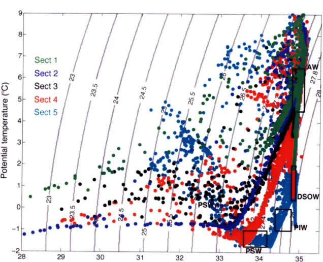
Several previous studies have documented the 9/S properties of waters near the East Greenland shelfbreak and their along-shelf evolution [e.g. Krauss, 1995; Rudels et al., 2002]. On the offshore side of the EGC/IC system is a water mass historically referred to as Irminger Sea Water [Clarke, 1984] with approximate 0/S properties of 4-50C andS-35. This is believed to be a product of mixing between the EGC and IC, influenced as well from heat loss due to intense atmospheric forcing during the winter months. In the interior of the basin lies Northeast Atlantic Water, a Gulf Stream remnant water with 0 > 70C and S > 35, that has undergone little modification since first entering the region
simplicity, we combine the two Atlantic-influenced water masses into a single, saline Atlantic Water (AW) type identified in Fig. 2.2 with 0 - 4.5-6.50C and S - 34.8-35.1.
The cold, low salinity waters near the shelfbreak and on the shelf originally derive from the Arctic and can be classified into three water masses: Polar Intermediate Water (PIW), Polar Surface Water (PSW), and warm Polar Surface Water (PSWw) [Rudels et
al., 2002]. PIW is the densest of these, defined as water with as > 27.70 and 0 < 00C that
comes from the colder parts of the Arctic Ocean thermocline. PSW is lighter with ce < 27.70, but can be very cold, with 0 < 00C. However, melting sea ice warms and freshens
this PSW, which also warms slightly on its way south due to air-sea interaction. This transformed water mass, PSWw, can exhibit a range of 9/S properties depending on the processes modifying it, although in general PSWw is lighter than PSW and warmer than 0 > 00C, as shown in Fig. 2.2.
2.3.1 Defining the EGCC
The main goal of this section is to provide an objective definition of the EGCC as a component of the Irminger Sea boundary current system. To accomplish this we utilize not only the 0/S properties and water masses described above, but we also present vertical
sections of the hydrographic properties and velocity from JR105. We emphasize this descriptive aspect of the study since older studies, based on sparser data, could not consistently distinguish between the EGCC and the EGC.
We start with the EGC, where numerous definitions have been used in the past based on hydrography: Pickart et al., [2005] used the 34.9 isohaline to distinguish the
EGC from the IC, while Nilsson et al., [2006] considered just the freshest part of the EGC using S < 34.5 as their EGC delimiter. Older studies also commonly looked at the freshest part of the EGC only (S - 34-34.9), if the current was distinguished from the IC at all [Clarke, 1984; Krauss, 1995]. In retrospect, some of these studies were probably sampling part of the EGCC and not recognizing its distinct nature from the EGC. Using these past studies as a guide, we use the 34.8 isohaline to mark the boundary between the
0 Q. E co it• C: Salinity
Figure 2.2. 9/S diagram for the entire JR105 data set indicating Irminger Sea and southeast Greenland shelf water mass definitions, which are Atlantic Water (AW), Polar Surface Water (PSW), Denmark Strait Overflow Water (DSOW), Polar Intermediate Water (PIW), and warm Polar Surface Water (PSWw). See text for discussion and specific water type property ranges.
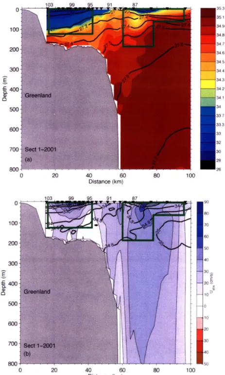
Objectively defining the EGCC as a distinct feature from the EGC is a separate issue, since their salinity ranges can overlap. Thus, to distinguish the EGCC from the EGC in this study we use a combination of velocity and salinity criteria. Specifically, we define the horizontal limits of the EGCC by where the velocity decreases to 15% of the maximum inner jet velocity. This defines the width, Wobs, of the observed current, while the depth, hobs, where the 34-isohaline intersects the bottom is taken as a vertical scale for the EGCC. For example, at Cape Farewell the EGCC is outlined by the inner green box
l o
in Fig. 2.3, which contains the 14 cm s' isotach that is 15% of the 95 cm s"' maximum velocity observed. Defined this way, the EGCC has a width scale, Wobs, of 30 km and a depth scale, hobs, of 75 m.
Similarly, the EGC is outlined by the outer green box that is drawn to satisfy the same velocity criteria used for the EGCC (in this case to capture the 9 cm sl " isotach since the max velocity - 60 cm s'), and the salinity criteria S < 34.8. The boxes are meant only as guides to show where the salinity and velocity criteria are used to delineate the EGC from the IC and the EGCC. Transports and freshwater fluxes, as well as the depth and width scales of the two currents, are computed using the gridded data that satisfy these specific velocity and salinity criteria.
Vertical sections of salinity and velocity for all the JR105 transects, displayed in Fig. 2.3-2.7, are the best indicators of the current; these two fields are shown in relation to each other to illustrate the basic structure of the EGCC. Temperature, although an important identifier of water masses, plays a relatively small role in controlling the density of the upper-layer boundary currents in the subpolar region.
Discussion of the possible reasons for the differences in the hydrographic and velocity structure along the path of the EGCC is deferred until section 2.4 of this chapter, as is an explanation of the variability seen in the EGCC at Cape Farewell during the summers of 2001-2003.
2.3.2 Section 1
-
Cape Farewell (60*N)
We start in the south at Cape Farewell to facilitate comparison with previous
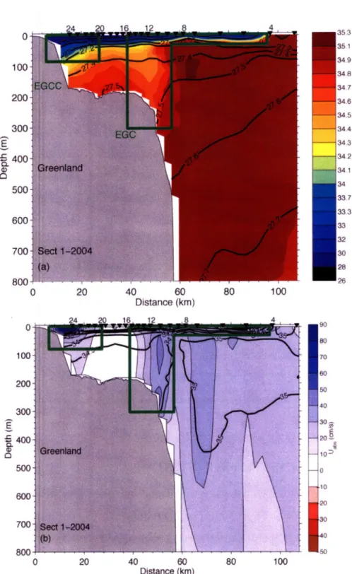
observations of the EGCC. Fig. 2.3a displays the salinity field and illustrates several important features. First, the strong front near stations 10-11 separating polar origin water and Atlantic-influenced high salinity water is the EGC/IC front, although the surface expression of the front is found 40 km farther offshore. The near vertical isohalines distinguish the AW, with S > 34.8 in the IC, from the EGC waters with S < 34.8. No PSW exists this far south, as it has been modified extensively along the path of the current becoming PSWw as shown in Fig. 2.2.
0 100 200 3001 400 500 600 700 800 0 100 200 300 500 600 700 800 9 8 7 6 5 4 3 [34,2 7 3 0 20 40 60 80 100 Distance (km) V0
so
r70 60 so50 40 30F 20 1o0 0 -20 .30 4t0 0 20 40 60 80 100 Distance (km)Figure 2.3. (a) Salinity field (color) from 2004 JR105 section 1 near Cape Farewell (60'N) with select isopycnals (kg m-') contoured in black. Boxes outline the boundaries defined in the text for the EGCC and the EGC. Black inverted triangles mark the numbered CTD stations. (b) Alongstream absolute velocity, Uabs (color, cm s'), for 2004 JR105 section 1 where Ua > 0 denotes equatorward flow. The isohalines (34, 34.5, 34.8, and 35) used in defining the currents are contoured in black.
,, 8O 7O 6O 5O 40 o .1o .20 -50
Inshore of station 20, a very fresh wedge of water, S < 32, lies over the shelf
roughly 20 km shoreward of the EGC/IC front. This is the front associated with the
EGCC. The 34-isohaline descends to a depth (hobs) of about 75 m at the coast, which is much shallower than observed in 2001 when hobs ~ 110 m (Pickart, et al. 2005), or in
1997 where observations showed no water with S> 34 at the innermost CTD station
(B02). Another feature seen only in 2004 is the low-salinity surface waters that extend out from the shelfbreak with an average depth of about 10 m. This is roughly the mixed
layer depth (computed where so - o,surfce > 0.125 kg m"3), which varies in the shelf region from 6-10 m, suggesting the important influence of wind and/or other mixing processes to the EGCC and EGC. This feature also implies that using surface
hydrographic or satellite data to infer the position of the EGCC can be misleading, since in this case the 34-isohaline outcrops almost 100 km from the coast, while the two currents are actually found much closer inshore. Mixed layer depth estimates in the region just offshore (east of station 4) of this fresh, surface cap are much deeper and average about 60 m.
The absolute geostrophic velocity section shown in Fig. 2.3b supports the salinity section in distinguishing the EGC from the EGCC. Associated with the low salinity wedge on the inner shelf, a distinct jet is observed with maximum velocities > 90 cm s-and significant alongstream flow throughout the water column. Note that we did not cross the entire current, so that extrapolation was necessary to obtain volume and freshwater transport values of the EGCC at this location (see below). A region of near-zero velocity separates the EGCC from the high velocity EGC core centered near the salinity front at station 11. Offshore of the EGC near station 7 is a deep-reaching velocity core that likely corresponds to the IC. In previous studies, the IC and EGC were reported as a merged system in velocity, though they were easily distinguished in 0/S space [Pickart et al., 2005]. In 2004, however, the two currents are distinct in their velocity signals as well.
2.3.3 Section 2 - near 63*N
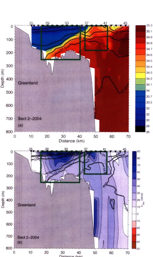
Section 2 is located approximately 350 km to the north on the narrowest part of the southeast Greenland shelf at 63*N (Fig. 2.1). Again, a wedge of fresh water dominates the salinity structure in Fig. 2.4a over the shelf, although it is much deeper at the coast
(hobs ~ 200 m) than the wedge seen at Cape Farewell. The water found here contains a
stronger core of modified PSW, with the freshest water shown in Fig. 2.2 much colder, 0 < 00C, than at section 1. The influence of warm, salty water is still present though, with
the eroded PSW core on a mixing line with AW. The EGC/IC front on this section is located near stations 37-38. Inshore of this front, mixed layer depths are deeper than observed at section 1, ranging from 10 -20 m, possibly in response to the stronger wind forcing that occurred during the occupation of this transect, but still shallower than offshore of station 40 where the average mixed layer depth is -50 m.
Associated with the sloping isohalines of the low salinity water on the shelf is a strong velocity signal (Fig. 2.4b) with maximum values near the surface exceeding 100 cm
s
"' and near-bottom values up to 30 cm s"'. Using the velocity and salinity criteria for defining the EGCC, we find that the majority of the flow found at this section isidentified as part of the coastal current, shown in Fig. 2.4b (inner green box).
Near the shelfbreak it is difficult to isolate the EGC (compared to the distinct EGC seen farther south in Fig. 2.3b). The confusion in nomenclature between the EGCC and EGC is most evident here, since many previous investigators would call the observed flow at section 2 the EGC, while we reserve that for the shelfbreak portion alone.
Bathymetry may play a part in this as the shelf is very narrow here (about 40 km wide versus > 100 km farther north), thus bringing the EGC and EGCC flows in close proximity. This may also explain why the velocities measured at section 2 are so large (the largest observed during the survey). We address the distinction between the EGCC and EGC later in this chapter, as well as the reason for the large velocities observed at this location.
100 200 300 E G400 500 600 700 800 20(10C E 40(
50(
60C 700 800 9 8 7 6 5 0 10 20 30 40 50 60 70 Distance (km) v0so
70 so 80 so 40 30-208~ 0 10 20 30 40 fso 0 10 20 30 40 50 60 70 Distance (km)Figure 2.4. Same as Fig. 2.3, except for 2004 JR105 section 2, which is near 630N.
3 2 7 3 ^^ w 8O 70 6O 5O 4O 10• 0 10 30 40 so
2.3.4 Section 3 - near 65°N
At this latitude the shelf contains an 800 m deep basin, and the JR105 section sampled only the inshore part of this basin (which extends very close to the coast), missing any shelfbreak flow. This implies that the current observed at section 3 is exclusively the EGCC. However the bathymetric influence of the basin extends out to the shelfbreak, so that a portion of the EGC could be diverted inshore around the basin. This notion is supported by studies showing southward-directed drifter tracks on both sides of the basin
[Reverdin et al., 2003; Jakobsen et al., 2003].
As in the sections to the south, we observed a fresh wedge of water at section 3, indicative of the EGCC. The freshest water shown in Fig. 2.5a is again the coldest, falling in the PSWw regime, although, unexpectedly, it is warmer than observed at section 2 as seen in Fig. 2.2. Another surprise is the presence of salty water, S > 34.8, found occupying the majority of the subsurface water column near station 46, far inshore of the shelfbreak. This is also suggestive of flow diverting from the shelfbreak around the basin and bringing with it AW influence from the EGC/IC system, a notion supported by the thermosalinograph data in Fig. 2.8.
The velocity data in Fig. 2.5b display a surface intensified jet with maximum velocities near 60 cm s-1. At this location the EGCC is over 300 m deep and 30 km wide, although the 34-isohaline intersects the bottom near 150 m, which is comparable to other sections. Another notable feature in Fig. 2.5b is the subsurface velocity maximum
observed on the western edge of the basin near station 48. This might represent a deep cyclonic circulation around the basin, although it is uncertain since the other side of the basin lies outside of our station data.
0 100 200 300 E •400 500 600 700 800 Distance (km) 0 100 200 300 400 500 600 700 800 90 so 70 60 40 o 10o 0 10 20 30 40 50 60 Distance (km)
Figure 2.5. Same as Fig. 2.3, except for 2004 JR105 section 3, which is near 650N.
353 351 34,9 34.8 347 34.6 345 344 343 342 34.1 34 33.7 33.3 33 32 30 28 26 26
2.3.5 Section 4 - near 66
0N
Section 4, which lies north of Tasiilaq where the shelf reaches its widest point, is the closest the JR105 data come to the area covered historically by Malmberg et al. [1967] and more recently by Nilsson et al. [2006]. Fig. 2.6a displays the observed salinity field that has a large wedge of fresh water with S < 34 occupying a good portion of the 100 km wide shelf down to a depth of 150 m. Some fresh water also resides in the vicinity of the
shelf break, yet the dominant features there are the two lenses of salty water, S > 34.8 (centered at stations 73 and 79 respectively), likely associated with AW eddies originating from the IC. Such features have been observed previously [Rudels et al., 2002; Pickart et al., 2005] and represent a source of AW influence reaching onto the shelf. If these features mix isopycnally, the salty influence will extend beneath the fresh wedge and modify the subsurface waters of the shelf. Eddy activity at this latitude has been observed in drifter studies as well [Krauss, 1995], suggesting that warm, salty intrusions onto the shelf are common in this region.
The 8/S characteristics of the water at section 4 (Fig. 2.2) indicate the presence of pure PSW, some modified PSWw, and a strong AW influence. Also note the densest water here is similar to Denmark Strait Overflow Water (DSOW, see Fig. 2.2), a dense water mass with as > 27.8, 0 > 00C and S- 34.8-34.9. This dense water signature comes
from two sources; one obviously is the DSOW itself, as we sampled deep enough to catch some of the DWBC along the Greenland slope. The other source is from the recently described East Greenland Spill Jet that forms from dense water spilling off the shelf, originally discovered at this same location [Pickart et al., 2005].
The freshest and coldest water is located on the inner shelf, shoreward of station 93, where the low salinity wedge attains its maximum depth. Coincident with this deepening is a surface-intensified jet (Fig. 2.6b). In this sub-wedge, salinities are < 32
and the maximum velocity is -60 cm s1'. This is the EGCC and it is separated spatially from the shelfbreak flow. The previous studies of Malmberg et al. [1967] and Nilsson et
al. [2006] sampled only sparsely near this location, and consequently resolved only the
0 20 40 60 80 100 Distance (km) 120 140 160 10 20 30
g
6O 7C 80 0 Figure 2.6. Same as 80 70 60 50 40 307 2o o 0 .10 20 40 20 40 60 80 100 120 140 160 Distance (km)Fig. 2.3, except for 2004 JR105 section 4, which is near 660N.
10
2C 30CS4C
50 60 6C 7C 8C l = , .L.1 ~ .50Both studies referred to the corresponding flow as the EGC, while in fact with tighter station spacing and closer proximity to the coast, we find that the EGCC exists even this far north. Note that the seaward edge of the fresh water wedge, defined by the outcropping of the 34-isohaline near station 83, is not associated with a strong jet (Fig.
2.6b). This is another example of the care one must take when considering only surface
data to describe the EGCC. In this section there is actually weak flow associated with most of the fresh wedge.
By contrast, the EGC is confined to a shallow depth near the shelfbreak, centered near station 69 in Fig. 2.6b, and adjacent to the salty lenses noted above in the salinity
field. The strongest flow observed near the shelfbreak actually resides just over the slope centered at a depth of 500 m near station 69; this flow is identified as the East Greenland Spill Jet previously described by Pickart et al. [2005] at this exact location. The
subsurface velocity maximum in Fig. 2.4b on the upper slope is likely a spill jet remnant as well. The IC is usually observed at this latitude; we assume its absence is due to the limited offshore extent of the transect and the presence of the strong spill jet feature.
2.3.6 Section 5 - north of Denmark Strait (68*N)
Section 5 was occupied north of Denmark Strait, extending from the Greenland coast to the Icelandic coast; however, the focus here is on the northwestern portion of the transect only. The dominant feature of the salinity field in Fig. 2.7a is the EGC front located near station 128. The isohalines descend about 200 m indicating the presence of the EGC in the middle of the basin upstream of Denmark Strait. The fact that the EGC is situated far offshore of the shelfbreak is not uncommon at this latitude; it has been observed detached from the shelfbreak previously and can re-attach downstream of the strait [Rudels et al., 2002; also see discussion in Chapter 4]. Water with potential density os > 27.8 kg m"3 is usually associated with DSOW. On the Greenland side of the EGC front, the water is lighter than this to about 300 m depth, indicating the presence of Arctic-origin surface waters. Farther south at section 4, this isopycnal is situated off the slope near the sill depth of Denmark Strait (- 600 m) in Fig. 2.6a. Unmodified PSW and PIW exist at
section 5, corroborated by the 9/S characteristics displayed in Fig. 2.2a. The water lying in the AW area actually comes from the Icelandic Irminger Current flowing to the north adjacent to the Icelandic coast (not shown in Fig. 2.7).
Interestingly, even though the upper layer is fresh between the Greenland coast and the EGC front, there is no pronounced wedge akin to the sections farther south. Rather, there is only a slight overall tilt to the 34-isohaline from the EGC front towards Greenland to station 108. Embedded within this tilt is a small region of enhanced thermal wind shear and a weak maximum in velocity centered near station 114 (Fig. 2.7b). We take the EGCC to be the flow contained within the inner green box in Fig. 2.7b, which has velocities up to 30 cm s-1 and reaches a depth of 200 m.
By contrast, the EGC signature is very strong at this section, with a surface intensified expression having velocities up to 60 cm s-1. Note the bowl-shaped structure of the deep isopycnals between stations 118 and 130. This corresponds to a recirculation over the deep basin with poleward flow on the western side of the outer green box. Whether or not this is a permanent feature is unknown, but it is clear that at the time of the survey not all of the observed EGC jet continued equatorward. Accordingly, we include the poleward part of the flow in defining the EGC and limit its depth extent to water with oe < 27.8 kg m"3, excluding any DSOW water.
9 8 7 6 4 3 ý 342 7 3 0 20 40 60 80 100 120 140 160 180 Distance (km) 0 100 200 300 E
4
00
500 600 700 800 f 9o 80 70 60 so 40 30, 20 10 0 20 -so 0 20 40 60 80 100 120 140 160 180 Distance (kmin)Same as Fig. 2.3a, except for 2004 JR105 section 5, which is Figure 2.7.
7t
II$
c
I
--S 6 i% si
t
t
so near 68°N.2.4 Sources of variability in the EGCC
As noted earlier, we observed a very fresh, S < 32.5, surface layer of water extending 100 km from the Greenland coast (Fig. 2.3a) in the JR105 CTD transect near Cape Farewell. This feature is present as well in the thermosalinograph data collected during the
occupation of the transect (Fig. 2.8, discussed below). However, the ship made additional crossings of the shelf and shelfbreak in the vicinity of Cape Farewell during the mooring work offshore, and the thermosalinograph data from six days before the CTD transect shows that the S < 32.5 water was confined closer to the coast inshore of the shelfbreak. One possible explanation for this, as well as for the alongstream variability in the volume transport estimates (presented below in Chapter 3), is forcing by the wind, in particular the along-shelf wind stress, alon,,g. Fortunately, we can investigate the role of time varying
alon,,g on the EGCC at Cape Farewell since data were obtained in the three previous
summers (2001-2003) during our field program, as well as in summer 1997 [B02]. Other possible mechanisms that can explain the observed variability include the influence of the irregular shelf bathymetry off southeast Greenland, as well as internal variability due to nonlinear processes and instabilities of the current itself. The
bathymetric process is discussed briefly in Section 2.5 and is the main topic of Chapter 5, while the effects of nonlinearities on the EGCC is investigated in Section 2.4.3.
2.4.1 Dynamical scales of the coastal current
Numerous theoretical and observational studies have shown that along-shelf winds can affect a buoyant coastal current through an "Ekman-straining" mechanism [e.g. Fong and
Geyer, 2001; Lentz and Largier, 2006]. Downwelling favorable winds steepen the front,
tending to deepen and narrow the current as well as induce a barotropic velocity and reduce stratification within the current. Upwelling favorable winds shoal the foot of the front and widen the current through a thin mixed layer that moves offshore at a velocity that scales with the Ekman velocity. Theoretical estimates exist for the depth of the foot
of the front, hp = (2Qf/g ')1/2, and the width of the current, W, = (g' hp,)l2/f+ Wb, where Q
Wb is distance from the foot of the front to the coast [Yankovsky and Chapman, 1997]. These estimates have been tested for smaller scale coastal currents, but never for a large-scale flow such as the EGCC.
35 34.8 345 34 33 32 31 30 Longitude
Figure 2.8. (a) Surface salinity field, S, from thermosalinograph data taken during JR105. The two lines near Cape Farewell are offset to allow visualization; one was taken during the CTD station work, while the other was taken during mooring deployments that preceded the CTD transects. (b) Surface temperature field, T ('C), from thermosalinograph data taken during JR105.
It is also useful to determine if a buoyant coastal current is "surface-trapped" or "slope-controlled". The former implies that the current is not influenced significantly by the bottom and may be more susceptible to the wind, while the latter suggests that bottom friction and bottom boundary layers play a large role in controlling the current. Previous studies have also attempted to separate the wind-driven and buoyancy-driven components
of a coastal current by defining a wind strength index, W, = u,wind/ ub,,oy [Whitney and Garvine, 2005]. W, compares the wind-driven and buoyancy-driven along-shelf velocity
scales. If
I
W, < 1, the flow is in a buoyancy-driven state, while for I W, > 1, strong windevents dominate the flow. These scales are defined and discussed below in Section 2.4.2 with application to the EGCC.
We now test these theoretical ideas with the observations of the EGCC along-shelf flow at Cape Farewell. To be complete, we first display the salinity and alongstream velocity sections at Cape Farewell from 2001-2003 in Figs. 2.9-2.11. They are presented identically to the JR105 sections above.
Table 2.1. The observed depths and widths of the
EGCC defined in the text, ho,b, and Wobs, along with
Ao,, / Aoff for each secton.
Section hobs (m) Wobs (km) Aon / Aof
1 75 30 0.18 2 190 24 0.6 3 150 27 0.1 4 110 30 0.02 5 110 20 N/A 1(2001) 100 28 0.14 1(2002) 140 24 0.11 1(2003) 65 21 0.09 1 (1997a) 110 24 N/A
0 100 200 300 400 500 600 700 800 C 100 200 300
j
40
500 600 700 800 53 5,1 49 48 47 46 4.45 44 4.3 [-3442 7 3 0 20 40 60 80 100 Distance (km) 80 70 60 50 40 30-20 10 0 .10 30 40 ,• 0 20 40 60 80 100 Distance (km)Figure 2.9. Same as Fig. 2.3, except taken in 2001 (OC369) near 600N at Cape Farewell.
^^

![Figure 1.2. Annual average wind stress curl (N m- 3 ) taken from Risien and Chelton [2007, available online at http://numbat.coas.oregonstate.edu/quikcow/]](https://thumb-eu.123doks.com/thumbv2/123doknet/14755572.582338/16.918.246.653.261.891/figure-annual-average-risien-chelton-available-oregonstate-quikcow.webp)