Dynamic scale modeling of bed configurations.

DYNAMIC SCALE MODELING OF BED CONFIGURATIONS

by

LAWRENCE ALLEN BOGUCHWAL B.A., Harvard College

(1972)

SUBMITTED OF THE

IN PARTIAL FULFILLMENT REQUIREMENTS FOR THE

DEGREE OF

DOCTOR OF PHILOSOPHY at the

MASSACHUSETTS INSTITUTE OF TECHNOLOGY

OCTOBER, 1977

Signature of Author

Department of Earth and Planetary Sciences, October 14, 1977 Certified by ... Thesis Supervisor Accepted by ...

Undmrd#

IES

DYNAMIC SCALE MODELING OF BED CONF.IGURATIONS by Lawrence Allen Boguchwal

Submitted to the Department of Earth and Planetary Sciences on October 14, 1977 in partial fulfillment of the requirements

for the Degree of Doctor of Philosophy.

ABSTRACT

A test was conducted proving that dynamic scale modeling of bed configurations is possible and that the following set of seven indepen-dent variables must fully characterize bed configurations: gravitational acceleration g, mean flow velocity U, mean flow depth d, fluid density p, fluid viscosity p, sediment density ps, and median sediment size D. For the test, conditions for two flume runs, one a hot-water model, the other a cold-water prototype, were adjusted according to a scale ratio of 1.66. Coincidence of cumulative frequency curves for the prototype and scaled-up model for each dependent variable, ripple height, ripple spacing and ripple migration time showed that the two runs were dynamically similar. Equations specifying dynamic similitude are lr = (P/P) 2/3 and (P /P)r

1, where 1r is the length scale and subscript r represents a ratio be-tween prototype and model.

Verification that the above set of seven variables fully charac-terizes bed configurations validates a three-dimensional diagram proposed by Southard (1971) based on a dimensional analysis of these variables in which mean flow depth, mean flow velocity, and median sediment size are correlated one-to-one with bed phase for constant water temperature and quartz-density sand. Existing flume data measured at different water temperatures were compared in this diagram by identifying the bed form hierarchy observed and by using the dynamic similitude equations to derive the dynamic equivalent for every flume run to one made at a standard temperature of 10'C. Boundaries separating bed phases were fully delineated in five velocity-size diagrams for 8.5 to 50 cm flow depth, eight depth-velocity diagrams for 0.13 to 1.60 mm sand size, and one depth-size diagram for 60 cm/sec flow velocity, by interpolation in three dimensions between orthogonal and parallel projections of the diagram.

Some of the most interesting relations among bed-phase stability fields were pinch-outs of fields, observed in the following projections: in velocity-size diagrams, the ripple field with increasing sediment size and bar, dune, and lower flat bed fields with decreasing sediment size; in depth-velocity diagrams for medium to coarse sediment sizes, the lower flat-bed field with increasing depth and the ripple and upper flat-bed fields with decreasing depth; in depth-size diagram, the bar, dune, and upper flat-bed fields with increasing depth, giving way to ripples or no movement at great depths.

- 3

-Based on the depth-velocity-size diagram, the effect of a change in temperature on the observed configuration can be determined. Given the initial conditions and the temperature chanae, the standard tempera-ture equivalent to each end state is located in the depth-velocity-size diagram and the bed phase and contour each plots on are identified. Con-tour values are then scaled to their equivalents at the observed tempera-tures.

A pilot study was carried out to determine the practicality of dynamic scale modeling using hot water with a flume and scale ratio larger than were used for the modeling test. Using hot-water modeling

for scale ratios up to about 2.5 on a very large flume, natural depths can be simulated. Using hot-water modeling on a small flume, a larger

flume can be simulated, representing many cost-effective savings and making existing flumes more flexible tools for research. While a pro-cedure for hot-water modeling with a covered, insulated flume was being developed, experiments were made in which certain of the relations

ob-served in the depth-velocity-size diagram were confirmed.

For sand sizes between about 0.1 mm and 0.3 mm, the sequence of bed states with increasing flow velocity is: ripples, continuous-crested

bars comparable to ripples in height but with significantly greater spacings comparable to dunes, discontinuous-crested bars with somewhat deeper troughs, continuous-crested dunes whose spacings and trough lengths steadily increase with velocity while heights increase but then decrease, and upper flat bed. With decreasing sand size the interval of velocity over which bars and dunes are stable steadily decreases and disappears at about 0.13 mm for 50 cm flow depth. Near the "point" of pinch-out distinction of bed forms is somewhat blurred as bed forms appear to possess attributes of adjacent stability fields. In addition to these results, data for bed-form height from this and other studies were summarized in qualitatively contoured depth-velocity and velocity-size diagrams.

These results confirm the extension of the bar stability field into fine sand sizes, the pinch-out of bar and dune stability fields with de-creasing sand size, the subdivision of the bar field according to bed-form hierarchy, and the subdivision of the dune field into dunes and flattened dunes. A plot of data onto the velocity-size plane agreed with boundaries of a velocity-size diagram (for 50 cm flow depth) constructed by three-dimensional interpolation of boundaries in the depth-velocity-size diaqram. Thus, placement of boundaries in the depth-velocity-depth-velocity-size diagram must be generally correct. Given the practicality of hot-water modeling and the consolidation of existing flume data, a velocity-size diagram for 2.5 m flow depth was constructed as a rough guide for the next generation of deep-water flume experiments.

To my parents,

-5-TABLE OF CONTENTS Page No. TITLE PAGE 1 ABSTRACT 2 .DEDICATION 4 TABLE OF CONTENTS 5 LIST OF SYMBOLS 8 LIST OF FIGURES 9 LIST OF TABLES 12 ACKNOWLEDGMENTS 13

PART I: SCALE MODELING OF BED CONFIGURATIONS 14

INTRODUCTION 14

Motivation for this study. 14

Overview of dissertation. 15

PRINCIPLES OF SCALE MODELING 16

Dynamic similitude. 16

The fundamental set of variables. 20 Determination of dynamic similitude for bed

configurations. 23

Laboratory implementation of scale modeling. 26

PART II: TEST OF DYNAMIC SCALE MODELING 29

CRITERIA FOR TEST 29

PROCEDURE 30

Apparatus and determination of independent

variables. 30

Measurement of dependent variables. 35

Page No. RESULTS AND DISCUSSION

PART III: SYNTHESIS OF EXISTING DATA INTRODUCTION

Correlation of fundamental variables with bed phases. Depth-velocity-size diagram. 49 49 Objectives. CONSTRUCTION OF DIAGRAM

Temperature normalization of data. Plotting the data.

Three-dimensional interpolation of boundaries.

DISCUSSION

Relations of bed-phase stability fields.

62 79 79

Temperature effects.

PART IV: PILOT STUDY OF HOT-WATER MODELING OBJECTIVES

PROCEDURE Flume.

Temperature control.

Measurement and error of depth and velocity. Selection of sand.

General operating procedure.

RESULTS

Presentation and description of data.

Contouring the depth-velocity-size diagram. DISCUSSION 91 93 93 97 100 101 102 105 105 121 126

-7-Page No.

PART V: SUMMARY OF CONCLUSIONS 132

BIBLIOGRAPHY 138

APPENDIX 143

LIST OF SYMBOLS AND THEIR DIMENSIONS

m Dimension of mass or number of fundamental dimensions

1 Dimension of length t Dimension of time

A Average, equilibrium height of bed forms (1); Area (1 )

b Width of flow (1)

D Median grain diameter (1)

d Mean flow depth (1)

r Froude number = U/(gd) 1/2(1)

g Gravitational acceleration (1/t 2

l r Length scale ratio, prototype to model (relative to one) n Number of independent variables in the fundamental set Q Flow discharge (1 3/t)

q Flow discharge per unit width (1 2/t) E Depth Reynolds number = Ud/v (1) S Regional slope (1)

T Temperature, *Celsius

tm Mean, equilibrium ripple migration time (t)

U Mean flow velocity (l/t)

A Mean, equilibrium spacing of bed forms (1) y Dynamic viscosity (m/lt) 2 V Kinematic viscosity (1 /t) p Fluid density (m/l 3) ps Sediment density (m/l 3 a Sediment sorting (1)

T Mean bed shear stress (m/lt 2 T₀ U Flow power (m/t3 )

-

9

-LIST OF FIGURES

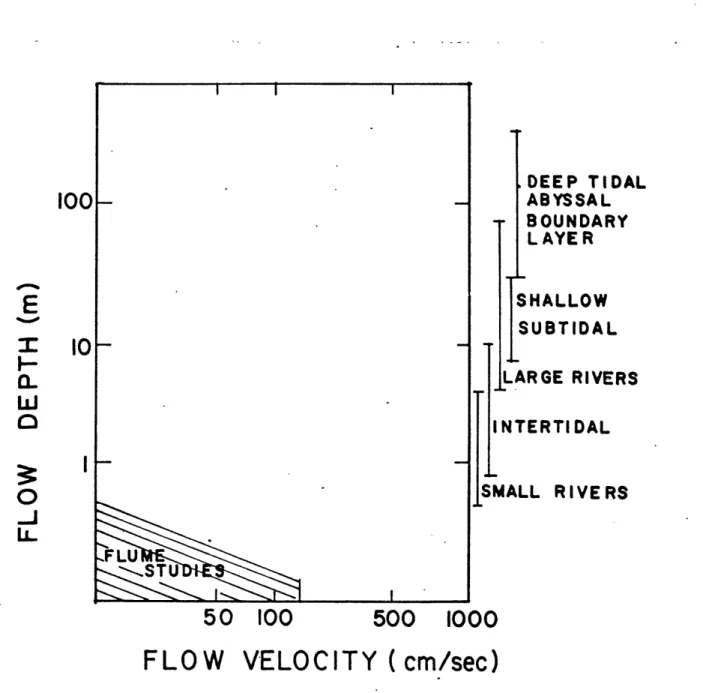
Page No. Fig. 1.1 Flow conditions for flume and field

studies. 17

Fig. 1.2 Scale ratios at different water

temperatures. 28

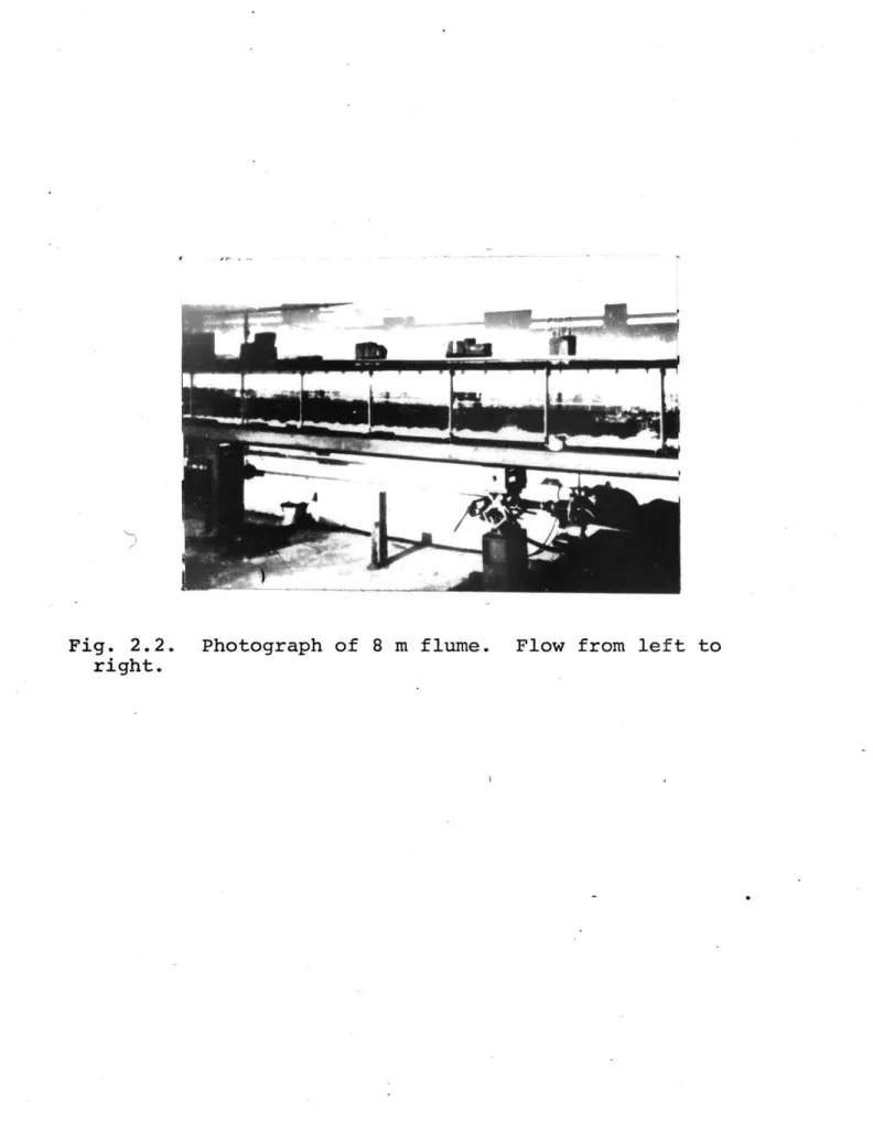
Fig. 2.1 Schematic diagram of 8 m flume. 32

Fig. 2.2 Photograph of 8 m flume. 33

Fig. 2.3 Photograph of typical ripple

configu-ration, model. 39

Fig. 2.4 Cumulative frequency curves for ripple

spacing. 42

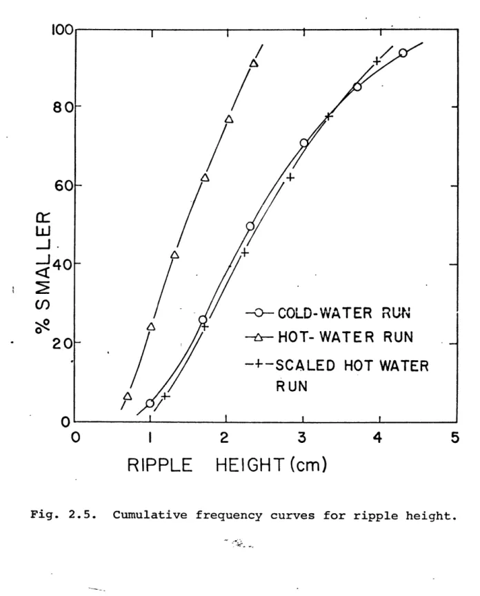
Fig..2.5 Cumulative frequency- curves for ripple

heights. 43

Fig. 2.6 Cumulative frequency curves for ripple

migration times. 44

Fig. 3.1 Velocity-size diagram for 8.5 cm flow

depth. 65

Fig. 3.2 Velocity-size diagram for 20 cm flow

depth. 66

Fig. 3.3 Velocity-size diagram for-30 cm flow

depth. - 67

Fig. 3.4 Velocity-size diagram for 40 cm flow

depth. 68

Fig. 3.5 Depth-velocity diagram for 0.13 mm

sand size. 69

Fig. 3.6 Depth-velocity diagram for 0.22 mm

sand size. 70

Fig. 3.7 Depth-velocity diagram for 0.31 mm

sand size. .71

Fig. 3.8 Depth-velocity diagram for 0.55 mm

sand size. 72

Fig. 3.9 Depth-velocity diagram for 0.62 mm

Page No. Fig. 3.10 Depth-velocity diagram for 1.07 mm

sand size.

Fig. 3.11 Depth-velocity diagram for 1.60 mm sand size.

Fig. 3.12 Depth-velocity diagram for 0.90 mm sand size.

Fig. 3.13 Depth-size diagram for 60 cm/sec flow velocity.

Fig. 3.14 Legend for Figs. 3.1-3.12 and 4.5. Fig. 4.1 Schematic diagram of 11.5 m flume. Fig. 4.2 Photograph of 11.5 m flume.

Fig. 4.3 Cumulative frequency curves of sands. Fig. 4.4 Velocity error bars for flume runs. Fig. 4.5 Plot of data onto velocity-size diagram

for 50 cm flow depth. -Fig. 4.6 Photograph of ripples. Fig. 4.7 Photograph of ripples. Fig. 4.8 Photograph of ripples. _. Fig. 4.9 Photograph of ripples. Fig. 4.10 Photograph of dunes. Fig. 4.11 Photograph of dunes. Fig. 4.12 Photograph of ripples. Fig. 4.13 Photograph of ripples. run IV-27. run IV-26. run IV-25. run IV-24. run IV-23. run IV-22. Linguoid Bars plus Bars plus Bars plus Bars plus Bars plus

run IV-8. Dunes plus

run IV-7. Dunes plus

4.14 Photograph of run IV-13. Dunes.

74 75 76 77 78 94 95 103 109 110 115 115 116 116 117 117 -118 118 119 Fig.

- 11

-Fig. 4.15 Photograph of run IV-15. Dunes. Fig. 4.16 Photograph of run IV-17. Flattened

dunes.

Fig. 4.17 Photograph of run IV-19. Flattened dunes.

Fig. 4.18 Velocity-size diagram (50 cm flow depth) qualitatively contoured for bed-form height.

Fig. 4.19 Depth-velocity diagram (0.30 mm sand size) qualitatively contoured for bed-form height.

Fig. 4.20 Velocity-size diagram for 2.5 m flow depth.

Fig. A.l _{Plot by source of data for Fig. 3.1.} Fig. A.2 _{Plot by source of data for Fig. 3.2.} Fig. A.3 _{Plot by source of data for Fig. 3.3.} Fig. A.4 _{Plot by source of data for Fig. 3.4.}

Page No. 119 120 120 124 125 131 144 145 146 147

LIST OF TABLES

Page No. Table 2.1 Experimental conditions for flume runs

of the modeling test. 41

Table 2.2 Mean and standard deviation of fre-quency distributions of experimental

characteristics. 46

Table 3.1 Sources used for diagram and the range

of normalized sediment sizes for each. 57

Table 3.2 Interval of control variable for each

projection. 61

Table 4.1 Summary of observations from pilot

study. 107

- 13

ACKNOWLEDGMENTS

It has been my privilege to work with Professor John B. Southard, without whose perceptive criticism and guidance in the scientific method this work would not have been possible. I wish to thank Professors Jon C. Boothroyd, Ole S. Madsen, David C. Roy, and Raymond Siever for their helpful comments on the final draft. I also wish to thank Professor Raymond Siever for the use of the 8 m flume at Harvard University.

For their cooperation and competence, I wish to acknowl-edge Sondra Hirsch, who typed this manuscript, Lohit Konwar, who drafted the figures, and Leroy Lindquist, who developed and mounted the photographs.

Those who offered a kind hand or bent ear when most needed are not forgotten. Among their number were fellow graduate students W. Russell Costello, William Corea, and Lohit Konwar, and my undergraduate assistants at various times.

Finally, to the person who shared my aspirations and frustrations, my wife Freda, I express my deepest apprecia-tion for her concern and promethean patience.

PART I: SCALE MODELING OF BED CONFIGURATIONS

INTRODUCTION

Motivation for this study.

To better understand sediment transport one must rely heavily on empirical studies. Laboratory simulations of sediment transport are valuable because conditions can be controlled, thus permitting constancy of conditions, isola-tion of particular variables, and ease of observaisola-tion--all largely unattainable in field studies of variable environ-ments. Models have been constructed on the scale of: a whole environment (for example, the fluvial simulations of Friedkin, 1945; Schumm and Kahn, 1972), bed forms (such as the flume studies by Guy et al., 1966), sand grains (such as studie's of forces on a grain by Chepil, 1961; Coleman, 1967). This study focuses on sediment transport on the scale of bed forms.

The usefulness of a model is limited by the extent to which it simulates its natural prototype. Observations of bed configurations in the field (for example, Boothroyd and Hubbard, 1975; Jackson, 1975) indicate that bed forms in natural environments are much larger, by factors of ten or more, than bed forms produced in laboratory settings. This disparity can be attributed to flow depth and width, the primary differences between conditions in the field and the flume. Nonerodible flume walls tend to restrict formation

- 15

-of large, broad bed forms and impose unnatural shear forces on the -configuration, apparent in relatively narrow channels with width-to-depth ratios less than about 5:1 (Williams,

1970). Furthermore, even with acceptable width-to-depth ra-tios, the flow depth in flume experiments is much less than depths observed in natural environments of greatest sedi-mentological interest (see Fig. 1.1). Although some studies

(for example, Yalin, 1977) suggest a linear correlation be-tween bed-form size and mean flow depth, there is no clear evidence that the effect of a depth change is a scale change from one configuration to another geometrically similar, as implied by these correlations. Nor is there evidence that these correlations can be applied across the gap between those depths in flumes and field environments, even if they are valid over the particular range of depths for which they were documented. Therefore, bed geometries and dynamics in flumes cannot be simply extrapolated to geometries and

dynamics occurring in deeper natural'settings; consequently, such simulations are only approximate.

Overview of dissertation.

To combine the strengths of the two approaches, the

natural scale of field studies with the control of laboratory simulations, one would either have to build a very large model or devise a true, nondistorting method of scale modeling (or both).

tested in Part II of this work. In addition to successfully demonstrating dynamic scale modeling for bed configurations, results of the test verify that the variables upon which the model is based fully characterize bed configurations. Ac-cordingly, in Part III a plot is constructed in which these va-riables are correlated with bed phases, making use of the previously developed scaling relationships so that data

measured at different temperatures can be compared. In Part IV a pilot study is discussed, which was carried out to

develop procedures for modeling at scale ratios larger than those in the test and to experimentally confirm interpreta-tions of the above plot. The chief conclusions of this study are summarized and evaluated together in Part V.

PRINCIPLES OF SCALE MODELING

Dynamic similitude.

When all significant corresponding forces--and therefore all dependent effects of these forces--in two systems scale consistently according to a specific relationship, the two systems are said to be dynamically similar. Thus, the non-distorting simulation proposed in the Introduction is a model that is dynamically similar to its prototype.

An equivalent way of expressing dynamic similitude be-tween two systems is that corresponding ratios of forces acting within each system are equal, where scale factors cancel out in each ratio. If an important force is left out

- 17

50 100

500

1000

FLOW

_{VELOCITY (cm/sec)}

Fig. 1.1. _{Approximate flow conditions for flume studies,} bottom left. At right, approximate depth ranges for

natural flows (after Middleton and Southard, 1977, p. 7.38). DEEP TIDAL ABYSSAL BOUNDARY LAYER #I 0

0j

in the modeling procedure, effects related to that force do not scale appropriately in the model.

One way of assuring that all important forces are con-sidered for a dynamic scale model is to work from the gov-erning equations of a system. If two systems are dynamically similar to one another, their dimensionless governing equa-tions will be identical since the scale ratios cancel out. For example, the governing equations that completely specify a one-component flow system are the Navier-Stokes equations. Dynamic scale modeling of one-component flow systems is

achieved by the numerical equality between two systems of the following set of dimensionless parameters: a Mach number, a Reynolds number, and a Froude number (each is essentially a force ratio). For incompressible fluids like water, dynamic similitude is specified by Eq (1.1), derived by equating corresponding Reynolds and Froude numbers of two systems:

-12/3

Few studies of free-surface systems based on Eq (1.1) have been made because of the demanding restrictions imposed

on the model. Many studies have been made of dynamically similar systems possessing no free surface because there are less stringent restrictions on the model components as only Reynolds number similarity is required. Froude number simi-larity is an example of approximate, nondynamic modeling used for simulations of large-scale free-surface flows where vis-cous effects, characterized by the Reynolds number, are

- 19

relatively small. In Froude models there is large-scale geometric similarity, but distortions of the forces require such adjustments as railroad spikes on the bed of a fluvial model in order to simulate certain characteristics (in this case, roughness) of the prototype. In fact, the "art" of -modeling has been to minimize distortions and judiciously interpret results from nondynamic models like these Froude models.

For this study complete similarity of forces.is desired, not just superficial geometric similarity or similarity by

artificially induced adjustments in the model. Also, unlike Reynolds similarity models, prototype systems of sediment

transport have a free surface; unlike those one-component

systems with a free surface to.which Eq (1.1) applies, sediment-transporting systems involve two components, fluid and sedi-ment. Consequently, additional modeling criteria are required.

Buckingham (1914) proved that the minimum number of di-mensionless force ratios necessary to specify a system is n-m; m is the number of fundamental dimensions used and n is the number of independent, fundamental variables that fully char-acterize the conditions of a system, from which the force ratios are derived. In most physical problems, m equals

three: mass, length, and time. If a variable is overlooked, then some dynamic aspect in the model is left unspecified. On the other hand, an extraneous variable unnecessarily and redundantly overspecifies forces acting in the system. Thus, the set of n fundamental variables and the set of n-3 derived

force ratios must be both necessary and sufficient in speci-fying the system studied.

Buckingham (1914) showed further that, in terms of uniquely and completely specifying a system, a set of n-3 force ratios is equivalent to any set of n-3 dimensionless parameters derived from a dimensional analysis of the same

fundamental set of n independent variables. This is because a set of n-3 parameters could explicitly represent any one of the many sets of force ratios, each of these latter sets being a particular group of force pairings. In addition, there are an infinite number of sets of n-3 dimensionless

parameters that could implicitly represent any of those sets of force ratios, since each parameter could theoretically be multiplied by any other dimensionless parameter to recover a particular force ratio (permitted as long as parameters are

not eliminated, leaving some aspect of the system unspecified). Thus, for dynamic similitude, the numerical values of

cor-responding dimensionless parameters between model and proto-type must be identical, just as numerical values of correspond-ing force ratios must be identical. A set of dimensionless parameters characterizing bed configurations is presented

after the following discussion in which the fundamental variables are identified.

The fundamental set of variables.

The many sets of variables used to characterize sediment transport on the scale of bed configurations can be roughly

- 21

-separated into four groups, originating or typically used by: Simons and Richardson (1963), Vanoni (1974), Southard (1971), and Maddock (1970). Common to all four groups is specifica-tion of the gravitaspecifica-tional acceleraspecifica-tion g acting on the system and the fluid by its density p and dynamic viscosity y.

Authors using slope as a variable, typical of the fourth group, do so generally because they study sediment transport on a larger scale, where regional slope is significant; this group will therefore not be considered further in this dis-cussion. _{(At least on the smaller scale of bed} configura-tions, slope is observed to be a dependent variable.) The sediment and flow are specified by the remaining three groups in various ways outlined below.

Sediment is specified by its density p₅ and by either

the mean or median grain diameter D. Since the median grain diameter is easier to measure than mean grain diameter, it will be used in this study. Vanoni (1974) and others also use a sediment sorting or standard deviation factor a. How-ever, since sorting has an effect essentially secondary to median grain diameter, effects of only median grain diameter will be focused on in this study. Hence, only relatively well-sorted sands are considered in this study.

The three groups differ most widely on the manner in which the flow is specified: the Simons group by flow power T ₀₀U and mean bed shear stress T , Vanoni by mean bed shear

stress T and mean flow depth d, and Southard by mean flow

mo-tion it is evident that two variables are required to specify the flow, equivalent to a depth and a velocity. Because mean bed shear stress is proportional to the velocity gradient, it can be used to characterize either velocity or depth. Simi-larly, flow discharge Q and flow discharge per unit width q are proportional to the product of velocity and depth, so that they too could characterize either velocity or depth. Therefore, one different variable from each of the two fol-lowing groups would characterize the flow: U, T0 ,TOU, Q, q

and d, T , T0U, Q, q.

Brooks (1958) showed that mean bed shear stress can be double-valued, where certain values specify two configurations rather than one. Although this does not invalidate sets using bed shear stress as a variable for scaling purposes, it does mean that such a set could possibly characterize the wrong configuration during a scaling procedure. If the same set of fundamental variables used for scaling are to be later cor-related with different bed configurations (see Part III), then variables of that set should be single-valued for explicit one-to-one correlation. Mean bed shear stress and flow power, therefore, are not used here as fundamental variables.

Furthermore, because a bed configuration could be thought of as forming in a sheet flow of infinitely wide extent, width is not considered a fundamental variable. Therefore, flow dis-charge per unit width is preferable to flow disdis-charge as fun-damental variables are selected. That leaves two of the three following variables for specifying the flow: d, U, q.

- 23

-From the above considerations, the following set of n = 7 fundamental variables is seen to characterize bed configura-tions: gravitational acceleration of the surrounding force field, density and dynamic viscosity of the fluid, density and median grain diameter of the sediment, and mean flow depth and mean flow velocity of the flow. This set charac-terizes the entire range of variability of bed configurations since the entire range of variability of the force field, the fluid, the sediment, and the flow are fully specified. One might be prompted to eliminate some variable from the set because its effect over some range of its variability is small. However, the full set of seven variables is the fun-damental set over all conditions since the concept of dynamic similitude is not restricted to a single narrow range of

variation.

That these seven variables comprise the fundamental set is both corr'oborated by dimensionless plots of these vari-ables versus bed phase (see Part III), which lack the scatter and overlap of points indicating omission of a variable and parallelism of points to an axis indicating an extraneous variable, and verified by the modeling test reported in Part

II.

Determination of dynamic similitude for bed configurations.

For n = 7, four dimensionless parameters are necessary

and sufficient to characterize bed configurations. One set that explicitly represents dimensionless force ratios is:

the Froude number U/(gd)1/ 2 , the ratio of gravity forces to

total inertial forces; a depth Reynolds number Ud/v, the ratio of viscous forces to inertial forces; p /p, the rela-tive density of the components; and d/D, an index of system geometry. These parameters are cast in a dimensional analysis based on quotients of U, d, and p.

Dynamic similitude for bed configurations between a prototype and model is expressed by the following set of

equivalencies between corresponding dimensionless parameters:

U= (1.2) (gd)l/2I Vr D r = (1.5) ( r

After realizing that mean-flow-depth ratio and median-grain-diameter ratio are equivalent dimensionally to any length scale, an arithmetic manipulation of the above equa-tions leads to the equaequa-tions governing dynamic similitude for bed configurations: (v2 1/3 1 = (1.6) r r = 1 (1.7)

(Ps

- 25

-For a prototype of quartz sand and water, there are two degrees of freedom for model construction. Selection of any two of the following quantities fixes the scale value of all other independent variables in a dynamically similar model: gravitational acceleration scale, a length scale, a fluid, or a sediment.

For practical purposes, the gravitational acceleration scale will equal one for almostall laboratory models. The determining equations then reduce to:

= V2/3 (1.8)

= 1 (1.9)

S r

In Eqs (1.8) and (1.9) there is only one degree of freedom, where selection of only one of the following fixes the value of all other variables in a dynamically similar model: a length scale, a fluid, or a sediment.

That one of the above equations is identical to Eq (1.1) for one-component flow systems comes as no surprise: although the complete equations of motion for one-component and two-component flows must be dissimilar, they are both based on a set of variables specifying the flow. According to a theory of similarity, equivalencies of force ratios as expressed in Eqs (1.8) and (1.9) are a necessary condition for dynamic scale modeling. However, in the absence of governing equa-tions for two-component systems, only a comprehensive test as reported in Part II of this study can verify whether these

equations are sufficient for dynamic scale modeling of bed configurations.

Laboratory implementation of scale modeling.

The limiting factor in Eqs (1.8) and (1.9) has to be selection of the model fluid. Even modest scale ratios re-quire kinematic viscosities for the modeling fluid that are substantially lower than water. Of the few fluids that do allow even a modest scale ratio, up to about 4, all are either

flammable, toxic, volatile, prohibitively expensive, or un-available. Those compressed or cooled gases that appeared to have potential as modeling fluids usually share one or more

of these shortcomings and, more importantly, would not have a free surface, which the natural prototypes have. Required pressures up to about 70 atmospheres or temperatures down to

-15*C would also have to be dealt with.

Large scale ratios (greater than 15 to 20) are not feasible, primarily because proper modeling fluids do not exist; however, if one did exist, there would probably still be the presence of nonsimilar cohesive effects in the very fine sediment of the model. For these reasons, dynamic scale modeling of sediment transport has been largely ignored by engineers and geologists. However, if one focuses on sediment transport at the scale of bed configurations, even scale ra-tios as modest as 2.5 would prove worthwhile since the range of flow depths of such a model--up to 2.5 m--would definitely overlap that range of depths of greatest sedimentological

- 27

-interest (see Fig. 1.1).

A fluid that is safe, inexpensive, readily obtainable,

and properly wets its model sediment is water. At a tem-perature of 800C the scale ratio relative to a standard

temperature of 10*C (selection discussed in Part III) is about 2.33. For scale ratios for lesser temperatures in the model see Fig. 1.2; for scale ratios relative to different prototype temperatures divide the old scale ratio for

10 m

by the scale ratio for (maximum scale ratio about 2.75). new

Because the quotient (p /p) for water changes by only 3% with a temperature change from 0*C to 800C, quartz sand or

2-6

-2-2

[-8-10

10

30

50

70

90

oc

Fig. 1.2. Scale ratios at different water temperatures, relative to v = 1.31 cm2/sec, at 10C. (After Handbook of Chemistry and Physics, 1976.)

- 29

-PART II: TEST OF DYNAMIC SCALE MODELING

CRITERIA FOR TEST

A test was conducted in which dependent measures for two flume runs, a cold-water prototype and a hot-water model,

were compared to verify that Eqs (1.8) and (1.9) determine the conditions for dynamic scale modeling of bed configura-tions. The success of this test depended upon three factors:

1) the completeness of the set of fundamental variables (dis-cussed in Part I), 2) the adequacy of the test criteria,

3) the quality of the measurements. Yalin (1965) actually

made a test of dynamic scale modeling, but his results were limited to a suggestive photograph of two geometrically simi-lar bed configurations.

Since 'a fundamental set of variables implicitly speci-fies the forces acting in the system, the geometry and kine-matics of that system are also specified. If forces cannot

be measured directly, measures of both the geometry and kine-matics of each system should be compared. In this test the

geometry for each run was characterized by individual cumu-lative frequency curves for height and spacing of the observed bed forms, which were ripples. Ripple spacing was defined by the distance between brinkpoints of successive ripples, and ripple height was defined by the vertical distance between the brinkpoint and the lowest point of the trough immediately

downstream. Kinematics for each run was characterized by a cumulative frequency curve of ripple migration times (time

rates are motion-related and so are kinematic), defined by the elapsed time between passage of successive ripple crests past a reference section.

The dynamical aspects of each variable are most apparent when each is considered dimensionlessly as quotients involv-ing mass, gravitational and viscous forces: X ( l/3

A(g - ₁ t 2-). Corresponding curves for each variable should coincide if the two flume runs are dynamically similar. However, results are plotted dimensionally with one curve of each pair scaled to overlap the other, in order to illustrate the difference in results between scaled and unscaled data.

PROCEDURE

Apparatus and determination of independent variables.

B'oth runs were made in the same.tilting, closed-circuit flume, with 15.6 cm maximum width and 8 m length, which re-circulated both sediment and water (see Figs. 2.1 and 2.2). The channel itself was constructed of Plexiglas. The flow was pumped by a centrifugal pump, powered by a 1 1/2 hp motor, through a single 2" I.D. copper return pipe back to the head-box. Ambient inlet turbulence was damped by a baffle at the juncture of the headbox and channel and by straws placed just downstream. Surface waves at the inlet were damped by a

board resting on the water surface, placed downstream of the straws. Discharge was controlled by a gate valve mounted in the return pipe and was measured by a precalibrated orifice

- 31

-meter (dia-meter = 1.6") upstream of the gate valve. Discharge

readings were made from a U-tube manometer filled with s-tetrabromoethane for the low-discharge model run and mercury for the higher-discharge prototype run and connected to pres-sure taps off the orifice meter.

The nature of the experiment required that conditions be set and monitored with a precision unusual in flume experi-ments. Mean flow depth was defined as the time-averaged depth at the wall of a reference section, denoted by a vertical line on the flume wall. A 16-mm motion picture camera connected to a timing device photographed the flume wall at constant time intervals. Flow depth was measured from the movie film frame

by frame. Measurements of nearly 1500 frames from a trial

run showed statistically that measurement of 200 consecutive frames was sufficient to determine the mean flow depth to within 1 mm accuracy. Since the values of depth and velocity were specified for the model by measurements of depth and

discharge in the prototype (velocity was calculated from measurements of discharge, depth, and channel width), flow

depth in the model had to be first determined and then adjusted

by adding or subtracting water from the channel. Flow

dis-charge was also adjusted accordingly, in order to set the mean flow velocity for the model run; this procedure yielded a velocity accurate to within about 0.2 cm/sec.

During a run, flow depth was monitored constantly using a ruler taped to the flume wall. From these readings an

re-- 32

-I PUMP 58AFFLE & STRAWS 2 ADJUSTABLE SUPPORT6 WAVE DAMPER

30RIFICE METER 7 FLUME COVER 4 CONTROL VALVE

- 33

-Fig. 2.2. Photograph of 8 m flume. Flow from left to right.

placed at that approximate rate by means of a

valve-controlled, slowly dripping spout. The channel was covered to minimize water loss from evaporation.

Temperature for both runs also had to be carefully con-trolled and monitored. For the cold-water prototype, water was drawn from the tailbox, circulated through a cold-water

reservoir cooled by a thermostat-equipped refrigeration coil, and returned to the tailbox at a point lower than from where it was drawn. Temperature for the hot-water model was con-trolled by a thermostat-equipped L-shaped immersion heater placed in the channel well downstream of the reference

sec-tion. Channel covers used during both runs minimized tem-perature variations, which were about ±10C, as monitored by

a thermometer in the channel.

For the purposes of this test, data mheasured at the

sidewall were just as valid as data measured down the center-line of the channel, provided that the manner of measurement was the same in both runs. Thus, the narrowness of the flume

did not affect the outcome of the test. However, because measurements of depth and also of the dependent variable were made from photographs of the sidewall, it was important that wall effects scaled from one run to the other. This was done

by scaling the width, using the full channel width in the

prototype and a false wall in the model. The false wall was constructed of smooth-surfaced bricks, 25 cm high and exactly wide enough (6.2 cm) to fill the unused portion of the channel.

- 35

-from one run to the other, ambient inlet turbulence and in-let shear stress did not scale. Therefore, the reference section was positioned for both runs so that crossing ripples were fully developed, based on observations at equilibrium;

it was not positioned in the model according to a scaled -length downstream from the inlet because entrance effects

were unscaled.

Very well sorted sands were used, each having been sieved into 1/4-$ fractions: 0.23±.02 mm for the model and 0.38±.03 mm for the prototype. Although sorting was not a

variable, the very small standard deviation of each size did coincidentally scale.

Measurement of dependent variables.

Two methods for recording measurements of dependent variables were tried. The first amounted to a streamwise profile of the bed made at intervals of about three hours.

(Three hours assured independence of the successive profiles, as determined by visual observation.) The second was

time-lapse cinematography of about a one-meter reach. The second method was chosen over the first for the following reasons.

Migration time turned out to be the variable most sensi-tive to changes in the independent conditions, so it could be considered the most critical criterion of the test. Cumula-tive frequency curves of migration time did not match when using the first method, probably because the interdependence of adjacent ripple-migration rates statistically b-iased the

data. For the second method, migration times were recorded from individual ripples over a period of time sufficient to minimize interdependence of successive bed forms. Also, measurements at intervals of a few minutes instead of a few hours was far more likely to capture those transient varia-tions, such as the occurrence of short-lived, fast-moving ripples, that were an integral part of the statistical char-acterization of each run. Thus, a sequence of 100 ripples on film provided a more varied and therefore a more repre-sentative sample than a sample of ten profiles of ten ripples apiece.

Time-lapse cinematography provided a permanent record from which many dependent variables could be determined. The time interval was adjusted to capture a particular ripple about six times in the field of view. This adjustment was an economical use of film and a time-telescoping feature. The field of view spanned about three to four ripples. Both the time interval and field of view were scaled from proto-type to model to avoid any implicit bias in the data. A clock and a horizontal/vertical scale were kept in the field of view for references.

The easiest way to read the film was to mount it on a

35 mm downward-projecting microfilm reader. Thousands of frames were tediously scrutinized in dark corners of the

library. In the future, if the same film were to be analyzed for more than one purpose, digitizing would be highly recom-mended.

- 37

-According to the definition for ripple migration rate, the number of constant time intervals between frames was counted between successive crests crossing the reference section. Since the instant of crossing was generally not recorded on film, that time was interpolated by assuming a constant migration rate between two successive frames, one taken before and one after crossing the reference section. The crest position was recorded for each frame by laying a calibrated grid on the film projection, lining up reference marks on the grid with the reference section, and making a reading. About 100 ripples for each run were so measured.

Measurements of ripple spacing and ripple height made more efficient use of the film than measurements of migration times. Measurements were made every five frames, recording the position of every crest/trough pair in the field of view on a sheet of graph paper lying on the projection, and

taking measurements later. Ripples generally maintained their identity over this interval, but their form changed sufficiently that alternate configurations (every ten frames) were independent of one another. About 200 ripples were

measured for geometry for each run.

General operating procedure.

Once the initial conditions of a run were set, a period of about four days elapsed before filming commenced. During that time, the bed came to a dynamic equilibrium, achieved when a characterization of the bed configuration was the same

in successive observations. Depth was measured from the film and experimental conditions adjusted accordingly. After

another period of about four days, during which the bed was again observed to come to equilibrium, the final time-lapse film was shot. A typical configuration is shown in Fig. 2.3. - -A length scale of 1.66 between the two runs was based

on the limitations of temperature control in the cold-water prototype. Experimental conditions for model and prototype are described in Table 2.-; note that time and velocity di-mensions scale as the square root of the length scale.

RESULTS AND DISCUSSION

Corresponding pairs of cumulative frequency curves for each of the three dependent variables appear in heavy line in Figs. 2.4, 2.5, and 2.6. The scale ratio of 1.66, though small, was sufficient to produce a distinct separation be-tween each pair of curves. In each of the three figures,

the curve to the far left is for the hot-water model and the curve to the far right is for the cold-water prototype. The dashed curve is the scaled-up curve of the model, where data were multiplied by 1.66 for height and spacing and (1.66)1/2

1.29 for migration times.

Because of the small samples used for each curve (100-200 measurements), wide rather than narrow cumulative in-tervals were plotted in order to smooth out the curve. Also, curve tails were not plotted because of the very small sam-ples represented in those intervals.

- 39

-Fig. 2.3. Photograph of typical ripple configuration, model run; flow -left to right.

In Figs. 2.4-2.6 the coincidence of scaled-up model and unscaled prototype curves is excellent. The gap separating the two curves in each figure is far less than the interval between unscaled model and prototype curves. That there is any separation between scaled-up model and unscaled prototype curves is probably a result of the small samples used. Add-ing or subtractAdd-ing even 10 to 20 sequential measurements

(sequentially at the beginning or end of a set of data) to the sample for a curve was sufficient to shift that curve a significant fraction of the gap. It is likely that a sample of 1000 or so measurements for each dependent variable of both runs would practically eliminate this gap in Figs.

2.4-2.6. Such a monumental effort is not required, however, since the accompanying results are acceptable.

As noted before, measurements for each curve were sequential; that is, intervals of film were not randomly skipped. However, there were extremely slow-moving forms resembling sand waves observed in the hot-water run which biased the sample of migration times to the low side. Elimi-nation of these measurements brought the two curves into

agreement. It is believed that these features were either an artifact of not scaling the return system from prototype to model or merely randomly occurring sand waves, occurring so infrequently that, for a sample of 100 measurements per run, their occurrence could not be meaningfully compared from one run to the other.

- 41

-TABLE 2.1: Experimental conditions for flume runs, adjusted for dynamic similitude at a scale ratio of 1.66

Cold-water Hot-water

run run

Variable (large-scale) (small-scale)

-Water temperature T (*C)

Fluid viscosity y (poise) Fluid density p (g/cm 3 Channel width w (cm) Mean flow depth d (cm)

Mean flow velocity U (cm/sec) Sediment size D (mm)

Sediment density ps (g/cm 3 Time-lapse filming rate (min)

13.5 1.19 x 10-2 0.999 15.6 9.3 29.2 0.38 2.65 15.0 49.9 0.55 x 10-2 0.988 9.4 5.6 22.7 0.23 2.65 11.6~

10

RIPPLE

SPACING

20

Fig. 2.4. Cumulative frequency curves for ripple spacing.

10

80

60

I-<40

20

30

(cm)

- 43

-/

-0--COLD-WATER RUN

~-&-HOT-

WATER RUN

-+--SCALED

RUN

HOT WATER

I

2

3

4

RIPPLE

HEIGHT (cm)

Fig. 2.5. Cumulative frequency curves for ripple height.

100

80h

601-b'

-J

20

0

40

80

MIGRATION TIME (MIN)

Fig. 2.6. Cumulative frequency curves times.

for ripple migration

100

80

60

w1_

40

A+--o--COLD-WATER RUN

WATER RUN

_

-+-SCALED

HOT

WATER RUN

20

O'

- 45

-runs was the correspondence between the mean and standard deviation of model and prototype curves for each'dependent variable. These results, shown in Table 2.2, showed re-markably good agreement, considering the small samples

involved.

An additional hot-water run was made at a velocity slightly higher than the first in order to see whether a change in the independent conditions made any difference in how curves for each dependent variable plotted. The velocity

of the second run was higher by 0.5 cm/sec, or about twice the experimental error in the velocity measurement. Fre-quency curves for ripple spacing and.ripple height did not plot appreciably differently for the additional run than they did for the first run. Yet, the curve for migration time of

the sejond 'run was shifted considerably to the right relative to the curve for the first. This indicates that ripple geo-metry was not so sensitive to a change in the independent

conditions that geometric measures alone would be sufficient criteria for the scale modeling test. However, the shift of the curve for migration time, being a significant percentage of the interval between the first hot-water curve and the prototype curve, showed that dependent variable to be highly

sensitive to a change in the conditions. Therefore, a variance in the independent conditions of the model on the order of the experimental error would have been sufficient

to invalidate the correspondence of model and prototype curves. Hence, a fortuitous correspondence of data can be

TABLE 2.2: Means (M) and standard deviations (a) of fre-quency distributions of experimental charac-teristics.

Ripple Ripple Ripple

height spacing migration

(cm) (cm) Time.(min)

Cold-water run

Hot-water run

Scaled hot-water run

2.3 1.0 1.3 0.6 2.2-' 1.0 18.4 7.6 11.6 4.5 19.2 7.5 65.5 38.2 53.2 31.0 68.6 40.0

- 47

-ruled out.

The results of the modeling test clearly substantiate that Eqs (1.8) and (1.9) determine the requirements for dynamic similitude of sediment transport:

1_{r =v2/3}

(1.8)

( = 1 (1.9)

Each of the fundamental variables on which these equa-tions are based specifies some aspect of the system--the force field, the fluid, the sediment, or the flow--over the entire range of variability of that variable. Therefore, the conclusions of this modeling test can be extended over the entire range of these variables since no new variables need be introduced at some range of conditions in order to "respecify" dynamic similitude. Thus, the results of this test have established two conclusions that imply one another:

1) dynamic scale modeling of bed configurations is possible, and

2) the fundamental set of seven variables fully charac-terizes all dependent aspects of any bed configuration.

These conclusions set the themes for the balance of this study. Because the set of fundamental variables is complete, it is appropriate that that set be correlated with different classes of bed configurations as a step toward understanding sediment transport processes; this is done in Part III. Also, principles of dynamic scale modeling are used in that section

in order that data measured at different temperatures can be compared. In Part IV a pilot study is reported in which techniques were developed for hot-water scale modeling at higher scale ratios and in larger flumes than were used for the test study. During the pilot study configurations in fine sands were observed in order to experimentally confirm features of the correlative plots constructed in Part III; these results are also reported in Part IV.

- 49

-PART III: SYNTHESIS OF EXISTING DATA

INTRODUCTION

Correlation of fundamental variables with bed phases.

Correlation of variables of the fundamental set with

dependent measures of a bed configuration is one of the first steps toward understanding the effects of each variable on sediment transport. Within a correlative framework, data from one system can be compared with data from another and trends in the configuration can be followed with changes in the fun-damental variables.

If any variable was eliminated from the fundamental set of variables, some significant aspect of the bed configuration would be unspecified;- consequently, that aspect would correlate with none of the remaining variables. Therefore, it is

im-portant that correlations be based on that set of variables that together fully characterizes a bed configuration. For example, the scatter of Yalin's (1977) plot of bed-form height versus flow depth can probably be attributed to his use of

only one fundamental variable in the correlation. When pos-sible, then, the prevailing depth, velocity, sediment size, and water temperature (quartz sand assumed) should be docu-mented along with those observations of bed configurations made during field and laboratory studies.

Correlation of the fundamental variables with charac-terizations of the bed configuration (defined and later

de-scribed below) should be based on the full set of fundamental variables for the same reasons given for correlations in-volving individual dependent measures of the configuration.

A bed state characterizes the average of many possible

geo-metries through which the configuration varies at one set of conditions. A bed phase represents an aggregate of similar equilibrium bed states, each observed at different conditions. These bed phases are the characterizations correlated with the set of fundamental variables.

Bed phases are generally thought of in terms of the typical bed form described by a bed state. Thus, there are bed phases for ripples, dunes, bars or sand waves, antidunes, flat bed, and no movement. The first three phases refer to bed forms that are asymmetrically triangular in longitudinal cross-section. Using observations on the Wabash River

(Jackson, 1975) as examples, heights and spacings of ripples are much smaller than those measures for dunes, on the order of 1-5 cm x 10-30 cm versus 5-120 cm x 1-30 m; also, bars or sand waves, measuring on the order of 30-200 cm x 20-500 m, tend to have low spacing-to-height ratios and have troughs relatively flatter than those of either ripples or dunes. In flume studies (e.g., Costello, 1974), dunes are observed to be larger than ripples but only as large as about 5-12 cm x

50-150 cm. Antidunes are generally symmetrical bed forms that

are in phase with waves on the water surface. Flat bed and no movement bed phases are self-explanatory.

sedi-- 51

-ment transport processes, then bed phases distinguished by geometry must also be implicitly distinguishable by those processes. In fact, the above bed phases can be

distin-guished by processes as well as by geometry. Ripples (Raudkivi, 1963) are associated with a process of flow separation over a mound, where grains are intermittently entrained downstream of the crest at the point of reattach-ment of the separated boundary layer. Dunes are also

assoc-iated with flow separation over a mound (Costello, 1974), but grain entrainment downstream of the crest is over a

region where the relatively high shear stress of the just-reattached boundary layer re-equilibrates to the lower value of the wall boundary layer. Migration of bars can be approxi-mated by a simple kinematic shock-wave model (Costello, 1974). This model is applicable only for conditions of general sedi-ment transport over the bed, distinguishing bars genetically

from ripples, which are associated with only intermittent transport over the bed. The genetic distinction between bars and dunes is that flow separation does not seem to be the

out-standing process for bars as it is for dunes; this is sug-gested by the flat bar trough, associated with scour by a weak reverse-flow vortex and indicative of relatively low

levels of shear stress in the separated boundary layer. Only the antidune bed phase is associated with a process for inter-action between in-phase bottom and water-surface waves

(Kennedy, 1963). Flat bed can be further divided into two bed phases: upper flat bed with high levels of continuous

sediment transport and lower flat bed with low levels of intermittent sediment transport. A state of no movement can occur over either a flat or rippled bed configuration, de-pending on the conditions. In certain velocity intervals

(Chabert and Chauvin, 1967), lower flat bed or no movement can be thought of as metastable, appearing in lieu of ripples if the original configuration is flat. (Over these same

intervals, ripples cannot be initiated but must be formed at other conditions or artificially imposed on the bed at these conditions.) Thus, two metastable bed phases can be added to the above group of bed phases.

Depth-velocity-size diagram.

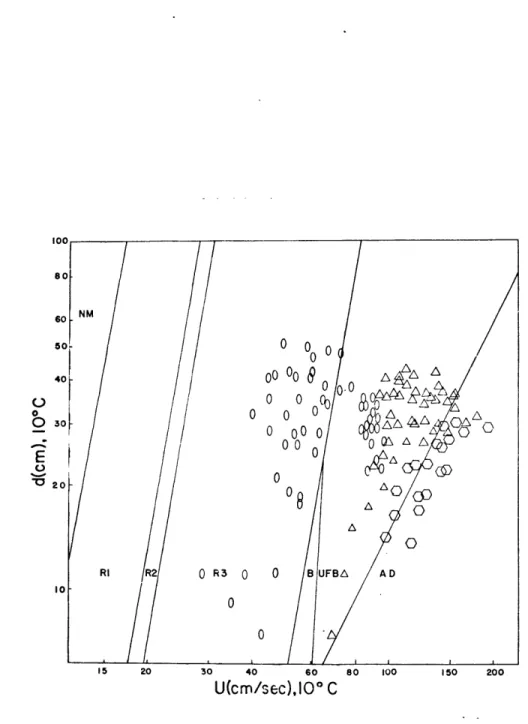
The correlation between the set of fundamental variables and bed phases can be portrayed graphically. There is only one dimensional analysis of the set of fundamental variables that both permits the explicit expression of the environmental determinants in a correlative plot as well as reduces the num-ber of dimensionless parameters characterizing bed configura-tions to three rather than four. That analysis, first pro-posed by Southard (1971), yields the following dimensionless parameters:

d 1/3 D(g1/3 UL)1/3 ps 31

Specifying quartz-density sand and constant-temperature water makes the fourth parameter a constant. Reduction to

- 53

-three parameters permits visualization of the complete one-to-one correlation of the specifying parameters with bed phase or a dependent variable in a three-dimensional diagram essentially contoured for the fourth variable. Specifying constant water temperature (gravitational acceleration is constant) makes all the nondimensionalizing coefficients

con-stant, so that the independent parameters associated with the axes of the diagram are mean flow depth, mean flow velocity, and median sediment size. These explicit environmental de-terminants are easier to interpret sedimentologically than dimensionless parameters.

In this diagram, each data point is uniquely associated with a bed phase. Points of like bed phase are grouped into bed-phase stability fields, which define the range of con-ditions over which a bed phase is stable. Bed-phase stability

fields are separated by boundaries, which seem to be narrow regions of gradational rather than sharp change.

The depth-velocity-size diagram has been used as a guide to investigation and as a framework for organizing data for laboratory studies (Southard and Boguchwal, 1973; Costello, 1974) and for field studies (Jackson, 1975; Dalrymple, 1976). However, in Southard's original presentation (1971) and in these above studies, data were plotted without regard to

temperature. Recognition that data were actually imprecisely plotted forms the basis of discussion for the remainder of Part III.

Objectives.

Establishment of dynamic scale modeling for bed configu-rations is germane to the depth-velocity-size diagram in two ways. The first, underlying the discussion above, is

veri-fication that the fundamental variables on which the diagram is based comprise the entire fundamental set of variables. The second is that in order to meet the criterion of a

constant-temperature plot, the dynamic equivalent of a sys-tem to one at a standard sys-temperature can be determined using

Eq (1.8) for dynamic similitude. (Eq (1.9) is unnecessary

for this purpose since, for quartz-density sand, p s/p is

essentially constant over the whole range of water tempera-tures.)

Eq (1.8) can be used to illustrate the effect of

dis-regarding temperature in a plot of data within an explicitly dimensional depth-velocity-size diagram. For example, taking

two data points, one measured at 5*C and the other measured at 27*C, the length scale relative to one another is 1.5.

By not plotting the dynamic equivalent of one of the points

(to the temperature of the other), the sediment size and depth for that point are off by a factor of 1.5 and the

velocity by a factor of about 1.22, a significant disparity. The plot of a point relative to a standard temperature is therefore shifted considerably as compared to a plot of that point relative to its observed temperature. Hence, for plots in two of the three dimensions of the depth-velocity-size

- 55

-diagram, the net result of adhering to the criterion of a standard temperature would be a wholly different combination of data points per plot than would appear using nonrigorous plotting techniques.

The primary objective of Part III was to construct a three-dimensional depth-velocity-size diagram from existing flume data, taken from other studies, in such a way that data measured at different temperatures could be compared. If the data are plotted dimensionlessly, the effect of

temperature is accounted for by the kinematic viscosity, which appears in each of the first three parameters in Eq

(3.1). However, it is worth preserving the dimensional

property of the diagram, which makes the diagram much easier to comprehend, interpret, and apply than as if it were

dimensionless.

At the same time that data were normalized for tempera-ture, observations of bed configurations were re-evaluated, since in the new synthesis of the data, new and different comparisons of observations would likely be made. Observa-tions were re-evaluated according to the hierarchy of bed forms observed at a particular set of conditions; hierarchy here denotes that bed forms are elements of which the

con-figuration as a whole is composed. This approach was taken for increased resolution in the conception of bed phase.

CONSTRUCTION OF DIAGRAMS

Temperature normalization of data.

Data for the depth-velocity-size diagram were taken from those sources that documented temperature as well as mean flow depth, mean flow velocity, and median grain size for each run; an adequate description of.the bed configura-tion was an addiconfigura-tional requirement of a source, so that observations could be meaningfully re-evaluated. Sources used and the approximate range of normalized sediment sizes for each appear in Table 3.1.

There are two equivalent ways of preserving the dimen-sionality of the data: plot data in dimensionless form and relabel the axes in accordance with a standard temperature, or plot data already normalized to a standard temperature. The first approach was used to plot the data; however, data were normalized before being plotted in order to determine at what constant intervals two-dimensional plots of the three-dimensional diagram could be made, a procedure des-cribed in the next section.

Normalization of the data or of the coordinates of the axes for temperature is determined by Eq (3.2) below. P is the value of a dimensionless parameter, either as calculated

from the data or as read from one of the axes, C is the.value of the non-dimensionalizing coefficient of that parameter at

the standard temperature, and L is the unknown temperature equivalent and multiplicand of that particular coefficient: