HAL Id: hal-00317650
https://hal.archives-ouvertes.fr/hal-00317650
Submitted on 30 Mar 2005
HAL is a multi-disciplinary open access
archive for the deposit and dissemination of
sci-entific research documents, whether they are
pub-lished or not. The documents may come from
teaching and research institutions in France or
abroad, or from public or private research centers.
L’archive ouverte pluridisciplinaire HAL, est
destinée au dépôt et à la diffusion de documents
scientifiques de niveau recherche, publiés ou non,
émanant des établissements d’enseignement et de
recherche français ou étrangers, des laboratoires
publics ou privés.
Large-scale velocity fluctuations in polar solar wind
B. Bavassano, R. Bruno, R. d’Amicis
To cite this version:
B. Bavassano, R. Bruno, R. d’Amicis. Large-scale velocity fluctuations in polar solar wind. Annales
Geophysicae, European Geosciences Union, 2005, 23 (3), pp.1025-1031. �hal-00317650�
© European Geosciences Union 2005
Geophysicae
Large-scale velocity fluctuations in polar solar wind
B. Bavassano, R. Bruno, and R. D’AmicisIstituto di Fisica dello Spazio Interplanetario (C.N.R.), Roma, Italy
Received: 21 May 2004 – Revised: 10 December 2004 – Accepted: 15 December 2004 – Published: 30 March 2005
Abstract. The 3-D structure of the solar wind varies
dra-matically along the Sun’s activity cycle. In the present paper we focus on some properties of the polar solar wind. This is a fast, teneous, and steady flow (as compared to low-latitude conditions) that fills the high-latitude heliosphere at low solar activity. The polar wind has been extensively investigated by Ulysses, the first spacecraft to perform in-situ measurements in the high-latitude heliosphere. Though the polar wind is quite a uniform flow, fluctuations in its velocity do not appear negligible. A simple way to characterize the solar wind struc-ture is that of performing a multi-scale statistical analysis of the wind velocity differences. The occurrence frequency dis-tributions of velocity differences at time lags from 1 to 1024 h and the corresponding values of mean, standard deviation, skewness, and kurtosis have been obtained. A comparison with previous results in ecliptic wind at both low and high solar activity has been performed. It comes out that the kind of trend observed in the distributions for changing scale is the same for the different solar wind regimes. Differences between different flows just have an effect on the values of the distribution moments and the scales at which the transi-tion from non-Gaussian to Gaussian-like behaviours occurs. This is typical of systems in which random fluctuations are mixed to coherent structures of some characteristic size, in other words, systems where long-range correlations cannot be neglected.
Keywords. Heliosphere (Solar wind plasma; Sources of the
solar wind) – Space plasma physics (Turbulence)
1 Introduction
Plasma measurements by Ulysses during its first out-of-ecliptic orbit (started after Jupiter’s gravity assist in Febru-ary 1992) have provided the first in-situ observations of the high-latitude solar wind. Two full orbits have now been completed (third aphelion on June 2004), covering an en-tire solar activity cycle. The data show that the 3-D struc-ture of the solar wind varied dramatically over the solar cycle
Correspondence to: B. Bavassano
(e.g. McComas et al., 2003). Throughout the first orbit, in a period of low solar activity, the solar wind displayed quite a simple bimodal structure, with a persistently fast, tenuous and uniform solar wind at high heliographic latitudes (the so-called polar wind) and slower, more variable, and highly structured wind at low latitudes (e.g. McComas et al., 1998, 2000). In sharp contrast, around solar maximum variable flows were observed at all latitudes and the wind structure appeared to be a complicated mixture of flows coming from a variety of sources (McComas et al., 2002a, 2002b, 2003; Neugebauer et al., 2002). However, as highlighted by Mc-Comas et al. (2002b), this situation persists for a relatively short phase at high solar activity, whereas the remainder of the cycle appears dominated by a solar wind with bimodal structure.
A simple method to characterize the solar wind structure is that of looking at the statistical properties of the wind ve-locity variations at various scales. Under this perspective, multi-scale statistical analyses of velocity differences have been recently performed by Burlaga and Forman (2002) and Burlaga et al. (2003) for the ecliptic solar wind. The first study refers to observations at 1 AU for both low and high so-lar activity, using Wind and ACE data during 1995 and 1999, respectively. The second one focuses on the radial evolu-tion, by both applying a model for solar wind expansion and comparing to Voyager 2 data. Regarding the out-of-ecliptic solar wind, a comparison between wind velocity variations in high-latitude and in ecliptic solar wind for solar maximum conditions has been performed by Bavassano et al. (2004). The polar solar wind is the only wind regime not yet investi-gated through a multi-scale statistical analysis. Though polar wind is quite a uniform flow, fluctuations in its velocity mag-nitude V are not negligible (e.g., see Neugebauer et al. (1995) on high-latitude microstreams). Thus, a multiscale analysis of the V variations in polar wind appears as a useful tool to improve our understanding of this kind of plasma flow. This is the goal of the present study. We will analyse large-scale variations, defined (Burlaga, 1984) as those appearing in time profiles of hourly averages for intervals of several solar rota-tions (or, in terms of spectral analysis, periods roughly from a few hours to a solar rotation).
1026 B. Bavassano et al.: Large-scale velocity fluctuations in polar solar wind 300 500 700 900 (km/s)
V
S N 2 6 10 (cm-3 )N
1 3 5 (AU)R
l l l l l ll l l l l ll l l ll l l ll l l ll l l l SR Sr Nr NR 1993 1994 1995 1996 1997 -60o 0o 60oyear
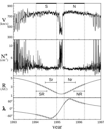
l l l l ll l l l l l lll lll l l l l l ll l l l lFig. 1. From top to bottom, daily averages of the solar wind
veloc-ity V , of the proton number densveloc-ity N∗(normalized to 1 AU), and
of the Ulysses heliocentric distance R and heliographic latitude λ are plotted versus time for years 1993 to 1996. Thick bars on top and dashed vertical lines highlight the analysed intervals during the south (S) and north (N) polar pass of the first out-of-ecliptic orbit. See text for further details.
2 Data and method of analysis
Solar wind measurements by the SWOOPS plasma ana-lyzer aboard the Ulysses spacecraft (principal investigator D. J. McComas) have been used in the present analysis. From the individual velocity vectors, at a time resolution of 4 or 8 min, depending on the mode of operation, hourly averages of the magnitude V of the solar wind velocity have been com-puted. Our study is based on these hourly values.
An overview of the period under investigation is shown in Fig. 1. Here daily averages of the wind velocity V (in km/s), the proton number density N∗(in cm−3, normalized to 1 as-tronomical unit assuming an inverse square scaling with dis-tance), and the spacecraft coordinates (heliocentric distance
R, in astronomical units, and heliographic latitude λ, in de-grees) are plotted versus time for years 1993 to 1996, cover-ing both southern and northern polar phases of the first out-of-ecliptic orbit. Thick bars in the top panel and dashed verti-cal lines indicate the investigated intervals (S and N) from the southern and northern pass, respectively. Each interval cor-responds to a high-latitude cut of the Ulysses orbit for a time length of thirteen solar rotations (as seen by the spacecraft). Solar rotations are shown in Fig. 1 by vertical ticks along the
Rand λ curves. Due to the asymmetry between the northern
Table 1. The analysed data intervals: start and end times (year, day,
hour), minimum and maximum distances (R, in AU), and latitudes
(λ, in◦, with n and s for north and south, respectively).
inter- time R λ
val min max min max
S 94 015 05 – 94 356 05 1.61 – 3.76 49.7 s – 80.2 s N 95 118 12 – 96 094 22 1.44 – 3.59 41.3 n – 80.2 n SR 94 015 05 – 94 194 10 2.72 – 3.76 49.7 s – 72.7 s Sr 94 168 12 – 94 356 05 1.61 – 2.89 49.7 s – 80.2 s Nr 95 118 12 – 95 306 20 1.44 – 2.67 41.3 n – 80.2 n NR 95 281 01 – 96 094 22 2.50 – 3.59 41.3 n – 68.2 n
and southern orbital leg, the same time length does not cor-respond to the same latitudinal range in the two hemispheres. In fact, in the Northern (Southern) Hemisphere 13 rotations correspond to latitudes poleward of 41.3◦(49.7◦). To look for the presence of radial trends, the N and S intervals have been further divided into 2 subintervals of 7 rotations each, referring to the inner and outer portion of the investigated in-tervals. They are indicated by segments drawn in the R panel and labelled Nr and Sr (north and south inner regions) and NR and SR (north and south outer regions), respectively. Ob-viously, latitude changes as well with radial distance along the Ulysses trajectory, however, the latitudinal excursions in the inner and outer intervals are not strongly different, thus variations, if any, should be mainly due to radial effects. The beginning and end times of these intervals, together with their distance and latitude ranges, are given in Table 1. It is worth noting that there is a partial overlapping between the inner and the outer intervals.
As shown by Fig. 1, in the selected intervals the so-lar wind velocity (top panel) is varying between ∼700 and
∼800 km/s. These variations are much smaller than those typically observed in the ecliptic wind (for instance, see in the figure the large V variations during the low-latitude pass of Ulysses at the beginning of 1995). However, polar wind variations do not appear negligible. Though weak, at large enough distances they can lead to appreciable effects. As al-ready noticed by previous studies (e.g. Horbury and Balogh, 2001), at the time of Ulysses observations the southern wind velocity was more modulated by corotating features than the northern one, especially in the outer region. This is very well highlighted by the north-south difference seen in the
N∗panel for sharp density enhancements, typically built up by compression effects at velocity gradients.
The multi-scale statistical analysis of the velocity varia-tions is based on 1) the computation of velocity differences at different time lags and 2) the evaluation of statistical quan-tities for the resulting ensembles (e.g. see Burlaga and For-man, 2002). Thus, starting from the time series of V hourly averages, we have first derived a set of time series of velocity differences dV n(t ) at time lags τ =2n(in hours) as
for n= 0, 1, 2, ..., 10. Then, for each of the eleven dV n en-sembles, the occurrence frequency distribution and the corre-sponding values of mean, standard deviation, skewness, and kurtosis have been computed. All this provides an overview of the basic features of the solar wind velocity structure at scales from 1 to 1024 h (or, 0.0417 to 42.7 days). The choice of 10 as an upper value for n is done to avoid a strong fall of the size of the dV n ensemble. With a number of hourly averages for each of the analysed intervals (Nr, NR, Sr, and SR) in the range 4300–4500, at n=10 the number of data has dropped to ∼76% of that at n=0. If n=11 is used, this per-centage abruptly decreases to ∼53%.
As is well known, the skewness, the third moment nor-malized to the second moment raised to 3/2, measures the asymmetry of a distribution, and the kurtosis, the fourth mo-ment normalized to the squared second momo-ment, measures its peakedness (relative to a Gaussian distribution). For a Gaussian distribution the skewness is obviously 0, while the kurtosis has a value of 3. The definition used here gives an unbiased estimate of the kurtosis (essentially with subtrac-tion of the factor 3), then in the present paper the kurtosis is 0 for a Gaussian distribution. In the following we will refer to these quantities as moments of a distribution, though they are not directly the moments but rather ratios between the moments. Note that some authors call flatness the ratio of the fourth moment to the squared second moment and define kurtosis as flatness –3. A caveat about kurtosis in in order. Though widely used as a measure of non-Gaussianity, kurto-sis has some drawbacks when estimated from measured sam-ples (Hyv¨arinen and Oja, 2000). The main problem is that it can be very sensitive to outliers (Huber, 1985), in other words the value of kurtosis may depend on only a few observations in the tails of the distribution, which might be erroneous or irrelevant observations.
In addition to this kind of analysis, we have also computed power spectra of the V fluctuations to obtain an overview of the scaling regime(s) and look for periodicities in the data. This has been made separately for the four intervals analysed (Nr, NR, Sr, and SR). In the following sections we will first examine the results of this spectral analysis, then we will fo-cus on the distributions of the velocity differences and their moments.
3 Power spectral density of the velocity fluctuations
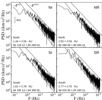
The power spectral density (PSD) of the velocity fluctuations has been computed by using an FFT algorithm on intervals of 4096 hourly averages (i.e. 170.67 days in time). These in-tervals, slightly shorter than the four selected inin-tervals, have been chosen in such a way as to cover the innermost portion of Nr and Sr and the outermost portion of NR and SR, respec-tively. The results of the spectral analysis are shown in Fig. 2, where, for sake of simplicity, we use the labels Nr, NR, Sr, and SR, though the time intervals to which the FFT analysis has been applied are not exactly coincident with those of Ta-ble 1. For each panel the exact radial range and time interval
104 105 106 107 108 109 PSD ((km/s) 2/Hz) 95 118 12 95 289 04 North 1.44 2.55 AU Nr 80% ~F2 ~F5/3 95 289 06 96 094 22 North 2.55 3.59 AU NR 10-7 10-6 10-5 10-4 104 105 106 107 108 109 F (Hz) PSD ((km/s) 2/Hz) 94 185 13 94 356 05 South 1.61 2.78 AU Sr 10-7 10-6 10-5 10-4 F (Hz) 94 015 05 94 185 21 South 2.77 3.76 AU SR
Fig. 2. Power spectral density (PSD) of the velocity fluctuations
versus the frequency F . Panels Nr and NR (Sr and SR) are for the inner and outer region of the northern (southern) polar wind, respec-tively. Radial range and time interval are indicated in each panel.
Straight lines are drawn to indicate the F−5/3and F−2scalings.
An 80% confidence bar is shown in panel Nr.
are given at the bottom. A 3-pt smoothing procedure has been applied to the spectral estimates. An 80% confidence interval is shown in panel Nr.
Though similar in shape, the spectra of Fig. 2 exhibit dif-ferences in several respects. Apart from the lowest and the highest frequencies, the spectra appear well bounded by the
F−5/3and F−2power laws. As is well known, the first cor-responds to Kolmogorov’s scaling for hydrodynamic turbu-lence in the inertial range, while the second is generally un-derstood as a scaling due to a series of discontinuities. It is difficult to obtain a general conclusion about a favourite scaling with frequency. For instance, the Nr spectrum seems closer to F−5/3, while F−2seems better for the SR spectrum. The high-frequency flattening observed for all the spectra is almost certainly related to instrumental sensitivity effects. Regarding low frequencies, the SR spectrum is characterized by the presence of peaks near and below 10−6Hz, that may be associated with solar rotation effects. In fact, for this in-terval the average duration of a solar rotation is 25.6 days, which corresponds to a frequency of 4.5×10⁻⁷Hz. The largest peak in the SR spectrum is just around this frequency, and two other major peaks appear as harmonics of the so-lar rotation frequency. All this is not surprising. Figure 1 clearly shows that a residual modulation in the wind veloc-ity is present for a major fraction of the SR interval, a high-latitude remnant of the corotating velocity structures seen during 1993 by Ulysses.
1028 B. Bavassano et al.: Large-scale velocity fluctuations in polar solar wind 0.1 1 10 NR/Nr PSD ratio SR/Sr 10-7 10-6 10-5 10-4 0.1 1 10 Nr/Sr F (Hz) PSD ratio 10-7 10-6 10-5 10-4 NR/SR F (Hz)
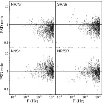
Fig. 3. Power density ratios are plotted to compare results in the
analysed intervals. The upper panels refer to radial variations in the same hemisphere, while a comparison between the two hemi-spheres, for approximately the same radial range, is performed in the lower panels.
The level of power spectra in Fig. 2 appears to decrease when going from the inner (Nr and Sr) to the outer (NR and SR) portion of the analysed intervals. As mentioned above, since the latitudinal excursion of the inner and outer inter-vals is almost the same, the observed power decline should be only due to a radial effect. To obtain an overall compar-ison between the power levels in the four different intervals we plot in Fig. 3 their mutual ratios. The upper panels refer to radial variations in the same hemisphere, while a comparison between the two hemispheres, for approximately the same radial range, is performed in the lower panels. The radial de-crease just mentioned is clearly apparent in the ratios plotted in the upper panels, with values generally below unity (es-pecially at North). Regarding the North-South differences, in the inner region the northern wind velocity seems slightly more variable than that of the corresponding southern wind. No clear trend comes out in the outer region. All this primar-ily holds for the core of the investigated frequency range. An example of a departure from these trends is the strong pres-ence of solar rotation effects in the SR interval, as already discussed above.
4 Statistics of the velocity differences
The velocity differences dV 1, dV 2, dV 4, and dV 6 (at time lags of 2, 4, 16, and 64 h, respectively) are plotted versus time in Fig. 4 (second to fifth panel from top) for a period of one solar rotation. The V hourly averages from which the velocity differences have been derived are shown in the
700 750 800 850 (km/s) V -40 0 40 (km/s) dV1 2-hr -40 0 40 (km/s) dV2 4-hr -40 0 40 (km/s)dV4 16-hr 200 205 210 215 220 225 -40 0 40 (km/s) day of year (1995) dV6 64-hr
Fig. 4. Solar wind velocity V and velocity differences dV 1, dV 2,
dV4, and dV 6 for a solar rotation at the top of the Ulysses’ northern
pass.
top panel. The selected interval is the fourth of the in-vestigated solar rotations in the Northern Hemisphere (see Fig. 1), that encloses the highest latitudes (λ above ∼79◦)
of the Ulysses polar pass. The plotted set of curves clearly shows how at small scale the velocity differences have a rela-tively small amplitude and a turbulence-like appearance (e.g. see dV 1 panel), while at large scale (e.g. dV 6 panel) large-amplitude variations resembling the original V pattern are observed.
Histograms of the velocity differences dV 0, dV 1, dV 2,
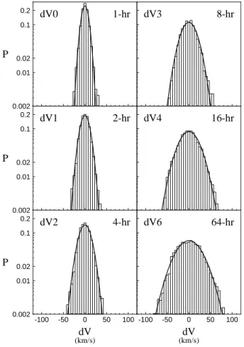
dV3, dV 4, and dV 6 (for time lags of 1, 2, 4, 8, 16, and 64 h, respectively) are shown in the panels of Fig. 5. P is the occurrence frequency, namely the number of cases falling within each bin normalized to the total number. The bin width is 5 km/s for all the scales. The curves drawn in each panel are Gaussian distribution functions computed by using the observed values of mean and standard deviation (in other words, they are not the result of a fit procedure). It is clearly seen that the distribution width increases when going towards longer lags. At a first glance the histograms appear exempt from strong non-Gaussian features.
A quantitative characterization of the dV n frequency dis-tributions can be obtained by evaluating their moments (or
0.002 0.01 0.02 0.1 0.2 P dV0 1-hr dV3 8-hr 0.002 0.01 0.02 0.1 0.2 P dV1 2-hr dV4 16-hr -100 -50 0 50 100 0.002 0.01 0.02 0.1 0.2 (km/s) dV P dV2 4-hr -100 -50 0 50 100 (km/s) dV dV6 64-hr
Fig. 5. The occurrence frequency P (in a logarithmic scale) of the
velocity differences dV 0, dV 1, dV 2, dV 3, dV 4, and dV 6 is shown by histograms in the different panels. The solid curves correspond to Gaussian distribution functions as computed from the observed values of mean and standard deviation.
moment-related parameters). In Fig. 6 the dependence upon
τ of mean, standard deviation, skewness, and kurtosis is shown separately for the four (Nr, NR, Sr, and SR) in-vestigated intervals. Regarding the mean (top panel), its value is seen to remain close to zero for all intervals up to
τ=128 h, then departures come out (that in some cases may be a nonnegligible fraction of the corresponding standard de-viation). The standard deviation (second panel from top) roughly ranges from 5 to 45 km/s. For all the analysed in-tervals the standard deviation increases with τ for lags below 128 h, then becomes nearly constant. These plateau levels are higher for the southern intervals, especially at large distance (see the SR curve). Finally, the values of skewness and kurto-sis (third and fourth panel, respectively) clearly indicate that the statistics is different at different scale, with non-Gaussian distributions (i.e. departures from zero of skewness and/or kurtosis) at small lags and close-to-Gaussian distributions (i.e. nearly zero skewness and kurtosis) at large lags. This holds for all the examined intervals. The transition between the two kinds of distribution roughly occurs in the 16- to 32-h
τrange. The largest departures from a Gaussian are observed
-20 -10 0 10 20 Mean (km/s) Nr NR Sr SR 10 20 30 40 St. Dev. (km/s) -0.6 -0.3 0 0.3 0.6 Skewness 1 2 4 8 16 32 64 128 256 512 1024 0 1 2 (hours) Kurtosis
Fig. 6. The dependence of mean, standard deviation, skewness, and
kurtosis on the time lag τ is shown separately for the four (Nr, NR, Sr, and SR) Ulysses intervals.
in the SR interval where, as already mentioned, the wind ve-locity exhibits a residual modulation by corotating structures. Regarding the caveat given in Sect. 2 about kurtosis, a careful inspection of the data used in the analysis allows us to be confident that the observed kurtosis behaviour does not derive from erroneous or irrelevant data.
5 Discussion and conclusion
The 3-D structure of the solar wind is strongly dependent upon the phase of the solar activity cycle. The present study focuses on some properties of the polar solar wind. This is a fast, teneous, and relatively steady flow that, with ex-clusion of a rather short phase at high solar activity, is a dominant feature of the high-latitude heliosphere. Though small, fluctuations in the polar wind velocity cannot be con-sidered negligible. In the present paper we have studied these fluctuations by using a multi-scale statistical analysis of the velocity differences at time scales from 1 to 1024 h. This kind of technique has already been applied to ecliptic solar wind (Burlaga and Forman, 2002; Burlaga et al., 2003) and to high-latitude solar wind at solar maximum (Bavassano et al., 2004). In addition to this analysis, a classical tool such as
1030 B. Bavassano et al.: Large-scale velocity fluctuations in polar solar wind power spectrum computation has been used in order to obtain
an overview on scaling regimes and look for periodicities in the velocity data. In the following we will first discuss the spectral analysis results, then we will focus on the distribu-tions of the velocity differences and their moments.
A comparison between our spectra (Fig. 2) and those ob-tained by Burlaga and Forman (2002) for ecliptic solar wind indicates that for frequencies above roughly 10−5Hz the level of the velocity fluctuations is lower (of about one or-der of magnitude) in polar wind, though the spectral shape is similar. It must be noted, however, that polar observations re-fer to larger distances and that in the analysis of Burlaga and Forman (2002) the radial component of the solar wind ve-locity was used, instead of the veve-locity magnitude (as done here). At frequencies below 10−5Hz the differences become more relevant. In fact, contrary to ecliptic wind spectra, po-lar wind spectra tend to flatten when approaching frequen-cies close to 10−6Hz (with the exception of the SR inter-val, already discussed above). This spectral range, as high-lighted by Burlaga and Forman (2002), reflects variations as-sociated with the stream structure. It is not surprising that this frequency band appears depleted in polar wind. Finally, around and below 10−6Hz the ecliptic spectra are dominated by peaks introduced by long-living (more than one solar ro-tation) structures rotating with the Sun. These peaks are ab-sent in the polar wind, with the exception of the SR interval, where the solar modulation still has non-negligible effects.
Let us examine now the multi-scale analysis results, in particular the distribution moments and their variation with scale, or time lag τ . We have found that 1) the mean val-ues of the distributions remain close to zero up to τ =128 h, then departures from zero come out, 2) the standard devi-ation increases with τ for lags below 128 h, then becomes nearly constant, 3) the values of skewness and kurtosis show that non-Gaussian distributions are typical of the small lags, while close-to-Gaussian distributions are generally observed at large lags, and 4) the transition between these two kinds of distribution roughly occurs in the 16- to 32-h τ range.
When these results are compared to those by Burlaga and Forman (2002) for ecliptic wind at both high and low so-lar activity, it clearly appears that the overall trend is simi-lar but with relevant differences in the values of the parame-ters (note that no comparison is possible for the distribution means, since they have not been reported by those authors). In all cases the standard deviation of dV n distributions first increases with τ and then remains nearly constant. However, in the polar wind the standard deviation is notably lower than in the ecliptic wind. This simply reflects the fact that the po-lar wind is a much less variable flow than that observed at low latitudes. Regarding skewness and kurtosis, in all cases we have non-Gaussian distributions at small lags and Gaussian-like distributions at large lags. However, the departure from a Gaussian behaviour at small scales is much less pronounced for polar wind. For instance, for τ =2 h, in the polar wind we find kurtosis values between roughly 1 and 2, while for ecliptic wind values as high as ∼16 near solar maximum and
∼7 near solar minimum are observed. Moreover, in the polar
wind the Gaussian behaviour is established at smaller scales (roughly 1 day) than in the ecliptic wind (3 or more days). It is worth mentioning that our results agree very well, in terms of both scales and amplitudes, with those by Neuge-bauer et al. (1995) on the presence of microstreams in the polar wind.
In conclusion, the kind of trend observed in the dV n distri-bution moments for changing scale is the same for different solar wind regimes as 1) the ecliptic wind near solar max-imum, dominated by transient flows related to solar distur-bances, 2) the ecliptic wind near solar minimum, dominated by fast streams from equatorward expansions of polar coro-nal holes, and 3) the polar wind, an almost steady flow from polar solar regions. The differences between flow regimes have rather the effect of leading to different values of 1) the distribution moments, and 2) the scales at which the transi-tion from non-Gaussian to Gaussian-like behaviours occurs. All this is reminiscent of systems in which random fluctu-ations are mixed to coherent structures of some character-istic size (e.g. Bruno et al., 2003a, 2003b, 2004), in other words, systems in which long-range correlations cannot be neglected. In our case the wind velocity pattern represents the structure on which fluctuations, probably related to tur-bulent processes, are superposed.
Acknowledgements. The use of data from the Ulysses/SWOOPS
plasma analyzer (principal investigator D. J. McComas, Southwest Research Institute, San Antonio, Texas, USA) is gratefully ac-knowledged. The data have been obtained through the NASA World Data Center A for Rockets and Satellites (Goddard Space Flight Center, Greenbelt, Maryland, USA). We are indebted to G. Con-solini for very fruitful discussions. The present work has been sup-ported by the Italian Space Agency (ASI) under contract IR/064.
Topical Editor R. Forsyth thanks R. Skoug for his help in eval-uating this paper.
References
Bavassano, B., D’Amicis, R., and Bruno, R.: Solar wind velocity at solar maximum: A search for latitudinal effects, Ann. Geophys., 22, 3721–3727, 2004,
SRef-ID: 1432-0576/ag/2004-22-3721.
Bruno, R., Carbone, V., Sorriso-Valvo, L., and
Bavas-sano, B.: Radial evolution of solar wind intermittency in
the inner heliosphere, J. Geophys. Res., 108(A3), 1130, doi:10.1029/2002JA009615, 2003a.
Bruno, R., Carbone, V., Sorriso-Valvo, L., and Bavassano, B.: On the role of coherent and stochastic fluctuations in the evolving solar wind MHD turbulence: Intermittency, Proceedings of So-lar Wind 10 Conference, edited by: Velli, M., Bruno, R., and Malara, F., American Institute of Physics Conference Proceed-ings 679, p. 453, doi:10.1063/1.1618632, 2003b.
Bruno, R., Sorriso-Valvo, L., Carbone, V., and Bavassano, B.: A possible truncated-L´evy-flight statistics recovered from in-terplanetary solar-wind velocity and magnetic-field fluctuations, Europhys. Lett., 66, 146, doi:10.1209/epl/i2003-10154-7, 2004. Burlaga, L F.: MHD processes in the outer heliosphere, Space Sci.
Burlaga, L. F. and Forman, M. A.: Large-scale speed fluctuations at 1 AU on scales from 1 hour to ≈1 year: 1999 and 1995, J. Geo-phys. Res., 107(A11), 1403, doi:10.1029/2002JA009271, 2002. Burlaga, L. F., Wang, C., Richardson, J. D., and Ness, N. F.:
Evolution of the multiscale statistical properties of corotating streams from 1 to 95 AU, J. Geophys. Res., 108(A7), 1305, doi:10.1029/2003JA009841, 2003.
Horbury, T. S. and Balogh, A.: Evolution of magnetic field fluc-tuations in high-speed solar wind streams: Ulysses and Helios observations, J. Geophys. Res., 106, 15 929–15 940, 2001. Huber, P.: Projection pursuit, Ann. Statistics, 13, 435–442, 1985. Hyv¨arinen, A. and Oja, E.: Independent component analysis:
algo-rithms and applications, Neural Networks, 13, 411–431, 2000. McComas, D. J., Bame, S. J., Barraclough, B. L., Feldman, W. C.,
Funsten, H. O., Gosling, J. T., Riley, P., Skoug, R., Balogh, A., Forsyth, R., Goldstein, B. E., and Neugebauer, M.: Ulysses re-turn to the slow solar wind, Geophys. Res. Lett., 25, 1–4, 1998. McComas, D. J., Barraclough, B. L., Funsten, H. O., Gosling, J.
T., Santiago-Mu˜noz, E., Skoug, R. M., Goldstein, B. E., Neuge-bauer, M., Riley, P., and Balogh, A., Solar wind observations over Ulysses first full polar orbit, J. Geophys. Res., 105, 10 419– 10 433, 2000.
McComas, D. J., Elliot, H. A., and von Steiger, R.: Solar wind from high-latitude coronal holes at solar maximum, Geophys. Res. Lett., 29(9), doi:10.1029/2001GL013940, 2002a.
McComas, D. J., Elliot, H. A., Gosling, J. T., Reisenfeld, D. B., Skoug, R. M., Goldstein, B. E., Neugebauer, M., and Balogh, A.: Ulysses’ second fast-latitude scan: Complexity near solar maximum and the reformation of polar coronal holes, Geophys. Res. Lett., 29(9), doi:10.1029/2001GL014164, 2002b.
McComas, D. J., Elliott, H. A., Schwadron, N. A., Gosling, J. T., Skoug, R. M., and Goldstein, B. E.: The three-dimensional solar wind around solar maximum, Geophys. Res. Lett., 30(10), 1517, doi:10.1029/2003GL017136, 2003.
Neugebauer, M., Goldstein, B. E., McComas, D. J., Suess, S. T., and Balogh, A.: Ulysses observations of microstreams in the solar wind from coronal holes, J. Geophys. Res., 100, 23 389–23 395, 1995.
Neugebauer, M., Liewer, P. C., Smith, E. J., Skoug, R. M.,
and Zurbuchen, T. H.: Sources of the solar wind at
so-lar activity maximum, J. Geophys. Res., 107(A12), 1488, doi:10.1029/2001JA000306, 2002.