A determination of air-sea gas exchange and upper ocean biological production from five noble gasses and tritiugenic helium-3

A Determination of Air-Sea Gas Exchange and Upper Ocean Biological

Production From Five Noble Gases and Tritiugenic Helium-3

by

Rachel H. R. Stanley

B.S. Massachusetts Institute of Technology, 2000

Submitted in partial fulfillment of the requirements for the degree of Doctor of Philosophy

at the

MASSACHUSETTS INSTITUTE OF TECHNOLOGY

and the

WOODS HOLE OCEANOGRAPHIC INSTITUTION

September, 2007

© Rachel H.R. Stanley, MMVII. All rights reserved.

The author hereby grants to MIT and WHOI permission to reproduce paper and electronic copies

of this thesis in whole or in part and to distribute them publicly.

MASSACHUsE OFTEO

OCT 2

LIB

Signature of Author

...

...

Joint Program in Chemical Oceandraphy

Massachusetts Institute of Technology

and Woods Hole Ocea

graphic

Institution

/'y

August 10, 2007

Certified by...

Dr.

iiam J. Jenkins

D*

r." W-

'illiam J.

i i I

i

Jenkins

Senior Scientist

Thesis Supervisor

A ccepted by

...

Dr. Timothy I. Eglinton

INOtOGY Chair, Joint Committee for Chemical Oceanography

Senior Scientist

2

2007

ARIES

A Determination of Air-Sea Gas Exchange and Upper Ocean Biological Production from

Five Noble Gases and Tritiugenic Helium-3

by

Rachel H. R. Stanley

Submitted to the Department of Marine Chemistry and Geochemistry, Massachusetts Institute of Technology-Woods Hole Oceanographic Institution,

Joint Program in Chemical Oceanography on August 10, 2007, in partial fulfillment of the

requirements for the degree of Doctor of Philosophy

Abstract

The five noble gases (helium, neon, argon, krypton, and xenon) are biologically and chemically inert, mak-ing them ideal oceanographic tracers. Additionally, the noble gases have a wide range of solubilities and molecular diffusivities, and thus respond differently to physical forcing. Tritium, an isotope of hydrogen, is useful in tandem with its daughter helium-3 as a tracer for water mass ages. In this thesis, a fourteen month time-series of the five noble gases, helium-3 and tritium was measured at the Bermuda Atlantic Time-series

Study (BATS) site. The time-series of five noble gases was used to develop a parameterization of air-sea gas exchange for oligotrophic waters and wind speeds between 0 and 13 m s- 1 _{that explicitly includes bubble}

processes and that constrains diffusive gas exchange to ± 6% and complete and partial air injection pro-cesses to ± 15%. Additionally, the parameterization is based on weeks to seasonal time scales, matching the time scales of many relevant biogeochemical cycles. The time-series of helium isotopes, tritium, argon, and oxygen was used to constrain upper ocean biological production. Specifically, the helium flux gauge tech-nique was used to estimate new production, apparent oxygen utilization rates were used to quantify export production, and euphotic zone seasonal cycles of oxygen and argon were used to determine net community production. The concurrent use of these three methods allows examination of the relationship between the types of production and begins to address a number of apparent inconsistencies in the elemental budgets of carbon, oxygen, and nitrogen.

Thesis Supervisor: William Jenkins

Acknowledgments

I received funding towards my graduate research from the Department of Defense (NDSEG fellowship), the National Science Foundation (OCE-0221247), and the Scurlock Fund for research.

I would like to give a hundred thank yous to many people who have helped and supported me throughout my time here. First, I feel very lucky for having the opportunity of working with Bill Jenkins. Bill is an amazing advisor, a brilliant scientist and a genuinely wonderful person. Bill's advice, ideas, optimism, and good sense of humor have made the last six years so pleasurable. I sincerely thank my committee members Scott Doney, Jim Ledwell, and Paola Rizzoli. Scott spent an enormous amount of time with me discussing all the scientific questions raised in this study and teaching me how to poke and prod my model. I thank Jim for his thoughtful discussions on air-sea gas exchange and for his encouragement. Paola always made committee meetings a delight and asked very informative questions. Thanks also to Ed Boyle, my thesis defense chair. I am very grateful that Ed read my thesis and came to WHOI to chair my defense.

This work would not have been possible without Dempsey Lott. I am so thankful for Dempsey's exper-tise in building the mass spectrometer, and also for his patience in teaching me so much, for the care he has lavished on me, for his friendship, and for his very kind way of making me feel that eventually we would solve all our problems. I also thank past and present members of the Helium Isotope Lab for wonderful times and lots of help: Josh Curtice, Kevin Cahill, Burkard Baschek, Carolyn Walker, Zoe Howard-Bond, and Angela Landolfi. I am very grateful for the support and encouragement that Mark Kurz and Dave Glover have given to me throughout all of graduate school. I thank DeDe Toole and Naomi Levine for their friendship and support and also for the use of their computers for running my models.

I thank the WHOI Academic Programs Office for taking such good care of me and of all of us graduate students. It was always lovely to stop by the office and receive such a warm welcome. The administrative staff of the Marine Chemistry and Geochemistry department have been very helpful to me. I especially thank Donna and Sheila for helping me with forms and posters and room reservations and for always giving a smile and a warm word as well as the necessary signature or computer work.

I am grateful for the technical skill and dedication of Paul Keith, who not only welded many of the parts of the mass spectrometer so expertly, but who did it so kindly and quickly that it was always a pleasure to visit the welding shop. I also thank Charlie Clemshaw and Rich Zuks for their skill and hardwork.

My time here at WHOI has been enriched by the wonderful friendships I have made. The sometimes overwhelming task of writing a thesis was made possible thanks to the support and encouragement from many of my friends who were going through the same process themselves. I thank Clare, Anna, Jessica and Carlos for sharing these last few months of thesis writing frenzy. I thank Rose for her great support and encouragement - knowing I had a friend on the first floor made the evenings in my office pass quickly. I thank Nick for being one of my biggest and most special supporters throughout all of graduate school. And I thank Carolyn for sharing so much - an office, an advisor, a house, and so many wonderful times. I also thank my friends from before graduate school who have cheered me on for the last six years: Anna, Danielle, Laurie, Amanda, Liz, Karen, and Pascale.

I am grateful for all the support and encouragement that my family has lavished on me. I especially thank my father Gene for his care and advice and my brother Michael for his frequent pep talks. I sincerely thank my husband Dwight for giving me so much, advising me on science and math problems, encouraging me when nothing was working, and celebrating with me when things went well. The long days at work passed quickly because I knew that Dwight would be there for me when I finally went home.

In the interest of brevity, I give a final thank you to all my friends and colleagues. I do not have space here to thank each one individually but all have enriched my life for which I am sincerely grateful.

Dedication

This thesis is dedicated to the memory of my mother, Idahlia Stanley. She was an amazing

woman, a creative thinker, an inspired painter, and a wonderful mother. She taught me to ask

questions and to give reasons. Her memory gives me courage and inspiration to tackle tough

Contents

1 Introduction

1.1 M otivation. ... . . . .. . . . ... . . .. . . . .. . . 1.2 Overview of Approach . . . . 1.3 Chapter by Chapter Plan . . . . 2 A Method for Measuring Five Noble Gases and Their Isotopic Ratios Using Stainless Steel Cryogenic Trapping and a Combination of Quadrupole and Magnetic Sector Mass Spectrom-eters

2.1 Introduction . . . . 2.2 M ethods . . . . . . ... . .. . . .. .

2.2.1 Method for a gas standard ...

2.2.2 Additional Steps for a Water Sample .. . .... . . . ... . . . . ... . . . 2.2.3 Details of QMS Analysis ... ...

2.2.4 Details of Magnetic Sector Analysis ... . . . .... . .. ... . . . 2.2.5 Computer Control ...

2.2.6 Standardization ... .. .. . ... .. . . . ... . . . 2.3 Analytical Performance and Reproducibility . . . . 2.3.1 Performance of the QMS and Processing Line ... . . . .. . . . .. . . . . . 2.3.2 Performance of the HIMS for He Isotopes . ... . . . ... . . . ... 2.4 Discussion ... ... ... ... .. ...

2.4.1 Separation of the Noble Gases ... ... 2.4.2 Matrix Effects of Ar and Xe on Kr ...

2.4.3 Hydrogen ... ... ... . .... 30 31 32 38 40 40 41

44

2.4.4 Methane ... 68

2.4.5 Error Analysis ... 69

2.5 Conclusions ... 72

2.6 Acknowledgments ... . 73

3 Quantifying Seasonal Air-Sea Gas Exchange Processes Using Noble Gas Time-Series: A De-sign Experiment 75 3.1 Introduction ... 77

3.2 Methods ... 78

3.2.1 Description of the one-dimensional vertical upper ocean model: Physical parameters 78 3.2.2 Description of the model: Gas exchange parameters . ... 81

3.2.3 Linearization and inverse technique ... ... 85

3.3 Choice of physical parameters ... 87

3.4 Sensitivity Study: Constraints on air-sea gas exchange parameters from the noble gases . . . 89

3.4.1 Model results: Noble gas behavior ... ... 89

3.4.2 Quantifying the constraints ... 94

3.5 Example application: Time-series of helium, neon, and argon . ... 99

3.6 Conclusions ... 108

3.7 Acknowledgments ... 110

4 Air-Sea Gas Exchange Parameters as Determined by a Time-Series of Five Noble Gases 113 4.1 Introduction ... ... ... 115

4.2 Methods ... 117

4.2.1 Data Collection ... ... 117

4.2.2 Description of the one-dimensional vertical upper ocean model . ... 121

4.2.3 Gas exchange parameterization used in the model . ... . . . 123

4.2.4 Inverse Method ... ... 126

4.3 Results . . . .. .. . . . ... .128

4.3.1 Noble Gas Data ... ... 128

4.3.2 Inverse Model Results ... ... 132

4.4.1 The Base Case ... 4.4.2 Controls on the Parameters 4.4.3 Sensitivity of Parameters . Conclusions ... Acknowledgments . . . . 138 146 147 153 156

5 Estimates of Biological Production from a Time-Series of Noble Gases, Tritium, and Helium-3157

5.1 Introduction ... 159

5.2 M ethods ...

5.2.1 Data Collection . ... 5.2.2 He Flux Gauge Calculations ...

5.2.3 Apparent Oxygen Utilization Rate Calculations 5.2.4 Oxygen and Argon Time-Series Calculations . 5.3 Results and Discussion . ...

5.3.1 He Flux Gauge ...

5.3.2 Apparent Oxygen Utilization Rates ... 5.3.3 Oxygen and Argon Time-Series ... 5.4 Synthesis ... 5.5 Conclusions ... ... 162 162 165 167 170 173 173 184 193 200 204 5.6 Acknowledgments ... .. .. .. ... .. .. .. .. ... .. .. .. ... .206 6 Conclusions and Future Directions

...

. . . .

. . . .

List of Figures

1-1 Solubilities and diffusivities of the noble gases . . . . Schematic of the processing line and mass spectrometers. ...

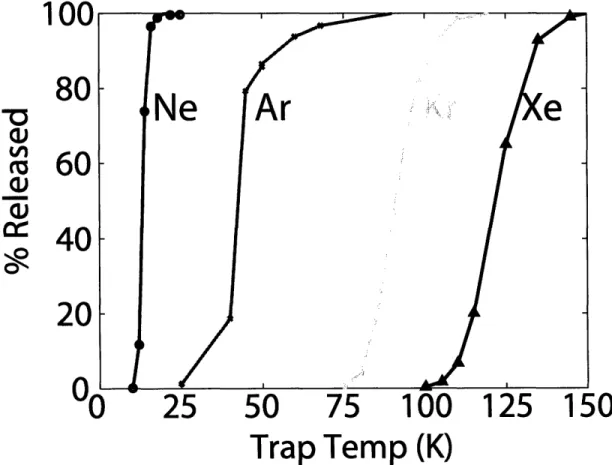
Temperature cycles of the stainless steel cryotrap . ...

Release curves of the noble gases from the stainless steel cryotrap. ... Inlet curves for the noble gases into the QMS. ... . . Peak shapes for the noble gases as measured by the QMS. ...

Peak shapes for the noble gases at various cage voltages. ...

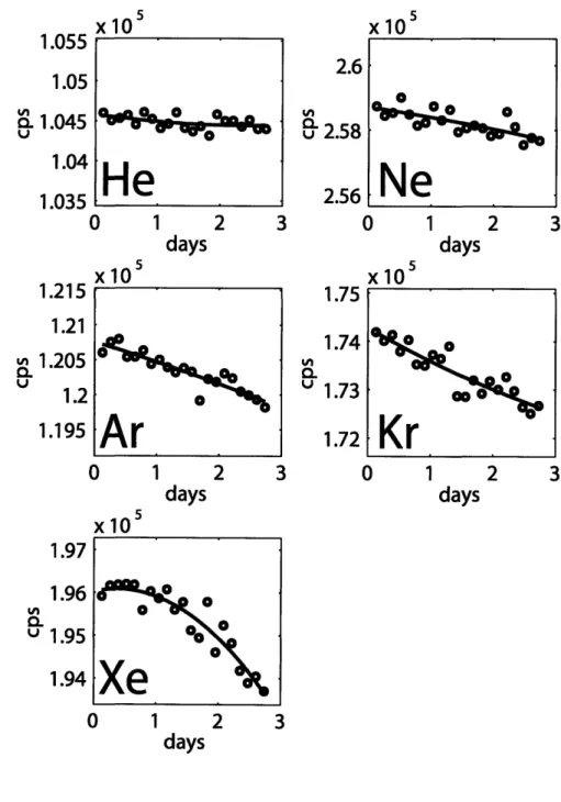
Repeated QMS measurements on standards over several days . . . . . Deviations of repeated QMS measurements of standards. ...

. . . . . 33 . . . . . 34 . . . . . 48 . . . . . 50 . . . . . 53 . . . . . 54 . . . . . 57 . . . . . 58

2-9 Peak shapes for He and HD as measured on the magnetic sector mass spectrometer ... 60

2-10 Matrix effects on the stainless steel cryotrap. . ... ... 66

3-1 Comparison of temperature and salinity between model and BATS/Station S data ... 88

3-2 Surface saturation anomalies for the five noble gases and oxygen as predicted by the model . 90 3-3 Saturation anomalies in the top 300 m for the five noble gases as predicted by the model .. 91

3-4 Xe surface saturation anomaly for model runs with different gas exchange parameters . . .. 93

3-5 Linearization of observational metric as a function of model parameter ... 96

3-6 Time-Series of He, Ne, Ar data from 1989 ... 101

3-7 Modeled diffusive gas exchange, total air injection, and partial air injection fluxes for He, Ar,andX e. . . . .. . . .. . .. . .. . . . . .. . . . .. . . .. . . 106

4-1 Upper ocean saturation anomalies of the five noble gases: data and model ... 129

4-2 Upper ocean concentrations of the five noble gases: data and model . ... 130 2-1 2-2 2-3 2-4 2-5 2-6 2-7 2-8

Surface saturation anomalies of the five noble gases ... . . . 131

Vertical profiles of observed saturation anomalies for He and Ne . ... 133

Vertical profiles of saturation anomalies for Ar, Kr and Xe . ... 134

Upper ocean temperature from BATS data and as predicted by model . ... 140

Model-data differences of saturation anomalies and concentrations of the noble gases . . . . 141

Modeled fluxes of the noble gases ... 143

Inventories of the noble gases in the upper 160 m in the base case model and from the data . 145 Sensitivity of the noble gases to the proportion of complete to partial trapping. ... 148

Comparison of solubility values ... 151

5-1 Box model for predictions for tritium, 3He, and T/He age as a function of replacement time . 169 5-2 Vertical profile of productivity in model 5-3 5-4 5-5 5-6 5-7 5-8 5-9 5-10 5-11 5-12 5-13 . . . .. 172

Seasonal modulation of productivity profile in model ... .. 174

j3He isotope ratios, gas transfer velocity, and fluxes ... ... 176

Relationship between

6

Change in correlation of 3He and NO with time ... .... 181

Effect of air injection on equilibrium 63He ... 183

Time-series of tritium and excess 3He ... 186

Profile of ventilation replacement time r ... ... 187

Profiles of apparent oxygen utilization rate ... ... 189

Difference in saturation anomaly of 02 and Ar in model and data . ... 194

Difference in saturation anomalies of 02 and Ar in the mixed layer . ... 197

Sensitivity study to seasonal amplitude of production . . ... .. . . 198

6-1 Profile of the noble gases to 4200 m depth ... 213 4-3 4-4 4-5 4-6 4-7 4-8 4-9 4-10 4-11

List of Tables

2.1 Theoretical and experimentally determined amount of gas left behind in a sample bulb . . . 2.2 Parameters used by the QMS to measure the five noble gases in a water sample or gas standard. 2.3 Measurement details for He, Ne and Ar ...

2.4 Measurement details for Kr and Xe ...

2.5 Amount of gas in one aliquot of each type of gas standard . ...

2.6 Performance of the QMS for measuring the major isotopes of the five noble gases... 2.7 Linearity of the QMS measurements ...

2.8 Performance of the QMS for distilled water samples . ... ... 2.9 Coefficients for matrix effect on Kr ...

2.10 Sources of errors in the measurements of the noble gases. . ... Reference case values for tunable gas exchange parameters ...

Uncertainties on model parameters from the partial derivative method . . . 3.3 Constrains on parameters from the full inverse method ... . . 3.4 Observational metrics in example application . ...

3.5 The slope matrix in the example application . ... 3.6 Model parameter values for the example application ...

3.7 Appendix: Definition of symbols and variables . . . . 4.1 Details of sample collection. ...

4.2 Contribution of bubbles entrained in samples during collection ... 4.3 The three best sets of physical parameters ...

4.4 Magnitudes of contributions to ao ...

4.5 The air-sea gas exchange parameters as determined by the inverse modeling .

. . . . . 86 . . . . .. 95 . . . . . 97 . . . . .102 . . . . .103 . . . . ... 104 . . . .111 .. .. .... 120 . . . . . 121 .. .. .. ..123 ... . .... 127 . . . . . ... 135

4.6 The corresponding fluxes as determined by the inverse modeling . ... 136

4.7 The air injection fluxes of the sum of the major gases as determined by the inverse modeling 137 4.8 The contributions of complete vs. partial trapping ... .... 138

4.9 The sensitivity of the parameters to the exclusion of different gases . ... 147

5.1 Regression between 63Heex and NO in the thermocline . ... 177

5.2 Estimates of biological production from this study ... .... 179

5.3 Estimates of export production in different depth regions of the water column ... 190

5.4 Net community production as estimated from euphotic zone seasonal cycles of 02 and Ar .. 195

Chapter 1

1.1 Motivation

The ocean plays a key role in the biogeochemical cycle of many climatically relevant gases such as CO2,

CH4, N20, etc. These gases are at historically unprecedented levels in today's atmosphere (e.g. Keeling

et al., 1996; Petit et al., 1999; Fluckiger et al., 1999; Spahni et al., 2005) and thus the exchange of gas between the atmosphere and the ocean is of particular importance. The ocean is a significant sink for anthropogenic CO2 (Siegenthaler and Sarmiento, 1993; Cox et al., 2000) but exactly how CO2 is sequestered

and how this amount will change with time is not well understood. For example, recent evidence suggests that the Southern ocean sink of CO2 is becoming saturated (Le Quer~ et al., 2007). Other gases than CO2 also

have potentially varying sources and sinks in the ocean. The primary natural sources of N20 are emission

from ocean upwelling regions and from tropical soils. Since the magnitude and location of denitrification may change with climate, the oceanic source of N20 may change as well. Another climatically relevant gas,

DMS, is produced in the ocean and diffuses into the atmosphere, where through the CLAW hypothesis it

may participate in important climate feedbacks (Charlson et al., 1987).

All gases in the atmosphere and ocean cross the air-sea boundary and thus are affected by air-sea gas

exchange. The challenge is that air-sea gas exchange is a complicated, dynamical physical problem which is very difficult to measure directly. Thus bulk parameterizations of air-sea gas exchange flux have been developed to allow researchers to calculate the net result of air-sea gas exchange for a given gas in a given condition (Liss and Merlivat, 1986; Wanninkhof, 1992; Wanninkhof and McGillis, 1999; Nightingale et al., 2000). Recent studies suggest that these earlier estimates may be too large by approximately 20% to 30% (Ho et al., 2006; Sweeney et al., 2007). These air-sea flux relationships are important for global climate change models as well as for flux calculations. For example, bulk parameterizations have been used in conjunction with maps of surface seawater pCO2 to infer air-sea CO2 fluxes for different regions of the

ocean (Takahashi et al., 1997). Additionally, quantification of air-sea gas exchange fluxes is necessary for biogeochemical research that uses gases as tracers to investigate key problems. For example, 02/N2 ratios

in the atmosphere can be used to infer partitioning of CO2 between land and ocean sinks (e.g. Keeling et al.,

1993; McKinley et al., 2003; Bender et al., 2005) and 02 measurements in the ocean can be used to infer net community production (e.g. Jenkins and Goldman, 1985; Craig and Hayward, 1987; Emerson, 1987). One sign of the ubiquity of use of these air-sea gas exchange parameterizations is that the most commonly used

parameterization by Wanninkhof (1992) has been cited 890 times.

Existing parameterizations, however, have uncertainties of 25 to 50%, leading to uncertainties that prop-agate through all studies using these parameterizations. Depending on the parameterization used, global and regional fluxes can differ by up to 100% (Fangohr and Woolf, 2007). Additionally existing parameterizations are based on either short time-scales of hours to days or on long time-scales such as decades. The shortest time scales are assessed by micrometeorological techniques (Wanninkhof and McGillis, 1999) which have time scales of hours. Radon deficit calculations (Peng et al., 1979) and deliberate dual release experiments (Watson et al., 1991) allow prediction of gas exchange paramterizations on time scales of several days to two weeks. In line with the short time scales, these estimates are necessarily local in scope. At the other extreme, gas exchange parameterizations estimated from natural or bomb radiocarbon budget have decadal or longer time scales (Broecker and Peng, 1974; Wanninkhof, 1992; Sweeney et al., 2007). Such estimates are by nature global in scope. Yet it is the intermediate time scale of weeks to seasonal that matches the time scale of many biogeochemical processes in the ocean.

Moreover, most existing parameterizations do not explicitly treat bubbles. Air injection (the flux due to bubbles) is a complicated problem of bubble dynamics (e.g. Memery and Merlivat, 1985; Woolf and Thorpe, 1991; Woolf, 1993; Keeling, 1993; Woolf et al., 2007). The air injection flux can be significant, especially for less soluble gases such as 02 and He. Finally, the techniques that determine air-sea gas exchange parameters from direct empirical data, such as purposeful release experiments, are logistically difficult and have only been applied in limited areas of the ocean. The major goal of this thesis is therefore to determine an air-sea gas exchange parameterization with uncertainties of only 10 to 20% that is based on direct, emprical data, that explicitly includes bubbles, and that is based on weeks to seasonal time-scales.

Another reason for studying gases in the ocean is that gases can be used to constrain upper ocean bio-geochemical cycles. Understanding the carbon cycle is key for climate research since CO2 is an important

greenhouse gas. As mentioned above, CO₂ enters the ocean through air-sea gas exchange. Marine organ-isms then fix approximately 50 Pg of carbon per year (Field et al., 1998). Some of this organic matter is remineralized in the surface of the ocean and thus has no net effect on CO2 concentrations. Some of it,

however, is exported into deep water and separated from the atmosphere on time scales of hundreds of years. The importance of biological production in the ocean has long been known. Standard techniques for

measuring biological production include bottle experiments in which radiotracers are added to bottles of seawater which are then incubated and analyzed. While such experiments are useful, they have limitations due to so-called "bottle effects" produced by confining production to a single bottle, eliminating grazers, trace metal contamination from the bottles, etc. Additionally, bottle experiments offer only a snap-shot of production at one particular place and time. Sediment traps quantify export production and offer the advantage of direct collection of sinking material. However, hydrodynamic biases and swimmers make sediment trap data difficult to interpret (Gardner, 2000). Newly designed neutrally-buoyant sediment traps (Buesseler et al., 2000; Valdes and Price, 2000; Stanley et al., 2004; Buesseler et al., 2007) avoid some of these problems but nonetheless sediment traps, as well as bottle experiments, may miss episodic events (such as production stimulated by eddies) which may constitute a large fraction of production (McGillicuddy et al., 2007).

Geochemical tracers complement the traditional approaches to estimating production because they char-acterize the integrated behavior of systems over broad spatial and temporal scales. A variety of geochemical tracers have been used to quantify three types of production -net community production (e.g. Jenkins and Goldman, 1985; Craig and Hayward, 1987; Spitzer and Jenkins, 1989; Gruber et al., 1998), export produc-tion (e.g. Jenkins, 1980; Sarmiento et al., 1990), and new producproduc-tion (Jenkins, 1988b; Jenkins and Doney, 2003). Net community production is defined as primary production minus heterotrophic respiration. New production is defined as the production stemming from input of new nutrients into the euphotic zone (Dug-dale and Goering, 1967). Over sufficiently long temporal and spatial scales, the three types of production should be equal (Eppley and Peterson, 1979). In this study, I use geochemical tracers to measure all three types of production at the same location and at the same time for an in-depth analysis of the carbon cycle in a subtropical oligotrophic gyre. By using all these methods concurrently, I examine the relationship between the types of production and begin to address a number of apparent inconsistencies in the elemental budgets of carbon, oxygen, and nitrogen.

1.2 Overview of Approach

1. To provide a quantitatively more accurate parameterization of air-sea gas exchange rates that explicitly includes bubble-mediated processes on biogeochemically relevant time scales

2. To use three tracer subsystems in order to concurrently quantify new, net community, and export production in an oligotrophic subtropical gyre.

In order to achieve these objectives, I have collected a monthly time-series of five noble gases (He, Ne, Ar, Kr, and Xe), helium isotopes and tritium at the Bermuda Atlantic Time-series Study (BATS) site. I then combine this data with a one dimensional, vertical, modified Price-Weller-Pinkel (PWP) model (Price et al., 1986; Spitzer and Jenkins, 1989) in order to separate and quantify gas exchange parameters. By combining the noble gas and tritium data with biogeochemically active constituents, such as NO and 02, I also constrain biological production.

Noble gases are ideal tracers because they are biologically and chemically inert and thus respond solely to physical forcing. Additionally, there are five of them with a range of solubilities and molecular diffusiv-ities (Figure 1-1). The diffusivdiffusiv-ities differ by a factor of five with helium being the most diffusive (J'ihne et al., 1987). The solubilities differ by a factor of ten, with xenon being the most soluble (Wood and Caputi, 1966; Weiss, 1971; Weiss and Kyser, 1978; Hamme and Emerson, 2004b). Additionally, the solubilities of the heavier noble gases have a stronger dependence on temperature. This broad range in physicochemical characteristics leads to differing response to physical forcing. Thus measurements of multiple noble gases made concurrently allow us to diagnose and quantify physical processes.

Helium (He) and neon (Ne), the lightest gases, are useful because they are insoluble with relatively lit-tle temperature dependence and therefore are sensitive to air injection processes. Krypton (Kr) and Xenon (Xe), the heaviest gases, are useful because they have a strong temperature dependence to solubility and thus respond to thermal forcing. Argon (Ar) is intermediate in behavior and has a solubility and diffusivity very similar to that of molecular oxygen. Thus, it is especially important because it can serve as an abiotic analogue to 02. Oxygen signatures in the ocean are a result of physics and biology. Argon mimics the physics and thus the difference between 02 and Ar can be a tracer for biological productivity (Craig and Hayward, 1987; Emerson, 1987; Spitzer and Jenkins, 1989). In practice, however, the story is more com-plicated since Ar and 02 have different gradients and distributions. In the aphotic zone, 02 is consumed through remineralization, resulting in an 02 debt that is mixed upward. Argon in contrast, has a relatively

Figure 1-1: (a) Molecular diffusivities of the noble gases and oxygen as a function of temperature, as calculated from the diffusivity values of Jiihne et al. (1987). Helium, the lightest noble gas, is more diffusive by a factor of five than Xe, the heaviest noble gas. (b) Solubilities of the five noble gases and oxygen as a function of temperature. The solubilities vary by an order of magnitude, with Xe being the most soluble and having the strongest temperature dependence. Solubility values for He are from a modified version of Weiss (1971), Ne and Ar solubilities are from Hamme and Emerson (2004b), Kr solubility is from Weiss

and Kyser (1978) and Xe solubility is from Wood and Caputi (1966).

(a) Diffusivity

(b) Solubility

Y

10f-9

20

25

Temperature (C)

140

120

T100

E

S80

E 60

40

20

30

15

20

25

Temperature (C)

6

5

4

3

2

15

30

constant saturation anomaly with temperature. By using all the noble gases and a one dimensional model of upper ocean dynamics, I model the physical processes affecting 02 and by difference can estimate biological production.

In previous seawater studies, Ar has been used in conjunction with 02 to estimate biological production (Craig and Hayward, 1987; Spitzer and Jenkins, 1989). Time-series of He, Ne and Ar measurements in seawater have been used to investigate air-sea gas exchange (Spitzer and Jenkins, 1989) as have time-series of Ne, Ar, and N2 (Hamme and Emerson, 2006). Helium measurements in seawater have been used to

investigate escape mechanisms for the exosphere (Bieri et al., 1967). Modeling studies suggest Ar can be used for quantifying diapycnal mixing (Henning et al., 2006; Ito and Deutsch, 2006). The solubility of Kr and Xe have a stronger thermal dependency than Ar and thus these heavier gases allow better constraints on air-sea gas exchange parameters (Stanley et al., 2006) and may be useful tracers of water mass formation processes (Hamme and Severinghaus, 2007).

As part of our time-series, I also measure 3He and tritium. 3He in the ocean has two sources - primordial

3

He from hydrothermal and volcanic activity and 3_{He produced from in-situ tritium decay. In the upper}

ocean at BATS, the main source of 3He is tritium decay (Jenkins, 1980). Tritium is naturally produced in small amounts from cosmogenic rays, but the natural inventory was dwarfed by input of tritium from the thermonuclear bomb tests in the 1950s and 1960s. Tritium was injected into the stratosphere where it formed HTO and then rained out into the ocean. Tritium decays to 3He with a half-life of 12.31 years (MacMahon, 2006) and the combination of tritium and 3He measurements can be used as a "clock" for dating subsurface water (Jenkins and Clarke, 1976). At the surface, the clock is zeroed as most of the 3_{He is fluxed out due}

to gas exchange. As water is subducted and separated from the atmosphere, 3_{He builds up from decay of}

tritium. In practice, mixing complicates this simple scenario but models can be used to calculate ventilation time scales from tritium and 3_{He measurements (Jenkins, 1980; Doney and Jenkins, 1988).}

By measuring a time-series of tritium, 3He, and the noble gases, I am able to resolve the seasonal cycle and build a detailed understanding of the dynamic system. The BATS site is an ideal place for this work for several reasons. First, a time-series of many biogeochemical relevant parameters (but not the noble gases) have been measured at BATS since 1988 (Michaels and Knap, 1996) and before that at Station S since 1954 (Schroeder and Stommel, 1969). Thus there is a wealth of historical data that can be used to constrain the

model and to interpret the results. Second, the infrastructure was in place for sample collection. This not only meant that ship-time was accessible, but also key information such as 02 and nutrient measurements are made as part of the BATS program and ancillary data from the BATS program (such as plankton tows, sediment traps, bottle experiments, etc) may aid in interpretation of results. Third, there is a significant seasonal cycle at BATS, with a summer to winter temperature difference of approximately 10 degrees. Since the heavier noble gases respond most strongly to thermal forcing, a strong temperature cycle causes a supersaturation of the gases in summer, and thus a flux out of the mixed layer which can be parameterized. Fourth, BATS is located in an oligotrophic regime. Ninety percent by area of the oceans are oligotrophic and half of the global carbon export occurs in oligotrophic regimes. Thus a study in such conditions is relevant to much of the world's oceans. Finally, noble gas data at the BATS site is amenable to being modeled with a one-dimensional vertical model. The main factor controlling the distribution of the noble gases is the temperature history of the water. At BATS, the contours of net heat flux parallel the circulation (Worthington, 1976) and thus a one-dimensional model can reasonably be used for the noble gases .

I use a one-dimensional vertical Price-Weller-Pinkel (PWP) (Price et al., 1986) model that has been modified to include He, Ne, and Ar (Spitzer and Jenkins, 1989) and I extend it to the heavier noble gases. I force the model with six-hourly NCEP reanalysis heat flux (Kistler et al., 2001) and with QuikSCAT winds. Modeling is necessary to separate and quantify the physical processes affecting the noble gases. The advantage of a one-dimensional model is that it is simple and transparent. However, a one-dimensional model clearly does not account for horizontal processes and large scale circulation. For reasons described above, the model is sufficient for the noble gases. However, it is not appropriate for use with nutrients, tritiugenic 3He, and tritium because of large scale gyre circulation (Williams and Follows, 1998; Jenkins and Doney, 2003).

1.3 Chapter by Chapter Plan

Noble gases are ideal tracers but the heavier noble gases have not often been measured in seawater, perhaps because they are so difficult to measure. Recent improvements in mass spectrometers, particularly the development of a stainless steel cryogenic trap (Lott, 2001) have made such measurements possible. In Chapter 2 of this thesis, I describe a method I developed for measuring the five noble gases and their isotopes

in seawater samples through mass spectrometry. Automated cryogenic traps are used to first sorb and then to separate the noble gases. Two mass spectrometers are attached to a single processing line, allowing measurements of both helium isotopes and noble gases on the same samples. The noble gases are measured statically by peak height manometry using a quadrupole mass spectrometer, equipped with a pulse-counting secondary electron multiplier. Helium isotopes are measured on a purposely built, branch-tube, statically operated magnetic sector mass spectrometer. Separating the noble gases in a reproducible way can be difficult due to matrix effects of one noble gas on another as well as affects from other gases in seawater (such as methane) and thus great effort was made to reduce and assess matrix effects. Additionally, the mass spectrometer and processing system are precisely standardized, and any effects of nonlinearity are assessed and accounted for. By measuring the noble gases through comparison to precisely known aliquots of air, I avoid using isotope dilution and thus can determine the isotopic ratios of the noble gases in the samples.

In Chapter 3, I perform a modeling sensitivity study in order to determine how well a time-series of five noble gases at BATS could constrain air-sea gas exchange parameters. I extend the PWP model for Kr and Xe and force the model with NCEP reanalysis winds and heat fluxes (Kistler et al., 2001). Ensemble runs are used to optimize tunable physical parameters in order to emulate the temperature, salinity, and mixed layer observations at BATS. I then perform sensitivity studies to characterize the response of the noble gas saturation anomalies to air-sea gas exchange parameters. I use a linear inverse technique (singular value decomposition) in order to determine the constraints offered by a hypothetical time-series of all five gases. As a limited demonstration of the approach, I use a dataset of a time-series of three noble gases (He, Ne, and Ar) collected between 1985 and 1988 in the Sargasso sea (Spitzer, 1989) in order to calculate preliminary estimates of air-sea gas exchange parameters.

In Chapter 4, I present a 14 month time-series of five noble gases collected between July 2004 and August 2005 at 22 depths in the upper 400 m of the ocean. I combine the noble gas data (measured according to the method in Chapter 2) with inverse modeling (as in Chapter 3 but with QuikSCAT winds) in order to develop an air-sea gas exchange parameterization that explicitly includes air injection processes, that has uncertainties of ±6% for diffusive gas exchange and ±15% for air injection over the range of wind speeds encountered in the time-series (0< uIo <13 m s-l), and that provides an estimate on a relevant and unique time scale. I use a nonlinear constrained optimization inverse method and explore the sensitivity of the

parameters to uncertainties in the solubility functions of the noble gases, to uncertainties in the physical parameters used in the model, to the structure of the cost function, and to uncertainties in the model's representations of the gases.

In Chapter 5, I combine the gas exchange parameterization developed in Chapter 4 with 3

He, tritium, 02, and NO3 measurements from the 14 month time-series in order to estimate new, net community, and export production. First, I combine 3He measurements in the mixed layer with the gas exchange parameterization to calculate the 3He flux out of the mixed layer. By correlating 3He in the thermocline with NO3, I can then estimate the flux of NO3 into the mixed layer and the new production flux as it is physically transported by upwelling of thermocline waters. I next use tritium and 3He data from the upper ocean measurements as well as from two profiles that extend to 4200 m depth in order to calculate the ventilation age of the water. I combine apparent oxygen utilization with these ventilation ages to calculate apparent oxygen utilization rates (AOUR). The vertically integrated AOUR is a measure of export production. Finally, I use the euphotic zone seasonal cycles of 02 and Ar with the model developed in Chapters 2 and 3, in order to estimate net community production. This study is unique in that it measures all three types of production using geochemical techniques at the same location and at the same time. By comparing the estimates of the three types of production, I start to examine inconsistencies in the elemental cycling of C, 0, and N.

In summary, this thesis uses the five noble gases as tracers to improve our understanding of air-sea gas exchange processes and upper ocean biological production. The noble gases are used to develop an im-proved parameterization of air-sea gas exchange that explicitly includes bubbles and that can be applied to calculate the air-sea flux of any gas. The noble gases, tritiugenic 3He, and tritium are then used, in conjunc-tion with this improved parameterizaconjunc-tion, to estimate three types of biological producconjunc-tion in a subtropical oligotrophic gyre and to explore the relationship between new, net community, and export production and nutrient cycling.

Chapter 2

A Method for Measuring Five Noble Gases

and Their Isotopic Ratios Using Stainless

Steel Cryogenic Trapping and a

Combination of Quadrupole and Magnetic

Sector Mass Spectrometers

Abstract

A method is presented for precisely measuring all five noble gases and their isotopic ratios in water samples using multiple cryogenic traps in conjunction with quadrupole mass spectrometry and magnetic sector mass spectrometry. Multiple automated cryogenic traps, including a two-stage cryotrap used for removal of water vapor, an activated charcoal cryotrap used for helium separation, and a stainless steel cryotrap used for neon, argon, krypton and xenon separation, allow reproducible gas purification and separation. The precision (expressed as 1 standard deviation) of this method, determined by repeated measurements on gas standards, is +0.10% for He, +0.14% for Ne, +0.10% for Ar, +0.14% for Kr, and +0.17% for Xe. The precision of this method for water samples, determined by measurement of duplicate pairs, is ±1% for He, +0.9 % for Ne, +0.3% for Ar, +0.3% for Kr, and ±0.2% for Xe. Isotopic ratios of the noble gases are measured as well, with precisions of ±0.19% for 20Ne/22Ne, +0.20% for 84Kr/86_Kr,

+0.25% for 84Kr/82Kr, +0.09% for 132Xe/129Xe and +0.13% for 132Xe/136Xe. An attached magnetic sector mass spectrometer measures

2.1 Introduction

Noble gases are biologically and chemically inert and have a wide range of solubilities and diffusivities, making them useful environmental tracers. Noble gases have also been used extensively in groundwater studies to constrain paleotemperatures (Stute et al., 1992, 1995; Aeschbach-Hertig et al., 2000) and ground-water infiltration and recharge (Beyerle et al., 1999; Manning and Solomon, 2003; Zhou et al., 2005). Mea-surements of Ar and Kr isotopes in ice cores can lead to estimation of firn thickness and temperature (Craig and Wiens, 1996; Severinghaus et al., 2001, 2003). Noble gases in mantle-derived rocks have been used to infer properties of the early history of the earth (Honda et al., 1991; Hiyagon et al., 1992; Farley and Neroda, 1998). Noble gas isotopes produced by cosmic rays yield surface exposure ages for terrestrial rocks (Lal, 1991; Bierman, 1994; Schafer et al., 1999).

In seawater studies, noble gas measurements have been used to investigate air-sea gas exchange (Spitzer and Jenkins, 1989; Emerson et al., 1995; Hamme and Emerson, 2006), biological production (Jenkins and Goldman, 1985; Craig and Hayward, 1987), diapycnal mixing (Henning et al., 2006; Ito and Deutsch, 2006), and escape mechanisms for the exosphere (Bieri et al., 1967). Extending the measurements beyond the three noble gases (He, Ne, and Ar) used in previous work allows one to constrain air-sea gas exchange parameters to levels significantly better than can be obtained when only three of the noble gases are used (Stanley et al., 2006). Given that Kr and Xe have a stronger thermal dependency than Ar, the supersaturation pattern of the heavier noble gases may provide probes for ocean mixing and water mass formation processes (Hamme and Severinghaus, 2007). Additionally, the isotopic ratios of the noble gases could be useful tracers.

Quadrupole mass spectrometry (QMS) and magnetic sector mass spectrometry have often been used to measure the noble gases in water samples. Recently, instruments have been developed that measure all five noble gases from a single sample (Poole et al., 1997; Beyerle et al., 2000; Kulongoski and Hilton, 2002; Sano and Takahata, 2005). The analysis is usually conducted by isotope dilution or by peak height comparison with an air standard. The noble gases are commonly chemically purified and then condensed onto a charcoal trap at liquid N2 temperatures (77 K), on a charcoal trap at dry ice/acetone temperature (96K), or on a glass

trap at liquid He (4K). Methods that measure all five gases from a single sample have precisions of 0.3% to 1.0% using magnetic sector instrument (Beyerle et al., 2000) and 0.4% to 1.6% using a QMS system (Sano and Takahata, 2005). Methods that only measure one of the noble gases may have better precisions. For

example, an isotope dilution method for measuring only Ne routinely obtained precisions of 0.13% (Hamme and Emerson, 2004a).

We have developed an automated sample processing and measurement system for the determination of the complete set of noble gas concentrations and isotope ratios in water samples (90 cc) at the 0.1-0.2% level. Active gases are removed from the sample and the remaining noble gases are captured cryogenically and then selectively released for measurement to a quadrupole or a magnetic sector mass spectrometer. We use a set of three cryogenic traps operated in tandem with a Pd catalyst and chemical getters and combined with a volume partitioning system in order to achieve a high degree of purity and separation between the individual noble gases, thereby reducing as much as possible the potential for interference between gas species. The water vapor cryotrap (WVC) is a dual flow through cryotrap with independently controlled temperatures allowing water vapor to be removed but the noble gases to pass unimpeded. The activated charcoal cryotrap (ACC) captures He and then releases an aliquot into the QMS and the remainder into a helium isotope magnetic sector mass spectromer (HIMS) for precise measurements of 3_He/4_{He ratios. A}

"nude" stainless steel cryotrap (SSC) (Lott, 2001) captures Ne, Ar, Kr and Xe and then selectively releases the gases into the QMS. The QMS operates in a static, ion-counting mode which requires a lower partial pressure of gas within the QMS, less gain dependence on the electron multiplier, and a more linear response. Standardization of the system is accomplished using precisely known aliquots of atmospheric noble gases (determined by pressure, temperature, volume and relative humidity), and thus is dependent on knowledge of the abundance of these gases in air. However, since studies involving dissolved gases generally presume these values, uncertainties in these abundances cancel out in most calculations.

2.2 Methods

The sample processing and measurement system is shown in Fig. 2-1. Noble gases from a water sample or gas standard are sequentially drawn through the two-stage WVC to remove water vapor, and through a Pd catalyst and getters for chemical purification, and then onto two cryogenic traps. The AAC at < 10K captures He and then at 40 K releases He into the HIMS. The SSC, also initially at < 10K, captures Ne, Ar, Kr, and Xe and then selectively warms and releases the noble gases (Fig. 2-2) into the statically operated QMS for measurement by peak height manometry. "Static" refers to the sample being let into the isolated

QMS (i.e. no pumping during measurement) and then peak jumping is used to measure the count rates at

each of the pre-determined masses. The QMS is a Hiden quadrupole mass spectrometer (P/N PCI 1000 1.2HAL/3F 1301-9 PIC type 570309), equipped with a pulse counting secondary electron multiplier (SEM) run at an emission of 20 to 40 /-tamps, an electron impact ion source and triple quadrupole ion optics. The HIMS, an improved system based on the "Clarke design", is a purposely constructed branch tube, statically operated, dual collector magnetic sector helium isotope mass spectrometer, radius of 25.4 cm, equipped with a Faraday cup and a pulse counting SEM. The system, including the processing line, cryotraps, and mass spectrometers, is operated under computer program control to achieve a high degree of reproducibility and for continuous operation.

In order to avoid possible systematic biases caused by the interaction between gas species via ion col-lisions and preferential ionization, we use cryogenic techniques to separate the noble gases before they are inlet into the mass spectrometers. Thus each of the noble gases is measured sequentially from the same air standard or water sample. The cryogenic systems used here lead to three cryogenic processes: cryoconden-sation, cryosorption and cryotrapping. Cryocondensation refers to the condensation of gas on a truly inert surface and results in the partial pressure of the gas above the surface being a function only of its vapor pressure at the trap temperature. However, no surface is truly inert, and thus the nature of the surface of the trap influences the amount of gas released. An active surface, such as on the ACC, results in stronger cryosorption and thus releases the gases at higher temperatures than a stainless steel surface such as on the

SSC. For example, Ne is released at 25K on the SSC and at 80K on the AAC.

Cryotrapping refers to one gas being trapped underneath another. Since Ar is three to five orders of magnitude more abundant than the other noble gases, Ar cryotraps the other gases and thus the SSC has to go through many temperature cycles to reproducibly and quantitatively separate and release all the noble gases. In this section, we first outline the process necessary for measuring all five noble gases in a single air standard. Then we discuss some additional particulars that are necessary for processing a water sample.

2.2.1 Method for a gas standard

The processing line is pumped by a diffusion pump, a turbo molecular pump, and three ion pumps (in different parts of the line - see Fig 2-1) to below 5x10- 8 torr before starting an analysis. An aliquot of an air

Figure 2-1: Schematic of the processing line and mass spectrometers (HIMS and QMS) that comprise the analytical system. Red and green squares denote pneumatically actuated copper stem tip (vacuum-type) stainless steel UHV bellows valves (Nupro P/N 22-*BG-TW-CU-3C and SS-4BG-USI-VD-3C), with red squares representing the valves that are closed at the beginning of an analysis and green squares representing the valves that are open at the beginning of an analysis. Valve numbers are included for valves referenced in the text. White squares represent pneumatically operated crackers. Ovals represent aliquot volumes. All aliquots as well as the standard reservoir volumes and the 2 L expansion volume are in an aluminum box in order to keep them at an approximately constant temperature. Purple squares denote pressure gauges with "IG" representing ionization gauges (Granville-Phillips 330), "CV" representing convectron gauges (Granville-Phillips 316), and "MKS" representing a capacitance manometer (MKS baratron PR4000 con-troller with 10 torr type 626A absolute pressure transducer). "IN2 trap" refers to a trap chilled with liquid nitrogen to condense water vapor when initially pumping down the sample bulbs after attaching them to the automanifold - the sample bulbs are still sealed at that point. "Dual WVC" refers to a two-stage cryotrap (inlet and outlet sides) initially held at 160K to trap water in the sample. "AAC" and "SSC" refer to the ac-tivated charcoal and the stainless steel cryotraps respectively. For more detail on the processing line, please refer to the text.

Diffm Fore Pump Pump Air •

I

I

Figure 2-2: Temperature of the stainless steel cryotrap (SSC) as a function of time after analysis has com-menced. The SSC undergoes a number of temperature cycles in order to reproducibly separate and release the noble gases. Gray arrows indicate where gases are released. Black arrows indicate where gases are pumped. Numbers indicate temperatures at various points in the temperature cycles.

3( 2 21 E u tI 0 50 100 150 200

time (minutes)

standard or a sample first passes through the WVC, a two-sided cryotrap held at 160 K, in order to remove water vapor. Then it flows through a Pd catalyst (BASF catalyst R02-20/37) where the CH4 in the standard

is oxidized to CO2 and H20. The pressure is recorded on a capacitance manometer (MKS baratron PR4000

controller with 10 torr type 626A absolute pressure transducer) in order to get a parametric determination of the total gas pressure. The gas then flows through a zirconium-vanadium-iron getter, composed of pellets of STS707 (available from SAES getters) in order to remove active gases. The first half of the getter is heated to 3500C to chemically remove 02, N2, and CO2 and to crack CH4, while the second half of the

getter remains at room temperature (20"C) to sorb H2. The noble gases are inert to the getter pellets and

flow through unimpeded.

The sample is next drawn for 12 minutes onto the SSC, held at less than 9.5 K. Neon, Ar, Kr and Xe are trapped on the stainless steel surface. Helium does not sorb quantitatively to the stainless steel surface at this temperature, so the sample is next exposed for 8 minutes to the ACC (Lott. and Jenkins, 1984) operated at 8.5K in order to trap He. Meanwhile, the SSC is isolated and warmed to 40 K for 3 minutes and then cooled to 9.5 K in order to liberate the 2-4% of the He that was cryotrapped by Ar or the other gases. The ACC subsequently pumps on the SCC for 30 seconds in order to cryosorb this He onto the ACC.

The sample is next drawn for 12 minutes for a second time onto the SSC, while the inlet side of the WVC is warmed to 285 K and the outlet side of the WVC is held at 160 K. The ice is thus melted and the water is distilled onto the outlet WVC, releasing any gases that had been trapped in the ice for subsequent purification and cryotrapping while blocking water vapor.

The SSC is warmed to 60 K and then is cooled back to 25 K in order to outgas and release Ne that had been cryotrapped by Ar. The SSC is then opened and Ne is released from the trap. The amount of Ne released is volumetrically split by a factor of roughly 200 in a reproducible fashion by trapping an aliquot of the released gas between valves 40 and 41 in order to obtain a sample size that gives a counting rate of about 140,000 cps, an optimal counting rate for the SEM, which is operated in the ion counting mode. Too high a counting rate leads to dead-time issues, a nonlinear response, and a short lifetime for the SEM. Too low a counting rate leads to poor Poisson ion-counting statistics. Because volume partitioning is used to split the Ne, some fraction of Ne remains on the SSC. This is removed by ion pumping for 2 minutes at 20 K, which is 5 K less than the release temperature in order to avoid any Ar from being pumped.

The SSC is then warmed to 80 K in order to uniformly distribute Ar on its surface. Meanwhile, the ACC is warmed to 40 K and then is opened to release He. An aliquot of He, equal to approximately 1% of the sample is trapped between valves 38 and 39, is inlet into the QMS, and measured with a counting rate of about 100,000 cps on the SEM. Next, the 99% of the remaining He is volume partitioned into the HIMS where the 3He/4He ratio is measured.

The ACC is then warmed to 80 K. An aliquot of gas is released from ACC and analyzed for Ne, in order to quantify any Ne that did not sorb to the SCC but rather made it through to the ACC. The amount of Ne measured from the ACC is approximately 5% of the amount measured from the SSC for gas standards and approximately 0.5% of the amount measured from the SSC for water samples, suggesting the SSC exhibits a variable Ne trapping efficiency which is dependent on major gas composition, including possibly water vapor. The ACC is cleaned by ion pumping at 80 K for 10 minutes.

Meanwhile, the SSC remains isolated and held at 80 K for two minutes, before it is slowly cooled to

25 K to recondense Ar on the cryotrap. The cooling is slower than usual in order to layer the Kr on the SSC first and then the Ar and thus to minimize commingling of Ar and Kr. The SSC is warmed to 60 K

and opened to release Ar. Because Ar is very abundant in air samples, the Ar sample must be reproducibly split down by roughly a factor of approximately 3x10 6 in order to avoid overwhelming the QMS. Thus Ar is expanded for four minutes into a 2 liter stainless steel expansion volume, through valves 10, 9, 40, 42, 43 and 24. We performed experiments to determine that four minutes were required for the Ar atoms to have time to distribute evenly throughout the expansion volume. When the expansion time was shorter, the Ar signal increased, suggesting that the Ar had not reached equilibrium in the expansion volume, and thus fewer Ar atoms were pumped away, leaving more Ar to be analyzed.

Approximately 0.03% of the Ar is trapped in the aliquot between valves 42 and 43 and the remaining Ar is pumped away using a turbo molecular pump. The Ar in the aliquot is then expanded for a second time, this time into the volume bounded by valves 40, 43, and 9. Again, the Ar in the aliquot between valves 42 and 43 is saved and the rest is pumped away. Once more, the Ar is expanded into the volume bounded

by valves 41, 9 and 43. This time the portion of the Ar in the aliquot between valves 40 and 41 is saved

and inlet into the QMS. Although this splitting procedure may seem cumbersome, it enables the consistent splitting of Ar by a factor of approximately 3x10 6 with a reproducibility of 0.1%.

In order to remove any Ar remaining on the SSC, the SCC is then ion pumped at 62 K for two minutes. This pumping temperature is higher than the release temperature in order to remove enough Ar so as to minimize interference with the Kr measurements. Then, in order to remove any Ar that still remains on the SSC, perhaps cryotrapped under Kr or Xe, a temperature/pumping cycle is performed. The SSC is isolated and warmed to 150 K, cooled back to 62 K, and then ion pumped for 3 minutes. This heating and pumping cycles results in an acceptably low amount of Ar in our Kr and Xe samples - the Ar introduced into the QMS when the Kr is inlet produces an ion current that is about 20% of the Kr signal. It is possible to further reduce the amount of Ar in the Kr inlet by pumping for longer or at higher temperatures. However, this results in significantly greater Kr loss, resulting in deterioration of our Kr results.

The SSC is isolated, warmed to 103 K and opened to release Kr. The Kr is split by a factor of approxi-mately 130 by trapping an aliquot of sample between valves 40 and 41 and then is inlet into the QMS and measured on the SEM at an ion current of approximately 150,000 cps. The SSC is cooled to 93 K and then turbo pumped for 2 minutes to remove remaining Kr. The SSC next undergoes a heating/pumping cycle to remove any Kr cryotrapped by Xe. The SSC is warmed to 150 K, cooled back to 93 K, and pumped on for

1 minute.

The SSC is next warmed to 155 K and opened to release Xe. The Xe is split by a factor of approximately 6 by expansion of the sample through valves 9, 40, 42, and 43 and then trapping of a subsection in the section between valves 9, 41, and 42. This subsection is inlet into the QMS and measured on the SEM with an ion count rate of approximately 150,000 cps. The SSC is turbo pumped for 1.5 minutes to remove any remaining Xe. The SSC is then ion pumped while being warmed to 290 and pumped and held at 290 for five minutes. Next the ACC and the SSC are cooled to 10 K in order to prepare for the next sample.

The total analysis time for one sample is approximately three hours and 20 minutes and the procedure is completely automated. Line blanks are run every few days in order to check for leaks and to assess the cleanliness of the system. Line blanks typically are smaller than 0.004% for He, Kr, and Xe, smaller than 0.01% for Ne, and smaller than 0.07% for Ar.

2.2.2 Additional Steps for a Water Sample

Water samples consist of 90 g of water taken at sea by gravity feeding water from Niskin bottles on a CTD rosette via Tygon tubing into valved stainless steel cylinders. In the on-shore laboratory at the Bermuda Biological Station, we extracted the gases from the cylinders into aluminosilicate glass bulbs (approximate volume of bulb is 25 cc) using the "at-sea extraction system" (Lott and Jenkins, 1998). The glass sample bulb contains >99.95% of the original sample as well as 3 to 5 cc of distilled water transferred during the extraction.

Because He, and to a less extent Ne, permeates through the viton o-rings in the cylinder plug valves, samples were extracted as soon as possible, usually within 24 hours of sample collection. This time period was comparable to the typical delays encountered in practice during the WOCE/CLIVAR sampling. Experi-ments performed with degassed water samples documented the rate at which samples are compromised. He and Ne were equilibrated at rates of 0.46% and 0.09% of their disqulibrium per day. Thus for a sample with a 10% disequilibrium in either He or Ne concentration or He isotope ratio, a 24 hour delay in extraction from the time of sampling would lead to a signal reduction of 0.046%, 0.009%, and 0.046% respectively.

Sets of eight of these glass bulb samples are attached to the automanifold using viton o-ring compression fittings. The manifold is then pumped for at least 2 hours, a processing blank is run to assess for any leaks, and then the samples are individually processed, with one gas standard being run after every two water samples. To process a sample, first all of the sample sections except the sample of interest are closed off, and the manifold is isolated from the vacuum pumps and the rest of the processing line. Custom-fabricated automated "crackers", based on a heavily modified Nupro valve (P/N SS-6-6BK-TW-10), snap the tip of the glass seal-off on the bulb. Experimentation revealed that an optimum pneumatic pressure of 40 psi achieves reliable "cracking open" of the sample. On cracking of the bulb tip, the gas from the headspace of the sample bulb is partitioned into the volume of the manifold.

After 30 seconds, the manifold is opened and the gas expands into the dual WVC. Here, water is drawn out of the sample, quantitatively sweeping all the gas from the headspace out of the bulb into the WVC section of the processing line. After 1.5 minutes, the valve to the bulb is closed to avoid excessive water vapor transfer. Beyond this point, the sample gases are processed in an identical fashion to the standard gases.

Table 2.1: Theoretical and experimentally determined amount of gas typically left behind in a sample bulb after the gas in the headspace is swept into the processing line for analysis. The ratios are different for each position on the manifold. One example set of ratios is listed here. The ratio of theoretical to measured left-behind is used to correct all samples for the total gas in the bulb. Uncertainties in this ratio thus lead to uncertainties in determinations of gas concentrations in samples.

He Ne Ar Kr Xe

Theoretical left-behind (%) 0.16 0.19 0.63 1.1 2.1 Ratio of theoretical to measured left-behind 0.87 0.98 0.79 0.62 0.85 Estimated uncertainty in ratio 0.07 0.1 0.05 0.03 0.03 Uncertainty in final correction for samples (%) 0.01 0.01 0.03 0.01 0.06

Some fraction of the gases are dissolved in water and thus not all the gas is drawn out of the bulb. This amount of gas left behind can be calculated theoretically from the volume and temperature of the water, the volume of the bulb, and the solubility of the gas. Additionally, it was determined experimentally on some samples by repeated drawing of gas from the same sample. More gas was consistently drawn from the samples than the theoretical calculation predicted, suggesting that some of the gas was fluxed out of the water during the draw (Table 2.1). The ratio of the measured sample left behind in the bulb to theoretical sample left behind in the bulb is consistent for each position on the manifold and is used to correct all measurements for the amount of gas left in the bulb. Manifold positions that are closer to the WVC have less gas left-behind because then the WVC is more effective at drawing out the gas. Samples that are on the lower manifold also have less gas left-behind because they are slightly warmed from below by the diffusion pump and gases are less soluble at warmer temperatures. We thus measure the ratio for each position on the manifold and correct each sample accordingly. This ratio is more difficult to calculate for He and Ne since He and Ne diffuse into the bulb during the time period between samples. We used repeated measurements in order to assess the amount of He and Ne that grows in but still our estimates for He and Ne left behinds have larger errors. However, since these gases are the least soluble, only a small percentage is left-behind and thus even with these larger uncertainties, the error added by the total correction is small.