Development and Test of Dynamic Congestion Pricing
Model
by
Shunan Xu
L
Bachelor of Civil Engineering
Tsinghua University, Beijing, P.R. China (2006)
Submitted to the Department of Civil and Environmental Engineering
In partial fulfillment of the requirements for the degree of
Master of Science in Transportation
at the
MASSACHUSETTS INSTITUTE OF TECHNOLOGY
February 2009
@ Massachusetts Institute of Technology 2009. All rights reserved.
CHUSETTS INSTrUE, F TECHNOLOGY
BRAR
2 6 2009
.IEBRARIES
Author ...
...Department of Civil and Environmental Engineering
January
16h,2009
A A A
Certified by ...
Moshe E. Ben-Akiva Edmund K. Turner Professor of Civil and Environmental Engineering Thesis Sypejisor Accepted by ... ...
SDaniele Veneziano
Development and Test of Dynamic Congestion Pricing Model
by
Shunan Xu
Submitted to the Department of Civil and Environmental Engineering
on January
1 6 th,2009, in partial fulfillment of the
requirements for the degree of
Master of Science in Transportation
Abstract
Dynamic congestion pricing is an approach to control the traffic flow on the network
by setting variable tolls that are adjusted with time based on the traffic condition.
Different models have been developed and tested in the past. However, most of these
models are based on deterministic network equilibrium rather than stochastic choices
of travelers, and case studies on complex networks are rare. These disadvantages limit
the use of existing models.
In this research, a new dynamic congestion pricing model is developed based on a
discrete choice framework to capture users' personal choices. Several solution
algorithms are examined and tested in a synthetic network for solving this model.
Among these algorithms, SPSA is found to be the best, and is applied successfully to
a real case study in Lower Westchester County in New York State. The usefulness and
effectiveness of dynamic congestion pricing is also examined and discussed. The
results show that dynamic congestion pricing has the potential to improve network
performance.
Thesis Supervisor: Moshe E. Ben-Akiva
Acknowledgements
It is my great pleasure to have memorable experience in MIT, the top engineering school in the world. The experience enlarges my knowledge, and even more, matures my attitude and mentality towards life and the world. I would like to thank my research advisor Professor Moshe Ben-Akiva for his guidance of my research and study, as well as inspirational presence throughout the course of my work at MIT. I would also like to express my gratitude toward my academic advisor Professor Joseph Sussman for his kind help with my life and courses during my master period, especially in my first year. I am especially thankful my lab-mate Yang Wen for spending so much time to discuss with me the algorithms and the programs.
The Intelligent Transportation System (ITS) lab in MIT is a professional but relaxable place for research and life. Senior members in the lab including Yang Wen, Maya Abou Zeid and Charisma Choudhury are great sources for acquiring helps in courses and research. Vikrant Vaze, Vaibhav Rathi, Varun Ramanujam, Eric Huang, Zheng Wei, Lang Yang, Ying Zhu, Sarvee Diwan and Samiul Hasan are all great co-workers to work with.
I would also like to thank my closest friends Yaoqi Li, Shiyin Hu and Wilson Tam for their encouragements and helps during my master period, as well as all of my friends who made the life in MIT a fantastic experience.
Most importantly I would like to thank my parents, for their understanding and supports to my life from the other end of the world. Finally, thanks to God for providing me such a great journey in MIT.
Contents
1. Introduction ... 11
1.1 Overview of congestion pricing ... ... 12
1.2 Response to congestion pricing... ... 14
1.3 Static and dynamic congestion pricing... 15
1.4 M otivation ... ... ... ... ... 16
1.5 Implemented framework ... ... ... 17
1.6 Contribution ... ... ... ... 18
1.7 O u tlin e... 19
2. Literature Review on Dynamic Congestion Pricing ... 21
2.1 Route choice m odels ... ... ... .... ... 21
2.1.1 Fuzzy logic ... .. . ... ... ... ... 22
2.1.2 Discrete choice model ... ... ... 24
2.2 Departure time choice models...27
2.3 General congestion pricing models ... ... ... ... 30
2.3.1 A nalysis m odel... ... . .. .... ... ... 31
2.3.2 Sim ulation m odel ... .... ... . .... .. ... 32
2.4 Sum m ary ... ... ... ... .... ... 37
3. M odel D evelopm ent ... 39
3.1 Mathematical formulation...39
3.1.1 Optimization formulation structure...40
3.1.2 Formula development... ... 41
3.1.3 Summary of problem formulation...48
3.2 Param eters im plem entation... ... 49
3.2.1 Parameter for the cost in route choice...50
3.2.2 Parameters for early and late arrival penalty... ... 51
3.2.3 Parameters for departure time choice...52
3.3 Summary ... ... ... ... 53
4. Solution Algorithm ... 55
4.1 Characteristics of the dynamic congestion pricing model... ... 55
4 .1.1 L arge scale ... 56
4 .1.2 N on-linearity ... 56
4.1.3 Implicit relationship ... 56
4.2 Overview of optimization algorithms ... 57
4.2.1 Path search methods ... 58
4.2.2 Pattern search methods...67
4.2.3 Random search methods ... 69
5. Assessment of algorithms in synthetic network ... 73
5.1 Case study description ... ... 73
5.1.1 Experiment design...73
5.1.2 Parameter calculation ... 75
5.2 Network equilibrium test ... 77
5.2.1 Introduction to DynaM IT ... 77
5.2.2 Fixed point problems ... 78
5.2.3 Fixed point algorithms for network equilibrium ... ... 79
5.2.4 Tests of fixed point algorithms ... ... 81
5.2.5 Summary of fixed point algorithm ... 87
5.3 SPSA description and test ... 87
5.3.1 Algorithm description... 87
5.3.2 Parameter selection ... 89
5.3.3 SPSA test... 90
5.4 FDSA-M description and test...93
5.4.1 Algorithm description.... ... ... 93
5.4.2 Parameter selection ... ... 96
5.4.3 FDSA-M test ... ... ... 96
5.5 Result analysis ... ... 98
5.5.1 Comparison among different scenarios ... ... 98
5.5.2 Result for the effect of congestion pricing ... 99
5.6 Summary ... 102
6. Case Study: Lower Westchester County ... 103
6.1 Objectives ... ... ... 103
6.2 Case study description ... ... ... 103
6.2.1 Experiment design... 104
6.2.2 Parameter calculation ... 107
6.3 Time convergence algorithm test ... 107
6.4 Result analysis ... ... 108
6.4.1 Case study result ... 109
6.3.2 Usefulness and effectiveness of dynamic congestion pricing ... 110
6.4 Sum m ary ... ... ... 113
7. Conclusion ... ... .. ... ... ... 115
7.1 Summary ... ... ... ... 115
7.2 C ontributions... ... ... 116
7.3 Future research directions ... 117
Appendix A: MATLAB Code for SPSA ... 119
List of Figures
Figure 2.1: Path choice problem ... 24
Figure 3.1: Structure of dynamic congestion pricing model ... ... 43
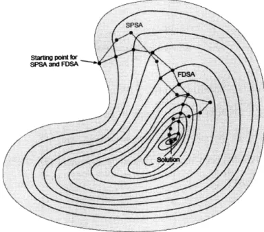
Figure 3.2: Relationship between departure on time probability and cost by different function form s ... 4 5 Figure 4.1: Comparison between the convergence of FDSA and SPSA ... 65
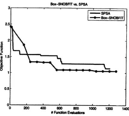
Figure 4.2: Comparison of estimation results for SNOBFIT and SPSA...67
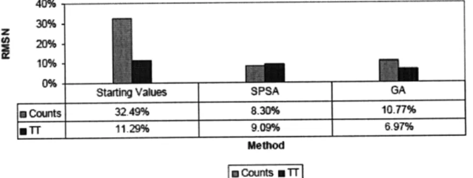
Figure 4.3: Comparison of estimation results for SPSA and GA... ... 71
Figure 5.1: Synthetic network topology...74
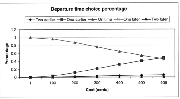
Figure 5.2: Relationship between costs and departure time choices...77
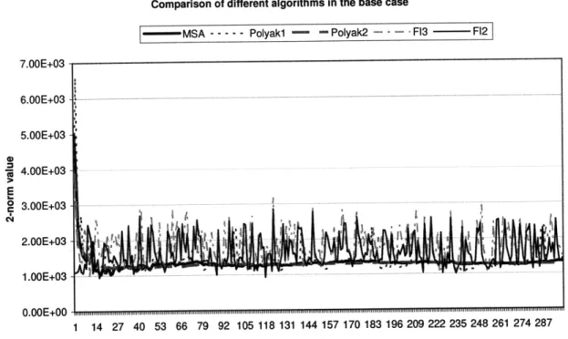
Figure 5.3: Comparison of different algorithms in the base case... ... 83
Figure 5.4: Comparison of MSA and Polyak2 in initial toll scenario ... 84
Figure 5.5: Comparison of MSA and Polyak2 in 15-min flat toll scenario... 85
Figure 5.6: Comparison of MSA and Polyak2 in random toll scenario ... 86
Figure 5.7: SPSA algorithm process ... ... ... 89
Figure 5.8: Result of SPSA for grad_rep= ...1 ... ... 91
Figure 5.9: Result of SPSA for grad_rep=2 ... 91
Figure 5.10: Result of SPSA for grad_rep=3 ... 91
Figure 5.11: FDSA-M algorithm process...94
Figure 5.12: Differences between FDSA and FDSA-M... ... 96
Figure 5.13: Result of FD SA -M ... ... 97
Figure 5.14: Travel time distribution among four scenarios ... 100
Figure 5.15: Departure time distribution for three toll strategies... 100
Figure 6.1: Network of LW C ... ... 105
Figure 6.2: Locations of the toll plazas... 106
Figure 6.3: Results of MSA algorithm in LWC network ... 108
Figure 6.4: Result of FDSA-M application in LWC network ... 109
Figure 6.5: Travel time distribution in three scenarios ... 112
List of Tables
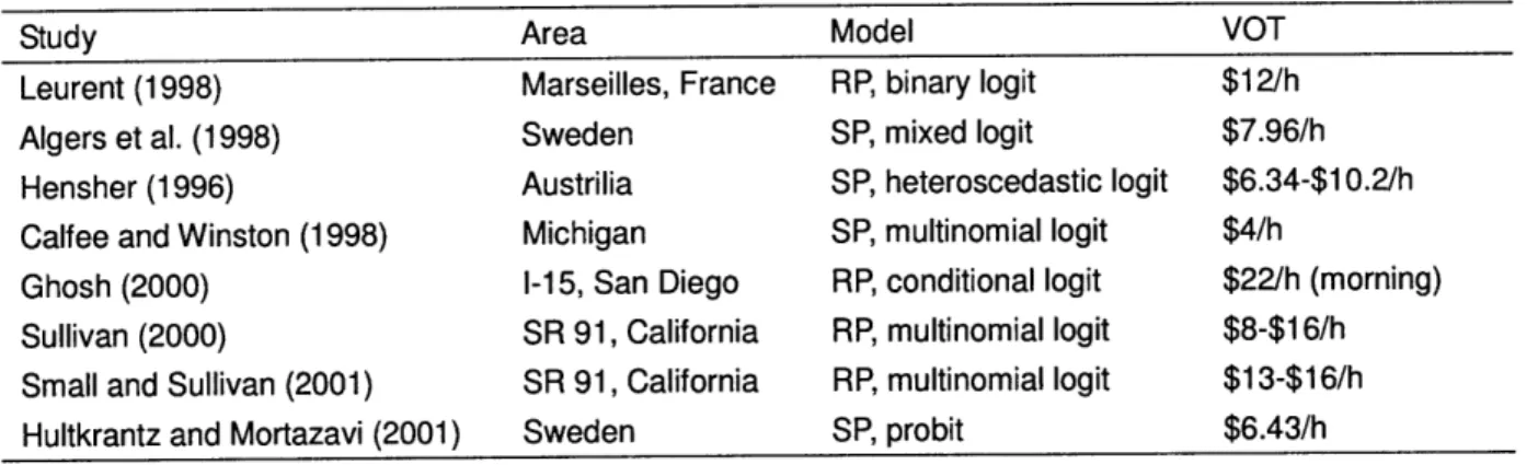
Table 3.1: VOT estimation based on discrete choice models ... 51
Table 3.2: Estimation of the early and late arrival penalty... ... 52
Table 4.1: Estimation results of SNOBFIT and SPSA ... ... 66
Table 5.1: 15-min flat toll scenario ... ... ... 85
Table 5.2: Optimal toll of SPSA for grad_rep=l (in cents) ... ... 92
Table 5.3: Optimal toll of SPSA for grad_rep=2 (in cents)...92
Table 5.4: Optimal toll of SPSA for grad_rep=3 (in cents)...92
Table 5.5: Best results for different grad_reps (in seconds) ... 92
Table 5.6: Optimal toll for FDSA-M (in cents)...97
Table 5.7: Overview of four toll strategies... 99
Table 5.8: Density difference between link 3 and link 4 (in vehicle/foot) ... 101
Table 6.1: Best toll strategy for LWC network (in cents).... ... ... 109
1. Introduction
Traffic congestion in urban transportation system is an increasing serious problem in major cities all over the world, causing tremendous economic and social problems, such as increased fiscal expenditure, air pollution, increased fuel consumption, and health related issues. Between 1980 and 1997, the aggregate US vehicle-miles traveled in urban transportation systems increased 67 percent, while the lane-miles only increased by 4 percent. As a result of the additional vehicle-mile traveled, the average annual hours of delay per vehicle increased from 100 percent to 300 percent (Skinner, 2000). Studies conducted in 437 US urban areas show that in the twelve months between 2004 and 2005, gas usage increased by 140 million gallons equaling about $5 billion, and aggregate travel time increased by 220 million hours. In 2005, estimated congestion costs amassed to approximately $78 billion as a result of wasted time and fuel (Schrank and Lomax, 2007).
Despite the worsening situation, there are ways to alleviate congestion from both the supply side and the demand side. From the supply point of view, congestion alleviation strategies are generally focused on building more facilities such as roads. However, urban road construction is very difficult and expensive.
From the demand point of view, congestion pricing is often considered one of the most efficient solutions for urban traffic congestion. In 1844, Jules Dupuit established the concept of "road pricing" by introducing a toll for the use of a certain bridge (Hager, 2004). Since the 20t century, it has been well established that people should be charged for road use (Knight, 1924; Pigou, 1912). While certain practical issues are still being discussed, congestion pricing is generally accepted as a good strategy for traffic alleviation and has already been applied or proposed in many cities around the world.
1.1 Overview of congestion pricing
Congestion pricing aims to relieve network congestion or to maximize revenue. While the latter is more often used by private road operators, the former is the focus of public concern. The aim of congestion pricing is to ensure a more rational use of road resources. This is accomplished by charging fees for the use of certain roads in order to reduce traffic demand or distribute traffic demand more evenly among the traffic network through the day. A toll is designed to relieve congestion by changing travelers' behavior. Different classes of users may respond differently to congestion pricing.
Congestion pricing is usually implemented in two main forms, pricing for roads or pricing for parking. Based on different toll strategies, road pricing is classified into three categories:
* Pricing at a cordon area: Drivers are charged a toll for road use in a specific area. The toll may be charged at the gantry when users enter the area or charged at a later time. The latter would require the use of electronic recording devices such as cameras to record and verify the presence of the user. This strategy is usually applied in metropolitan areas, and has been successfully implemented in Singapore and London.
* Pricing on urban roads: This strategy is popular in the US. The toll is collected manually or electronically for the use of a specific road. The tolls, which are collected on the road, may maintain a flat rate throughout the day, or vary based on the time of day.
* Pricing on single facilities: Drivers are charged for the use of specific transportation facilities. One example would be High Occupancy Toll (HOT) lanes where single drivers pay a fee for using HOT lanes, while drivers of high occupancy vehicles are exempted.
Road pricing is either link-based or path-based. Link-based tolls do not depend on a user's travel history because all users traveling through a certain link at the same time are charged the same fee. On the contrary, path-based tolls are dependent on the previous links of a trip. The tolls are based on a path rather than a link. Path-based tolls are difficult to implement in a real network because it is hard to specify each user's travel path. Therefore, for the purpose of
this thesis, only link-based tolls will be discussed.
Parking pricing is another component of congestion pricing that is aimed to control traffic by setting varying parking fees based on location, time, and traffic conditions. Parking pricing is considered an important part of congestion pricing and is applied almost all over the world.
Parking pricing is quite different from road pricing strategies in terms of principle and application. While road pricing is generally focused on relieving traffic congestion, parking pricing is usually implemented as a compensation for property maintenance, land use, and environmental pollution. Studies show that the elasticity of parking pricing is smaller than that of road pricing (Alberta and Mahalel, 2006). In addition, parking pricing may elicit diverse and unpredictable responses from users. For example, if a parking lot charges too much, a driver may continue to drive around in an attempt to find cheaper parking. This response to high parking fees may increase traffic congestion. The response to road pricing is often more homogenous and predictable, leading most researchers to recognize road pricing to be technically more efficient than parking pricing.
However, a stated preferences (SP) survey recently conducted as part of a parking pricing study shows that people tend to be more accepting of parking pricing than road pricing (Verhoef, 1995). People usually consider parking pricing as a regular fee for car ownership, similar to fuel tax and maintenance costs. In contrast, road pricing is regarded as a supplemental fee. Thus, from a political perspective, parking policies may receive broader acceptance.
Since this thesis focuses on the technical aspects of congestion pricing, the discussion will concentrate on road pricing. In the following chapters, unless otherwise specified, the term "congestion pricing" will refer to road pricing.
1.2 Response to congestion pricing
The use of congestion pricing to control network flow is based on the principle that travelers will respond to congestion pricing by changing route, switching departure time, changing travel mode, or canceling trip to avoid the toll. Responses to congestion pricing vary between individuals based on their socio-economic and demographic characteristics (income, gender, age, occupation, etc.). In addition, perceptions and attitudes of travelers also affect their decisions. Generally, responses to congestion pricing can be categorized as one of the five types listed in the following:
* Route choice: People may choose alternative routes to avoid a toll. Route choice depends on route attributes (e.g., toll, travel time) and the traveler's characteristics (e.g., familiarity with the network, value of time).
* Departure time choice: If the toll fluctuates throughout the day, travelers may change their departure time to avoid peak charges. Compared to route choice models, departure time choice models are usually much more complicated. Departure time models not only depend on the traveler's characteristics and travel times, but are also affected by penalties for early or late arrival which depend on factors like work schedule and flexibility. Departure time choice is a major focus in current congestion pricing research.
* Canceling trip: If the trip is unnecessary, the traveler may decide to cancel the trip in order to avoid the congestion toll.
* Mode choice: The traveler may also switch from private car use to other modes such as public transportation. Mode choice and the decision to cancel trips are sometimes considered together in congestion pricing research.
* Destination choice: For non-commuter trip travelers, they may change their destination to avoid the toll. This usually happens when people have many alternative destinations, and can choose one of them freely, e.g., shopping. There is no destination choice for commuter trips.
1.3 Static and dynamic congestion pricing
There are two strategies in congestion pricing: static congestion pricing and dynamic congestion pricing. In a static congestion pricing scheme, the toll typically stays the same, or varies but is predetermined for a long periods of time. The toll level is easy to determine and control which is why the static congestion pricing scheme is widely used in practice. Oslo in Norway is a good example of the static congestion pricing scheme. A recent research study indicated that after a static toll was introduced in Oslo, Norway, traffic was reduced by 5%
within the first year of operation (Ieromonachou, 2006).
In a dynamic congestion pricing scheme, the toll changes during the day based on traffic conditions on the tolled road. Although a pricing ceiling may established, travelers will not know the exact cost for their trips, but can only estimate based on the time of day, traffic conditions, and historical toll records. Dynamic congestion pricing schemes have demonstrated notable traffic alleviation in real world applications. In 2004, dynamic congestion pricing schemes were introduced in a traffic network in Santiago de Chile, at four different points in the network. The tolls were programmed to have three toll prices and to change from one pricing to the next based on the distance traveled, time of day, and speed of the traffic flow. Since 2004, drivers have reported a significant decrease in travel time. Road safety has also increased as a result of decreased accident rates (Road Charging Scheme, 2004). In Orange County, California, a variable toll that adjusts according to traffic flow and time of day was implemented on road SR 91 Express Lanes. Since the toll was implemented, the congestion on Highway 91 has dropped to a 15-year low (Yildirim, 2001).
A key concept behind congestion pricing is the economic principle that the toll should equal the marginal cost of the network users. Static congestion pricing schemes are unable to capture this principle, making it less effective than dynamic congestion pricing schemes which are able to capture this idea. Consequently, dynamic congestion pricing schemes have received much more attention from the research community.
For the most part, dynamic congestion pricing is still in the theoretical research stage. Although it has been applied in some cities such as Orange County in California (Yildirim, 2001), the toll prices are usually determined based on the traffic conditions of a single road instead of the entire network. There are various limitations associated with such an implementation. First, the network is an inter-connected system. The toll set on one link will affect the whole network. Therefore, to determine toll prices based only on a single road is unrealistic. Second, if the toll is only changed based on the tolled road, the traffic may alternate among several roads. This means that by relieving the congestion of one road, another road may become congested. Therefore, the current implementations of dynamic congestion pricing schemes are still immature.
1.4 Motivation
The dynamic congestion pricing models and algorithms are regarded as some of the most efficient ways to relieve traffic congestion, and are the subject of numerous research studies. However, past research studies have presented several drawbacks. First, some models only consider the route choice behavior, while some others only focus on the departure time choice. Although both aspects are significant, the combination of route choice and departure time choice is usually more important. Second, while most of the models have been tested using real case studies, they are based on network equilibrium rather than on users' choice behavior. Although the network equilibrium approach simplifies the simulation process, it does not adequately show the effects of congestion pricing on users' behavior. Third, almost all of the previous research efforts only tested models on small networks. To test the true validity and efficiency of the models, it is necessary to conduct a real case study using complex networks. These shortcomings motivate the need for further research in dynamic congestion pricing models.
DynaMIT, the software developed by the Intelligent Transportation System (ITS) lab at the Massachusetts Institute of Technology, provides a good resource for dynamic congestion
pricing research (Balakrishna and Sundaram, 2005). As a mesoscopic traffic simulation software, DynaMIT generates passenger simulations based on OD flow, people's characteristics, and the personal choice behavior of each user by using discrete choice models. DynaMIT then aggregates the passengers to calculate the final flow on each link. This process is repeated over time to simulate traffic on a specific network. In DynaMIT, each simulated user will be considered individually and his/her choice will be simulated based on current travel time and travel cost. Therefore, DynaMIT provides an excellent tool to test dynamic congestion pricing models based on users' personal choices.
Real data are also available. In collaboration with the New York State Department of Transportation (NYSDOT), real data can be obtained from the Lower Westchester County (LWC) network in New York State, including the network topology, OD flows and sensor data. The validity and efficiency of dynamic congestion pricing models can be analyzed and tested by performing a case study using the real LWC network.
This thesis focuses on dynamic congestion pricing modeling based on discrete choice models, and includes a case study that implements a newly developed dynamic congestion pricing model in the LWC network.
1.5 Implemented framework
The first task of this thesis is to develop a new dynamic congestion pricing model based on previous research. The model's objective is to find a toll strategy that minimizes the aggregate travel time of all network users. The following relationships are considered as constraints:
Network topology: paths, links and lane connections in the network; Supply parameters: the relationship between link travel time and link flow; Demand parameters: origin-destination (OD) flows;
discrete choice framework.
An experiment to examine the model on a test network will be required. In order to consider users' personal choice, this model will be implemented in DynaMIT. The chosen test network for this experiment has been used for testing in DynaMIT for several years. Some parameters will be calibrated, while others may be cited from other studies.
A real case study will be conducted using the LWC network in New York State. With hundreds of links and nodes, this network is complicated enough for model testing. In addition, the LWC network has been featured in previous research (Vaze, 2007; Rathi, 2007). The calibration and simulation results from previous research studies can be cited and compared to the current congestion pricing research.
1.6 Contribution
This thesis focuses on the development and testing of the dynamic congestion pricing model. Compared with previous studies, this model has several advantages.
First, the model is based on travelers' choice behavior. Compared with the deterministic network equilibrium approach used in previous models, this method with stochastic behavior choice can explain travelers' uncertainty of response to congestion pricing more realistically.
Second, by considering route choice and departure time choice together, the model is able to provide a more comprehensive view of the different effects of congestion pricing, making the results more credible and persuasive.
Third, after initial examination on a test network, the model is tested in a case study on the LWC network. The case study provides a more reliable estimation of the validity and efficiency of the model as well as dynamic congestion pricing.
1.7 Outline
This thesis is organized as follows. Chapter 2 provides a literature review on models, algorithms and tests on congestion pricing, especially for dynamic congestion pricing. Chapter 3 presents a newly developed model that incorporates users' choice behavior using a discrete choice framework. The route choice and departure time choice are presented in this regard. Chapter 4 discusses the methods and algorithms to solve the model presented in Chapter 3. Chapter 5 presents the evaluation of different algorithms based on the experiments
conducted using a test network. A modified version of Finite Difference Stochastic Approximation (FDSA) algorithm (FDSA-M) is selected as the best method. Chapter 6 presents a case study where the model from Chapter 3 is analyzed and tested on the LWC network in New York State. Finally, the research conclusions are provided in Chapter 7.
2. Literature Review on Dynamic Congestion Pricing
Congestion pricing has been studied worldwide for several decades. Previous congestion pricing studies usually concentrated on the static aspect, in which the congestion tolls were either flat or pre-set along the day. Although static congestion pricing neglects several significant issues, the models and results in route choice and departure time choice are still quite valuable to be applied in the dynamic congestion pricing model. Recently, dynamic congestion pricing receives more attention than before. Newer models for both analysis and simulation have been developed.
The literature review is structured in the following manner: First, the materials on route choice model and departure time choice model are summarized and analyzed. Next, the studies on the general structure of congestion pricing, especially dynamic congestion pricing, are discussed.
2.1 Route choice models
Route choice is crucial for dynamic congestion pricing. Every commuter trip faces route choice. Although travelers usually have a habitual route for a commuter trip, they may switch to another path to avoid congestion or a toll. Thus, route choice should be considered
significantly in every congestion pricing model.
In route choice models, one of the most important issues is how to simulate the uncertainty of travelers' choices. Two main methods are discussed in this regard, fuzzy logic and discrete choice model. The potential application of previous research in this thesis is also discussed.
2.1.1 Fuzzy logic
Fuzzy logic is derived from fuzzy set theory which deals with reasoning by approximation rather than precision. Fuzzy logic allows the user to set values ranging between 0 and 1. Its linguistic form expresses the concepts similar to "slightly", "quite" and "very", known as degrees of the truth, which denotes the extent to which a proposition is true. Degree of truth should not be confused with a probability. For a detailed introduction of fuzzy set and fuzzy logic, see Zadeh (1965).
Fuzzy logic is shown to be a very promising mathematical approach to modeling traffic and transportation processes. It has been applied in various traffic and transportation problems, especially in route choice (Teodorovic and Kikuchi, 1990; Akiyama and Yamanishi, 1993; Lotan and Koutsopoulos, 1993; Akiyama and Tsuboi, 1996). Teodorovic (1999) has provided a good summary on the fuzzy logic research in route choice modeling.
The first application of fuzzy logic in route choice can be found in Teodorovic and Kikuchi (1990). In the paper, an algorithm based on fuzzy logic is developed to solve a two route problem. In this example, route choice simply depends on the travel time. Denote the travel time on route A and B as TA and TB; the fuzzy sets of TA are thus represented as: MLTB
-much less than TB; LTB - less than TB; GTB - greater than TB; and MGTB - much greater
than TB.
Two fuzzy indices PA and PB are used to represent users' preferences for the respective routes. Thus, they are two positive values that sum up to 1. PA and PB are highly correlated to the fuzzy sets. For example, if TA = MLTB, PA is a large number; whereas if TA = MGTB, it is very small. The exact value of PA can be calculated based on the travel time relationship between the two routes.
When multiple travelers are generated on the network, an algorithm is developed to determine the number of users in each route based on the previous discussion. The users are generated
randomly depending on the network characteristics, e.g., the distribution of travel time. The number of users is simply obtained by adding all PA and PB up.
This algorithm, although simple, provides a general structure of fuzzy logic application in route choice model.
Akiyama and Yamanishi (1993) have developed another structure of route choice model using fuzzy logic. The authors first conduct a survey to determine the allowable ranges between the informed travel time and real driving time; a triangular fuzzy number (TFN) structure is obtained from the results of the survey. The authors then improve the TFN structure by three methods. The first method (Method I) is generally used to express the similarity which is related to fuzzy truth values. The second method (Method II) can be explained by equality relation between usual numbers with the extension principle. And the third method (Method III) considers the distributed area of TFN.
A test is then conducted to examine the three methods. Method III is found to provide the largest informed travel time, followed by Method II and Method I. Although their results are not as stable as Method I, Methods II and III are still recommended as better approaches after a comparison of their advantages and disadvantages.
Fuzzy logic has been successfully used in traveler's route choice model. However, there are several limitations that confine the further implementations. First, it is lack of theoretical basis to simulate traveler's behavior choice by fuzzy logic. Although the simulation results seem reasonable in many case studies, it is hard to explain traveler's behavior choice from the results. Second, there is still no implementation of fuzzy logic in complex networks. Without the test in real network, the usefulness and effectiveness of fuzzy logic model in route choice area is in doubt.
2.1.2 Discrete choice model
Discrete choice models deal with the problems that involve choices among two or more discrete alternatives. The theory of discrete choice is now well developed and the application is widespread in numerous areas, such as, marketing, shopping and transportation.
In transportation, discrete choice models have been successfully applied to mode choice, traffic assignment, airline management, etc. For detailed descriptions about the theory of discrete choice model and its application, see Ben-Akiva and Lerman (1985).
Discrete choice model has been successfully used in route choice by many researchers. Ramming (2002) has shown the advantages to apply discrete choice model in route choice. These advantages include, excellent simulation results, the ability to explain traveler's behavior and easy to implement.
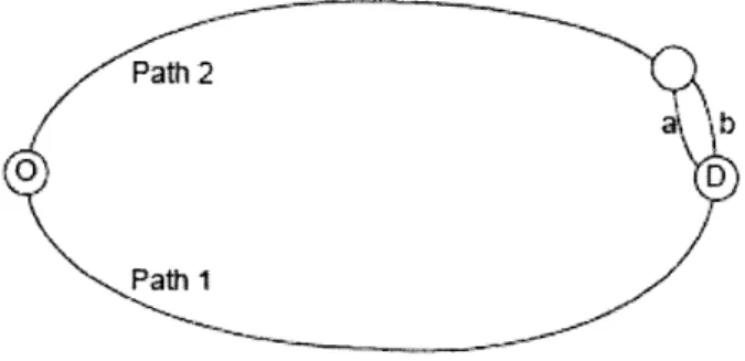
Ben-Akiva and Lerman (1985) describe a famous example which is often cited by other researchers. This example is usually used to prove the powerfulness of nested logit (NL) model over simple multinomial (MNL) logit in specific problems, including route choice. In this example, two paths are under consideration as shown in Figure 2.1. Near the destination path 2 gets divided into two sections.
Path2 2"
P-1
Figure 2.1: Path choice problem
Only consider travel time in the utility function, and assume the travel time in the two paths are the same. Thus, without considering a and b, the system part of the utility for path 1 and
path 2 are exactly the same, leading to the probability for choosing each of them to be 50%.
Now consider the small sections a and b as well. There are three paths in the network now: path 1, path 2a and path 2b. Based on the multinomial logit (MNL) model theory, since the travel time among the three paths are the same, the probability to choose each of them is 1/3.
However, this result is unreasonable, because most users cannot identify the difference between path 2a and path 2b, and the probability to choose path 1 and 2 is therefore the same as the previous example, which is 1/2.
The reason for this paradox is that the independent and identically distribution (i.i.d.) property does not hold for path 2a and path 2b, since they overlap each other for most of the part. The paradox can be solved by using a nested logit (NL) model in which the correlation between E2a and 2b is considered by a nested structure, where path 2a and path 2b are in the same
branch, and path 1 is in another separate branch. The result of the nested logit model is correct.
Although NL model is more powerful than MNL model in route choice, there are still several problems. The most serious problem is, the overlap among different paths is hard to consider in practice. In the previous example, one can simply conclude that the overlap of path 2a and path 2b is very high, so that the nest can be built by assigning them to the same branch. But in the real world, if the overlap of two paths is not so high, it is hard to decide how to build the nest structure. In order to improve it, several other models are developed.
Koppelman and Wen (2000) have developed a paired combinatorial logit (PCL) structure for the route choice problem. In the NL model, covariances are assumed to be equal among all alternatives in a common nest, and zero otherwise. PCL model relaxes the restrictions by allowing for different covariances for each pair of alternatives. The advantages of PCL model are that different competitive relationships can be estimated between each pair of alternatives; and the closed form of the PCL model is computationally less intensive when compared to
other logit models.
The PCL model is a member of the generalized extreme value (GEV) family of models (McFadden, 1978). PCL and NL are both general cases of the MNL model; but none of them is a restricted case of the other. In route choice, PCL model can deal with the problems that can not be formulated by NL model. For example, a three path cases in which path 2 is overlapping with path 1 in one section, and is overlapping with path 3 in another section.
Cascetta (1996) has developed a structure for considering the overlapping of the routes, known as C-logit model, which is a modified MNL model. Although some overlapping can be explained by NL and PCL model, when network expands, the nested structure is very hard to build. C-logit uses a different modification from the MNL model by introducing a term called "commonality factor", which can be interpreted as the degree of overlapping of one path with other paths. The commonality factor is added in the utility function of a path to decrease its utility based on the level of overlapping.
A case study was performed based on a sample of 1471 paths chosen from truck drivers on the Italian inter-city road network. The results show significant improvements by the C-logit
model to the MNL model specification.
Bekhor et al. (2002) have developed another structure to incorporate behavioral theory in the C-logit adjustment process, known as Path-Size logit. Path-Size logit adds a "size" variable the utility of alternative routes:
exp (Vi, + In Si,) (2.1)
P(i I C,,)= (2.1)
Yexp
p(V±,, + In Sj,)je C,
where C, is the available path set for traveler n; V,, and Vj, are the utilities for the path i andj for traveler n, respectively; t represents a scale parameter; and S,, and Sj,, are the size variables for path i andj for user n, respectively. The size S,, is defined by:
Si=
l
j1 (2.2)Z aj L. jeG, Lj
where iT is the set of links in path i; la and Li are the length of link a and path i, respectively;
6aj is the link-path incidence variable that is one if link a is on path j and 0 otherwise; and
L: is the length of the shortest path in C,.
Ramming (2002) has performed a comparison among many different models in route choice including MNL, NL, C-logit and Path-Size logit, and recommended Path-Size logit as the best. In his thesis, Ramming (2002) also performed a lot of experiments to demonstrate the usefulness and effectiveness of discrete choice model.
Unlike fuzzy logit, discrete choice model has a solid theory base, and can explain the personal behavior choice clearly. Based on all these advantages, it is selected as the model used in this thesis.
2.2
Departure time choice models
Departure time choice is another important part in congestion pricing model. In response to congestion tolls, users may change their departure time similar to changing a route on the network. Departure time choice is more complex than route choice, because while users can choose their routes freely, they cannot depart at any time they want. There is an additional penalty for deviating from the habitual departure time. On one hand, people should arrive on time for commuter trips, so they cannot delay their departure too much; whereas on the other hand, most people do not want to depart too early in the morning either. Thus, the penalty for
Departure time choice has been attracting a lot of attention recently in research. Various structures have been developed to formulate it. However, none of them are well accepted.
In a recent paper, Borjesson (2008) developed a mixed logit model to analyze departure time choice. In trip timing modeling, scheduling disutility is formulated as a function of departure time shifts from the most preferred departure time (PDT). The shifts are defined as schedule delay early (SDE) and schedule delay late (SDL):
SDE, = max[PDT7 - D,, 0] (2.3)
SDLin = max[DTin - PDTn, 0] (2.4)
where DT is the departure time, i refers to alternative and n represents different individuals.
The author considers three alternatives for stated preferences (SP) data, two for cars and one for public transport. The utility functions are defined as a combination of travel time, travel cost, SDE, SDL, and the variability of travel time. While combining with the revealed preferences (RP) data, cost is not available. Thus, cost is not considered for the RP data.
For each individual, consider a SP alternatives sequence isp = i,...,iK} , and a RP
alternative iRP, = {K+1 }. Assuming that the random parameters are independent between RP and SP choices, the conditional probabilities for each sequence can thus be presented as a logit function. Then the unconditional probabilities can be simply calculated by an integral of the conditional probabilities.
The model is then tested by RP-SP data. The reliability ratio is estimated to be 0.74, which is inline with an earlier study (Black and Towriss, 1993). However, this paper does not provide a comparison between the results with other methods. Therefore, the efficiency of the model is in doubt.
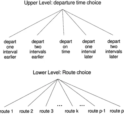
Antoniou (1997) has developed the departure time choice structure based on discrete choice model. In his master thesis, Antoniou introduces a general structure of the demand simulation tools for Dynamic Traffic Assignment (DTA), in which the departure time choice is determined within a more general trip decision structure. A time discretization is applied in the departure time choice model, in which the departure time is split into five intervals: depart two intervals earlier; depart one interval earlier; depart on time; depart one interval later; depart two intervals later. In this structure, interval length is critical, and is pre-set by experience and experiments. The five-interval structure can be expanded to more time intervals.
In this structure, departure time is considered together with route choice, where a combination of one departure time and one route is considered as one alternative. A MNL model is applied to determine the right departure time and route. In this process, some weighting are applied in each time interval to capture the passengers' willingness to change departure time, as well as the penalty for early and late arrivals. Weighting parameters are determined by calibration.
Ozbay and Tuzel (2008) have used another approach to consider the departure time choice. In their paper, the authors develop a mathematical formulation at the beginning, in which maximum available early arrival and maximum available late arrival are considered. By applying the Lagrangian multipliers, several important values are obtained, including marginal utility of additional income and marginal utility of additional available time. The authors then analyze the mathematical formulation stepwise to get a utility function, in which the utility is formulated by a complex relationship of travel time, travel cost, deviation from desired arrival time, the time difference between departure and desired arrival time.
The authors then apply this utility in a NL model in a case study in New Jersey Turnpike (NJTPK) to calculate the value of time (VOT) on it. The mean and standard deviation for VOT range from $15/h to $20/h and $2/h to $3/h, respectively, which are consistent with previous research.
Jou et al. (2008) have developed a departure time choice model for commuter trip in the morning. In this model, five different time variables are used: departure time, earliest acceptable arrival time, preferred arrival time, actual arrival time and work starting time. Based on the five times, the time line is divided into four sections, known as early-side loss (segment I), early-side gain (segment II), late-side gain (segment III) and late-side loss (segment IV). The utility of these four sections are all composed of a deterministic part and a random section.
Assuming the random errors are normally distributed, the authors calculate the probability of each segment. The model is then solved by maximum likelihood method. All of the estimators
can be estimated accordingly.
The model is tested by a survey data conducted in Taiwan in 2002. It is found that most (52%) of the arrivals are within 5 minutes of their preferred arrival time, and 75% are within 10 minutes. The gain and loss of a late-side are observed to be greater than those of early-side, which is consistent with previous research.
Departure time choice is still an immature area, in which none of the model is well accepted. Among all these models, Antoniou's model based on discrete choice structure is suitable for the dynamic congestion pricing model in this thesis, and is proved to be useful in several real time case studies (Vaze, 2007; Rathi, 2007). Although some modifications are necessary, this model provides us a good approach to consider the departure time choice in congestion pricing model.
2.3 General congestion pricing models
In this section, some general congestion pricing structures are discussed. While the paper in previous sections usually focus on one aspect of congestion pricing, the models in this section
all concentrate on the whole picture of congestion pricing. Generally, these methods and algorithms are classified in two types: analysis model and simulation model.
2.3.1 Analysis model
In analysis model, the research usually concentrates on the correctness and completeness of the model, rather than its application. The model is usually quite complex, and requires complete information about the network and users. While providing some theoretical perspectives, the model cannot be applied in practice.
Wie and Tobin (1998) is a good example of analysis model. In the paper, the authors develop two types of dynamic congestion pricing model based on the marginal cost pricing theory. In the first model, the arc capacities and travel demands are stable from day to day; while in the second model, both of the capacity and travel demands fluctuate significantly. The authors show that two type questions can both be solved by a convex control formulation of the dynamic system optimal traffic assignment problem with several different origins and destinations. The equilibrium of the models is proven at last.
In this paper, a general structure of dynamic congestion pricing is developed and proven. One can examine several significant conclusions theoretically by the model. However, in the application part, there are still many works left. First, the homogeneous user assumption is irrational. The authors fail to consider any users' behavior, e.g., route choice and departure time choice in their model. Second, it is almost impossible to charge different users different tolls at the same link based on their destination. Generally, a standardized toll will be charged for all the users (or based on users' type, e.g., cars and trucks) on a link.
In addition, in almost all analysis models, too much information is required to determine the optimal toll. It is too difficult to implement them in practice. This is a common limitation of all analysis models. This limitation confines the further development of analysis models.
2.3.2 Simulation model
In simulation model, researchers focus on the application of the algorithm. The model is usually less complex but more applicable than analysis model. In addition, the authors often provide an example to test the algorithm. Although simple, the example explains some characteristics of congestion pricing. Because the purpose of congestion pricing lies upon its application, the simulation model is regarded as the focus of the congestion pricing research, e.g., Yan and Lam (1996), Verhoef et al. (1996), Joksimovic et al. (2005) and Verhoef (2002).
Verhoef et al. (1996) have used a two-link network simulation model to examine the effects of various demands and cost parameters. Several important topics are discussed and tested in the simple network. Some basic welfare economic properties are discussed for the network with one route tolled and the other untolled. The factors determining the relative performance of one-route tolling are examined. It is found that the lower the two cost parameters (one for free-flow cost and the other for congestion cost) on the tolled route, the more attractive the tolled route becomes. With identical routes, the attractiveness of the tolled route increases with the elasticity of the demand. It is also found that with fixed cost or regulation, the strategy of tolling one route is more efficient than tolling both routes, especially if the cost parameters for the untolled route exceed that for tolled one. The paper also examines the toll strategy by maximizing revenue. This paper, while too simple by considering only a two-route network, provides several useful concepts for congestion pricing.
Yan and Lam (1996) have developed a bi-level structure for determining the optimal toll. A bi-level programming problem has been applied in traffic assignment successfully before (Yang and Yagar, 1994; Yang, 1995). The authors introduce this method into this paper to solve the optimal toll problem. Although the authors only consider the static congestion pricing based on route choice, this bi-level structure is applied broadly in the future dynamic congestion pricing research.
The general structure of a bi-level programming is:
min F(u, v(u)) (2.5)
s.t. G(u,v(u)) 0 (2.6)
where v(u) is implicitly defined by
min f (u, v) (2.7)
s.t. g(u,v) 0 (2.8)
where F is the objective function of upper-level decision maker (in this case, system manager);
u is the decision vector of upper-level decision maker (in this case, road toll); G is constraint
set of upper-level decision vector;f is the objective function of lower-level decision maker (in this case, network users); v is the decision vector of lower level decision maker (in this case, network flow); and g is a constraint set of lower-level decision vector.
In the bi-level structure, the system manager chooses toll values u to optimize his objective function F. The network users, after obtaining the information about the system manager's decision, make route choice to minimize their travel cost. The network flow v(u) is thus determined by aggregating their decisions. Moreover, for any given toll pattern u, it is assumed that there is a unique flow distribution v(u), which is obtained from network equilibrium at the lower-level problem. v(u) is also called the response or reaction function. The optimal toll level u greatly depends on the evaluation of the reaction function v(u). In other words, users' route decision corresponds to toll charges.
The algorithm is performed by iteration. First, an initial toll pattern u is selected. Second, the network flow v(u) is calculated by network equilibrium in the lower-level problem. Third, the
upper-level objective function is formulated by a local approximation, and a new toll is determined by solving the approximation problem. If the new toll is close to the original one,
stop; otherwise, go back to the lower-level again.
The authors then develop two algorithms based on this general structure, applying different optimization method and different strategies to determine the new toll. Two examples are used to test the algorithms. While the examples are quite simple, the results reveal some interesting properties of congestion pricing, and demonstrate the efficiency of the algorithms.
Verhoef (2002) has described an algorithm to calculate the second-best optimal toll levels and toll points in general networks, and test the algorithm in a ten-link network. The algorithm in this paper, although only based on a static research, expands the scope of congestion pricing model, because it can be used for studies of various archetype pricing schemes, including cordon toll, single major highway pricing and parking policies.
The author first develops a model for the fixed location toll. The algorithm determines network equilibrium based on the economic equilibrium principle in which marginal benefits equal marginal private costs, which is known as the standard Wardrop condition (Wardrop, 1952). The optimal toll level is determined by maximizing social welfare, which is defined as total benefits minus total costs. The algorithm is therefore described as two steps. First, for a given network equilibrium with user level, compute the solution to the optimization problem. Second, implement the tolls in the network to get new network equilibrium. The two steps are repeated until convergence.
A numerical example in which some other toll strategies are also implemented in the model is conducted as follows. The network has ten links, three origins and two "real" destinations (W and Y&Z). Since the second destination has different parking strategies, it splits into two different parking nodes, Y for private parking and Z for public parking. Two virtual links are added connecting to Y and Z. In addition, a link with lane charge restriction also splits into two parallel links, one free and the other tolled. The test shows that most of the toll levels
converge for an accuracy limit of 1% by five iterations or less. However, an exception exists, for that lane the toll converges for no less than 250 iterations.
The author examines the toll points in the next part. The first single toll point is determined by an indicator Ix, which predicts the welfare gain from implementing a toll on link x from no-toll equilibrium. The algorithm performs very well in the first toll point searching, in which the correction between true and predicted welfare gains is 0.9987. In multiple toll-points case, three attempts have been tried: selecting the toll-points based on the several highest scores; selecting toll-points one-by-one, taking previous toll points given; or, selecting the set of toll-points simultaneously. Among them, strategy two is observed as the best one by considering the accuracy and computation load together. Some combination methods of the three algorithms are also discussed without simulation test.
This paper provides several new ideas, e.g., parking pricing implementation and toll-points determination. However, the author only considers network equilibrium to calculate the network flow. Users' behavior is excluded, and thus cannot be reflected by the model.
Joksimovic et al. (2005) have designed an optimization structure based on the bi-level programming by Yan and Lam (1996). On the upper level, a Mathematical Problem with Equilibrium Constraints (MPEC) formulation is applied to determine the optimal toll by considering the dynamic nature of traffic flows; on the lower level, users' behavior will be considered in route choice and departure time choice by discrete choice model.
The model is composed of three major sections, that is, dynamic network loading (DNL), users' behavior and the road-pricing model. While the road-pricing model is on the upper level, dynamic network loading and users' behavior model constitute the lower level, known as dynamic traffic assignment (DTA) model, which can be converted into an equivalent variational inequality (VI) problem. We describe the two parts of the model separately.
focus of this part. In this part, users' behavior is characterized by a combination of route choice and departure time choice. An appropriate random utility discrete choice model will be used for this purpose. In the users' utility function, both dynamic travel time element and dynamic road-pricing toll element are contained. The departure time choice is considered by introducing penalties for deviating from the preferred arrival time (PAT) and preferred departure time (PDT), a similar approach using in several research (De Palma and Rochat, 1995; De Palma and Fontan, 2001; Gabuthy et al., 2006).
Based on the calculation of the lower level, the road pricing model can be expressed as an optimization problem in the upper level. Mathematical problem with equilibrium constraints (MPEC) is a special case of a bi-level structure where the upper level is an optimization problem and the lower level is an equilibrium problem, refer to Luo et al. (1996) and Lawphongpanich and Hearn (2004).
The bi-level problem is solved iteratively until it converges or reaches certain loops. During the process, the tolls are updated by a simple grid-search procedure each iteration. Some experiments are performed on a simple network that comprises three links.
This paper leads to a good approach to consider the dynamic congestion pricing. The bi-level structure is improved in this paper, where discrete choice model is implemented in the lower level to formulate users' behavior in both route choice and departure time choice, and an optimization problem is developed in the upper level to determine the optimal toll.
This model presents a complete structure of congestion pricing model, in which both route choice and departure time choice are considered. However, there are still some problems in the structure. First, the model considers network equilibrium instead of travelers' behavior choice; second, the optimization algorithm in this paper, a simple random search, is not efficient for big networks; last but not least, just as all previous research, no real case study is performed.
Simulation model has several advantages: first, although simplifying a lot, many models still have good theoretical basis; second, the models are usually easy to apply in the real network, and a case study, although simply, is usually followed after the theoretical discussion; third, the simulation model is easy to absorb good results from other research, e.g., early and late penalty for departure time choice. Therefore, simulation model attracts more attention in the dynamic congestion pricing model research.
Nevertheless, several limitations still exist in simulation model. First, the model always uses deterministic network equilibrium, rather than users' stochastic choices, to determine the network flow. Second, the optimization algorithms are usually inefficient. An appropriate optimization method should be suggested. Third, the test network is too small to examine the validity and efficiency of the algorithms. A real case study is necessary to test the model and algorithm, but is rare in the congestion pricing research today.
2.4 Summary
Current dynamic congestion pricing research is classified into two types: first, focus on the users' behavioral responses to congestion pricing; second, develop general frameworks of congestion pricing model.
Within the users' behavior model research, route choice model and departure time choice model attract the most attention. Two methods are summarized in the route choice model: fuzzy logic and discrete choice model. While fuzzy logic is successfully used in some research, the uncertainty of users' behavior in route choice is explained better by discrete choice model. Departure time choice is more complex than route choice. Penalty is difficult to formulate. Various studies are conducted in this topic, but none of them are well accepted.
Research concentrated on general structure of dynamic congestion pricing often focuses on two aspects of this topic: analysis model or simulation model. Although the analysis model
sheds light on some theoretical viewpoints, it is difficult to implement in the real network. Therefore, the simulation model attracts more attention. The effect of dynamic congestion pricing is observed in a lot of research. However, current research on the simulation model has several drawbacks. First, the network flow is determined by network equilibrium rather than users' choice behaviors in most research. Without users' choice behavior, the characteristics of behavior response cannot be reflected in deep. Second, most studies only focus on some aspects of the behavior model. The full set of the behavior model, i.e., route choice, departure time choice, mode choice and canceling trip choice, is rarely considered. Third, the test is only performed in a small network in all the research. However, a case study in real network is necessary to examine the validity and efficiency of dynamic congestion pricing.
3. Model Development
In the previous chapters, the existing literature on dynamic congestion pricing has been summarized, and the common limitations in previous works have been highlighted. The major limitations include ignoring travelers' personal choices in the simulation process, failing to choose efficient optimization algorithms, and the lack of case studies on large networks. In this thesis, these limitations will be addressed by a new model. In this chapter, a new dynamic congestion pricing model based on a discrete choice framework is presented. Instead of considering network equilibrium, this model simulates travelers' choice behaviors on their routes and departure time. The structure of the model is implemented in DynaMIT, a
mesoscopic transportation simulation software developed by MIT ITS lab. In Chapter 4, optimization algorithms to operationalize the model are discussed and summarized. Based on previous research, appropriate algorithms are selected and tested on a small network in Chapter 5. A real case study is performed on a network from New York state in Chapter 6.
This chapter is organized as follows: first, the mathematical formulation of the proposed model is developed; second, the values of the important parameters in the model are estimated
and calculated.
3.1 Mathematical formulation
In congestion pricing problems, the mathematical formulation is critical. It not only provides a good tool for theoretical analysis, but also presents a clear explanation for the basic concepts of the problem.
problem, where the objective is to minimize the total travel time of all passengers in the network, and the constraints are governed by the network topology, demand, supply and choice behavior of the travelers. All these concepts are discussed in detail below. The
simulation conducted in the following chapters is based on this formulation.
3.1.1 Optimization formulation structure
Depending on different purposes, the objectives of congestion pricing can be separated into network optimization and revenue maximization. While the latter is sometimes used in some private companies, the former is the focus of congestion pricing research. Several different quantities can be used to measure the network condition, e.g., total travel time, social welfare and consumer surplus. While the latter two are feasible for both elastic and inelastic demand, the total travel time is only feasible for inelastic demand. But compared to the social welfare and consumer surplus, the total travel time is the more intuitive reflection of the effect of congestion pricing. Since only route choice and departure time choice are considered in this thesis, the demand can be assumed to be inelastic, and the objective function is chosen to minimize the total travel time among all travelers. The optimization problem can therefore be written as:
Min T(x,S,),, ,e)
(3.1)
x S. t.f (x, S, D,
A,e)
=0
(3.2)
Ix <X x ux (3.3)where T is the total travel time experienced by all drivers, x denotes the costs (tolls) to be optimized, and S, AD, AV and C represent supply parameters, demand parameters, network
topology and travelers' choices, respectively. x are the only unknown parameters in this optimization problem, and are bounded from below by lx and from above by ux.