DESIGNING AERO-ACOUSTIC WALL OPENINGS FOR NATURAL VENTILATION
by
Sephir D. Hamilton
B.S., Mechanical Engineering (1999) Clarkson University
Submitted to the Department of Mechanical Engineering in partial fulfillment of the requirements for the degree of
MASTER OF SCIENCE IN MECHANICAL ENGINEERING at the
MASSACHUSETTS INSTITUTE OF TECHNOLOGY June 2001
@ 2001 Massachusetts Institute of Technology All rights reserved
MASSACHUSETTS INSTITUTE OF TECHNOLOGY
LIBRARIES
Signature of Author ..
Department of Mechanical Engineering May 11, 2001
Certified by ...
A 1v d b ~~...
Leon Glicksman Professor of Mechanical Engineering Thesis Supervisor
..
.-.. .. . . .Ain A. Sonin roI eJ y. ....... ..
DESIGNING AERO-ACOUSTIC WALL OPENINGS FOR NATURAL VENTILATION
by
SEPHIR D. HAMILTON
Submitted to the Department of Mechanical Engineering on May 11, 2001 in partial fulfillment of the requirements for the degree of
Master of Science in Mechanical Engineering.
ABSTRACT
Building designers and owners continue to avoid natural ventilation despite the promise of significant annual energy savings. The fact is, natural ventilation is riddled with problems.
Acoustic privacy, air quality, humidity, and fire safety are just four problems associated with
natural ventilation that place it far short of meeting current living standards in many countries.
This thesis focuses on overcoming the problem of noise privacy by proposing new designs, dubbed
"aero-acoustic wall openings," that permit natural ventilation without sacrificing acoustic privacy. Instead of opening doors and windows, people will open these aero-acoustic wall openings to let in air for natural ventilation.
Two aero-acoustic wall opening designs (a transfer duct and a U-shaped duct) are investigated and refined to meet design goals for noise transmission loss and pressure loss. Empirical and
theoretical models predict the performance of the designs, and experiments verify the predictions.
The final V-shaped duq design has a sound transmission class (STC) rating of 25 (comparable to
well-sealed doors and windows), and allows 10 air changes per hour (ACH) through three walls (in series) of a standard 120m2 (1614ft2) apartment under a total pressure gradient of 8Pa (produced by wind
speeds of 3.7mI/s - 8.3mph), while occupying only 20% of the available wall area. Profit margin
estimates are promising (50% - 83%) and encourage bringing aero-acoustic wall openings to market. Whether for an office building, a private home, or a large apartment complex, aero-acoustic wall
openings are easily integrated with the architecture to produce an aesthetically pleasing and energy-efficient building. Hopefully, now with one less reason to avoid it, and every reason to use it, building designers and owners will freely adopt natural ventilation for buildings.
Thesis Supervisor: Leon Glicksman
Table of Contents Title Page ... 1 Abstract ... ---... 2 Table of Contents ... 3 Acknowledgments ... 5 Chapter 1 - Introduction...7 1.1 Purpose 1.2 Background 1.3 Natural Ventilation Basics 1.4 Acoustics Basics 1.5 Existing Technology 1.6 Possibilities 1.7 Overview Chapter 2 - Prototype Design ... 19
2.1 Reference Case 2.2 Design Goals 2.3 Existing Technology - Performance 2.4 Design Ideas 2.5 Acoustic Prediction 2.6 Airflow Prediction 2.7 Initial Prototypes Chapter 3 - Experiments ... 37 3.1 Acoustic Experiments 3.1.1 Procedure 3.1.2 Results 3.1.3 Discussion 3.2 Airflow Computation (CFD) 3.2.1 Procedure 3.2.2 Results 3.2.3 Discussion Chapter 4 - Refined Designs ... 57
5.2.1 Cost
5.2.2 Performance
5.2.3 Life Cycle Analysis 5.3 Future Exploration
Chapter 6- Conclusion... 72 6.1 Summary
6.2 Vision of the Future
References ... 74 Appendix A. Experimental Data ... 76 A. 1 Receiver Room Absorption Test Data
A.2 Transmission Loss Test Data for Straight Ducts A.3 Transmission Loss Test Data for Prototypes A.4 Output from CFD Computations
Appendix B. Supporting Material ... 91 B.1 Kammerud, et. al. (1984) Study on Ventilation Energy Savings
Acknowledgments
This thesis work was sponsored by the Kann-Rasmussen Foundation and the Alliance for Global Sustainability. Carl Rosenberg of Acentech Corporation helped get the work off the ground with advice and guidance on acoustics. John Doherty's generous assistance and expertise was
instrumental in the success of the acoustic experiments, and BBN Technologies graciously provided the experimental facilities. Professor Leon Glicksman allowed me to explore the horizon, then skillfully guided me back to earth during the two years I was fortunate enough to have him as my thesis advisor and personal mentor.
Patricia Alikakos gave me comfort, support, and encouragement when I needed it most. I will be forever grateful for her patience and for our lasting friendship.
Chapter ]
Introduction
1.1 PURPOSE
The year is 1953. The first color televisions are sprouting up in homes across the United States, and one of those marvelous Carrier air-conditioning systems was just installed at the new movie theater across town.
It's early evening now; all the windows of your ranch house are open
-and maybe even the front door - when a merciful splash of cool air forges a path through the hallway, past the kitchen, and into the living room where it laps at the sweat beading-up on your forehead. How pleasant the chilling breeze feels on your body after a long, hot, sweat-filled day at the factory.
Later, as you drift into sleep under a thin cotton sheet ever-so gently touched by the cool breeze, the neighbor's cat screams out a moan that rattles even the retinas in your eyes. You jolt to the open window next to your bed and slam it down; anything to silence these haunting screams of feline passion. This act, however, proves a fatal mistake as you lay back in bed and realize that even without the cotton sheet over your body, your skin is drowning in a sticky layer of sweat now that you've locked the breeze outside. If only you could install one of those new Carrier air-conditioner systems right in your home like they do at the movie theater, so you could close the window and still be comfortable.
The evolution of mechanical air-conditioning systems over the last century (the Carrier Corporation was founded in 1915) has helped people realize the dream of having thermal comfort without sacrificing acoustic privacy. In fact, building occupants today expect and demand acoustic privacy along with thermal comfort. Air-conditioning, however, is only one solution for ensuring thermal comfort and acoustic privacy in buildings. For the sake of energy conservation, a better solution would utilize natural ventilation and solve the noise privacy problems associated with it. That "better" solution is the goal of this thesis.
1.2 BACKGROUND
This work evolved from an MIT class project for designing energy-efficient apartment buildings in several Chinese cities. The proposed building designs utilized natural ventilation to reduce energy use, and required residents to
open windows and doors to allow airflow through apartments and common hallways. The building developers in China opposed
natural ventilation because of the poor noise
/
privacy of natural ventilation. Thisopposition sparked interest in designing wall openings that allow airflow but block noise .
(dubbed aero-acoustic wall openings).
Instead of operable doors and windows, these
-wall openings provide a dedicated path for airflow, leaving windows to transmit light
Figure 1.1 - Illustration of the old way of
Before describing the design process of these wall openings, the sections below provide a brief overview of natural ventilation and acoustics, discuss past work in the field of aero-acoustics, and present currently available aero-acoustic technology.
1.3 NATURAL VENTILATION BASICS
Natural ventilation is the flow of fresh air through a building, driven by naturally occurring forces, and is used to maintain indoor air quality and to cool occupants in indoor climates. Two common naturally occurring "forces" are wind pressure and buoyancy pressure,
called cross ventilation and stack-effect ventilation respectively when used to induce ventilation.
(Allard, et. al. 1998)
During cross ventilation (figure C 1.2), wind creates a pressure difference F
High
Pressure Low Pressure
between the windward side and the leeward side of a building, thus driving air through wall openings (such as open windows or doors) from the windward
Warm side (high pressure) to the leeward side
(low pressure). The amount of airflow
depends on the overall pressure
4
difference caused by the wind and the Cool
Air overall pressure resistance of the
airflow-path (caused by pressure drops through
Figure 1.2 - Illustrations of cross ventilation (top)
moves upward and is replaced at the bottom by the cooler outside air. As long as a vertical path exists (through stairwells, windows, and doors for example), cool air will enter at an opening near the bottom and warm air will leave at an opening near the top. While aero-acoustic wall openings apply for both cross ventilation and stack-effect ventilation, this thesis limits the examples to cross ventilation, for simplicity. General equations for cross ventilation along with a simple example, in Chapter 2, help illustrate the concept of natural cross ventilation in more detail.
1.4 ACOUSTICS BASICS
Every study of noise consists of these three elements: a source, a path, and a receiver. For example, traffic, barking dogs, and household appliances are noise sources. The noise they create travels along a path through open windows and doors to a human ear, the receiver.
The human ear is a complex device that "hears" noise in a non-linear fashion. Both the 'pitch' (frequency) and 'loudness' (sound power) fall on logarithmic scales according to the response of human hearing. For example, doubling a frequency creates a change of one octave (say from a middle-C to a high-C on a piano); and what sounds twice as loud actually has 10 times more sound power. Because of this behavior, logarithmic scales are used to describe sound.
Equation 1 defines sound level (for "loudness" measurements):
L = lOLog(ratio) (1)
where:
L = sound level, decibels (dB),
ratio = a ratio of sound power at a location versus a reference sound power.
The "ratio" term can be a ratio of actual sound power (in watts) - giving sound-power level
-or it can be a ratio of sound intensities (watts per area) - giving sound-intensity level - or it can be a ratio of sound pressures squared (Pascal squared) - giving sound-pressure level. All sound levels use
decibels (dB) as a descriptor, and though they are proportional, they are not equal to one another. Furthermore, the reference value can be any value, so a sound level value must explicitly state which reference value it used. Since microphones directly measure sound pressure, a commonly used sound level is the sound-pressure level. The standard reference pressure for sound-pressure levels is 20E-6 Pascal, which is approximately the threshold of human hearing in young adults. Therefore, equation 2 describes sound pressure level:
Octave Band 1/3-Octave Band
L = IOLog 2 (2) Frequency (Hz) Frequency (Hz)
1 2 where:
Lp = sound-pressure level, dB,
p = sound pressure measured at location, Pa,
Po = reference sound pressure, Pa equals 20E-6 Pa).
a certain (typically
If a sound has a very narrow frequency band, it is a "pure tone" and sounds like a distinct musical note. If a sound has a broad and even frequency band, it is "white noise" and sounds indistinct and noisy.
Measuring sound-pressure level versus frequency gives the spectrum of a sound. To measure the spectrum of a sound, the sound pressure level in each frequency band is determined and plotted as a function of the frequency at the
16 16 20 25 31.5 31.5 40 50 63 63 80 100 125 125 160 200 250 250 315 400 500 500 630 800 1000 1000 1250 1600 2000 2000 2500 3150 4000 4000 5000 6300 8000 8000 10000
octave bands or one-third octave bands - LOUDNESS
120 - - 120 LE EL PHO
(with center frequencies indicated in
080
frequency). U 01
\50 0 0
Human hearing is more sensitive 40 '0
0- 0
to certain frequencies than others. - -0 ' APPROX. THRE HOLD'.
Perceived loudness curves (figure 1.4) OF HEARING 1 1
-20 100 000 5000 C 0000 FREQUENCY, Hz
show the rated loudness of pure tones atFRQECH
Figure 1.4 - Perceived Loudness Curves (Robinson
different frequencies and for different and Dadson. 1956).
sound levels. The graph shows that humans are most sensitive to sound between 100Hz and 10,000Hz, with the peak of sensitivity at 4000Hz.
Often, sound spectra are summarized by a single value that indicates the perceived loudness of the spectra. The overall level results from adding (logarithmically) the values of all the frequency bands, and gives a good indication of the overall noise power. The A-weighted value (determined by adding or subtracting decibels, according to figure 1.5, from the noise level at each frequency, and then adding for the overall level) is a generally accepted technique of representing normal human hearing response.
Noise transmission loss is a measure of how well a wall (or other barrier in the noise field) blocks noise at each frequency. Equation 3 defines transmission loss:
TL = IOLog(1/T) (3)
where:
'C = the fraction of sound power incident on a surface that transmits through a partition and re-radiates from the opposite surface.
Similar to A-weighting, sound transmission class
500 -3.2
630 -1.9
(STC) is a weighted adjustment of transmission loss for 800 -0.8
1000 0.0
human hearing and uses a single value to describe a 1250 +0.6
1600 +1.0
barrier's behavior. Defined by ASTM Standard E413- 2000 +1.2
2500 +1.3
87(99), sound transmission class is a method of illustrating 3150 +1.2
4000 +1.0
"single-number acoustical ratings for laboratory and field 5000 +0.5
6300 -0.1
measurements of sound transmission obtained in one-third 8000 -1.1
10000 -2.5
octave bands." The method fits a curve of a specified Figure 1.5 - A-Weighting adjustments.
shape to the transmission loss data of a partition (at each
one-third octave band) so that no data point lies more than 8 dB below the curve and so the sum of the difference between the curve and all data points below the curve is equal to or less than 32 dB. Once fit, the value of the curve at 500 Hz is the STC rating of the partition (figure 1.6 illustrates the curve-fit process). STC curves are valid for noise sources with similar spectra to human
speech. Analysis of other sources (traffic, machinery, etc.) should look at the transmission loss at A-Weighting Frequency (Hz) Adjustment (dB) 25 -44.7 31.5 -39.4 40 -34.6 50 -30.2 63 -26.2 80 -22.5 100 -19.1 125 -16.1 160 -13.4 200 -10.9 250 -8.6 315 -6.6
Sound Transmission Class (STC) curve fit of Transmission Loss Data 50_ 45 -40 35 30-35 ---fA 0 j 10-15 __ 5 --0 100 1000 10000 Frequency (Hz)
-+-- Transmission Loss Data - Corresponding STC Curve --- Value at 500 Hz
Figure 1.6 - Sound transmission class (STC) curve-fit of sample transmission loss data, showing an STC-21 rated spectrum.
Noise privacy is another issue that is difficult to quantify since each person has different sensitivity to noise. In general, A-weighted values predict human sensitivity to noise. Work on acceptable noise limits for residential spaces summarizes the maximum acceptable noise level in a residence as <45dBA in a kitchen or bathroom, <40dBA in a living or dining room, <35dBA in bedrooms (National Research Council Canada).
1.5 EXISTING TECHNOLOGY
The two previous sections provide a general overview of acoustics and natural ventilation; this section details more specific work on aero-acoustics (the combined study of acoustics and airflow).
more simple empirical prediction techniques. Beranek (1992), Ver (1972), Mechel (1976), and Kurze (1972) have developed theoretical prediction methods for aero-acoustic devices including lined ducts and duct silencers. Lippert (1954) and Miles (1947) looked at theoretical noise flow through a duct with a right-angle bend. Kuntz and Hoover (1984) modified the empirical prediction methods for sound attenuation in lined ducts developed over time by Parkinson (1937), Sabine (1940), Rogers (1940), and Ver (1978). The ASHRAE Fundamentals Handbook (1997), commonly used by building designers, recommends the Kuntz and Hoover method.
On the airflow side, Idel'Chik et. al. (1994) have looked at fluid flow in channels and ducts, extensively compiling experimental pressure loss data for various duct components. Where experimental data is limited to experiments that have already been performed, computational methods apply for a wide range of duct components. Computational Fluid Dynamics (CFD) software tools, including CHAM's PHOENICS program, solve discretized fluid mechanics equations to give
averaged solutions to complex flow problems beyond those tested with experiments (CHAM, 2000).
There are several manufactured aero-acoustic devices currently available on the market. Duct lining, duct silencers, and plenum silencers are used in the heating, ventilating, and
while reducing noise transmission: acoustical louvers and transfer ducts. Acoustical louvers often enclose mechanical rooms and rooftop cooling units, while transfer ducts often link two air-conditioned offices that share a single air-return.
Neither of the above products, however, specifically targets noise control for natural ventilation. Not surprisingly, then, sound attenuation and pressure loss data indicates that neither design will perform well in a natural ventilation application. The transfer ducts simply have too much resistance to airflow, while the acoustical louvers do not provide adequate sound reduction. Section 2.3 includes a detailed explanation of why neither design works for natural ventilation, and lists the manufacturer's test data.
1.6 POSSIBILITIES
Architects, homeowners, apartment dwellers, and office workers alike will benefit from the proper development of aero-acoustic wall openings. Ultimately, the increased use of natural ventilation will help reduce the energy requirements of buildings worldwide, and the possible energy savings of ventilation versus air-conditioning are significant (up to 80% savings on annual cooling load, see figure 2.4 in chapter 2), as implied by a comprehensive investigation (Kammerud, et. al., 1984).
Before natural ventilation realizes all these possible energy savings, however, its traditional shortcomings including noise privacy, high humidity, and air quality must disappear. The work in this thesis tackles the noise privacy issue so that natural ventilation will be more attractive to architects, homeowners, apartment dwellers, and office workers alike. Once all the hurdles disappear, the full energy-saving benefits of natural ventilation will materialize.
Today, designers of naturally ventilated buildings must carefully design floor plans so that internal walls do not restrict airflow. This restriction often leads to open floor plans with poor
acoustic privacy, or very thin buildings without common hallways, or other limited designs. Further, many natural ventilation designs will not work properly if building occupants shut the "wrong" doors or windows and, thus, block the air-path. Aero-acoustic wall openings will allow architects to incorporate natural ventilation into more traditional floor plans for homes, apartment buildings, and office buildings that previously required exclusive use of mechanical air-conditioners.
With properly designed aero-acoustic wall openings, building occupants will enjoy the comfort and energy-savings of natural ventilation without losing the acoustic privacy they have learned to expect. A homeowner will not need to close the windows and turn on the air-conditioning on a hot summer night to silence the noisy cat outside his window. Instead, he will enjoy the natural evening breeze passing through aero-acoustic wall openings while he drifts off to sleep in peace and quiet. The next morning, his child can watch cartoons in the living room without waking him because he closed the bedroom door last night without cutting off the airflow through the house.
In an apartment building across town, a resident will stay cool because a buoyancy induced breeze enters his apartment from outside and exits up through the public stairwell. Yet, the sounds from the busy street outside and from the newlywed couple staging a fight in the stairwell will not disturb him.
A worker in an office building downtown will enjoy the privacy of a closed office, without losing the benefits of cross ventilation previously found only in open-plan offices. She will not hear the photocopier in the hallway because her door is closed; yet she will stay cool without air conditioning.
constrained design or lower acoustic privacy standards. With up to 80% cooling load reductions possible in most U.S. climates by using ventilation versus air-conditioning (Kammerud et. al. 1984), it is a shame to leave natural ventilation out of a design solely because of noise privacy concerns. Now, there is no need to. This thesis details the design process for two aero-acoustic wall openings that will encourage wider-spread use of natural ventilation.
1.7 OVERVIEW
The design process begins, in chapter two, by setting design goals for noise transmission loss and airflow restriction. It defines and describes prediction methods for airflow and acoustics, and proposes initial prototype designs. Then, chapter three presents the experimental procedure and results for each prototype design. The next step in the design process, chapter four, defines refined prediction methods based on the experimental results and proposes refined design ideas for several natural ventilation applications. Using the final designs, case studies and examples illustrate the practicality of the designs for architecture and natural ventilation in chapter five. Costs and life-cycle performance factor into the discussion as it explores the integration of aero-acoustic wall opening technology into naturally ventilated architecture. The final chapter concludes the thesis with a vision of the future for aero-acoustic wall openings in naturally ventilated buildings.
Chapter 2
Prototype Design
2.1 REFERENCE CASE
Illustrating the effectiveness of a wall opening in natural ventilation is a complex task. Simply giving the pressure loss coefficient (k) of each wall opening is not sufficient because the total airflow through the building also depends on the floor plan, the number of walls in series, the total pressure gradient, and the open
Window & Net area in each wall. Each building design Wall # Wall Area Door Available
Areas Wall Area is unique and each will perform 1 30 m2 12 m2 18 m2
2 30m2 6m 2
24m2
2 2 2
differently. Therefore, a sample 3 21 m 3 m 18 M
4 21m 2
6m 2
15m2
apartment (figure 2.2) serves as a Figure 2.1 - Table showing wall area available for
aero-acoustic wall openings.
Figure 2.2 - Reference apartment floor plan.
* Floor area - 150 m2
(1615 ft.2 ) (single-level, two bed, one bath, kitchen, living/dining) * Volume - 450 m3 (10m x 15m x 3m) (15,892 ft3) (33ft x 49ft x 9.8ft) __ ____-~ - -I, - ,/ALL * <__ tAL*~ ... .... . 3M FATHP,00 \
reference for judging the effectiveness of natural ventilation throughout this thesis. Figure 2.1 is a table showing the wall area available for the aero-acoustic wall openings to use.
Ultimately the aero-acoustic wall openings should not use the entire available wall area (for aesthetic and logistic reasons). Further, since the geometry is not considered, this "wall area method" serves only as a rough indication of how well a device will fit in the walls. It is also important to note that this reference apartment is a "worst-case" design example for natural ventilation purposes. Section 5.1 provides three more examples (apartment plans and office plans) demonstrating how aero-acoustic wall openings are actually designed into the wall, and how the layout of the floor plan effects the performance of the devices.
2.2 DESIGN GOALS
The first step of the design process establishes design goals for noise and airflow. For noise, the wall openings should provide at least the same noise reduction as the doors and windows they will replace. Test data by the National Research Council Canada gives transmission loss data for various partitions (figure 2.3). A single pane of glass (without a frame, just the glass) has a sound transmission class (STC) rating of 29 (see section 1.4 for a definition
Partition Type STC
1/2" (13mm) gypsum board on both sides of 2 x 4" (40 x 90mm) wood studs 33
4" (90mm) concrete block [30 lb/ft2 (147kg/M2)] 37
6" (140mm) concrete block [41 lb/ft2 (202kg/m2)] 45
1/8" (3mm) glass (no frame) 29
1/8" (3mm) glass (double glazed) and 1/4" (6mm) air-space (with metal frame) 28 Solid core wood door [4.91b/ft2 (24kg/M2)] (no seals) 22
Solid core wood door (w/ foam tape seals around perimeter) 26 Hollow core steel door (18 gauge steel faces, no seals) 17 Hollow core steel door (18 gauge steel faces, foam tape seals) 28
Minimum design goal for aero-acoustic wall opening 25
Figure 2.3 - Table of STC ratings for various walls, windows, and doors. All tests were performed by the National Research Council Canada. For complete spectral data, see Harris (1994).
of STC rating), and a double paned window (with a metal frame, including the seal) has an STC rating of 28. Performance of doors range from STC-17 for a hollow steel door to STC-26 for a well-sealed solid-wood door.
Based on the average performance of these windows and doors, the minimum design goal for the aero-acoustic wall-openings calls for an STC rating of 25. For reference, typical wood-stud walls with gypsum on both sides have an STC rating around 30-40 and concrete block walls have an STC rating around 40-50. While replacing a large wall area (with a high STC rating) with aero-acoustic wall openings (with a lower STC rating) will degrade the overall STC of the wall, it will not be significantly worse than the degradation that windows and doors already create (due to logarithmic addition of transmission loss). Each 10dB sound reduction sounds like a 50% reduction in volume, so an STC-25 rated partition will create about 80% in noise volume reduction.
The airflow goal is a bit more complex because there are three major variables: wall area, airflow rate, and pressure loss per wall. If the device needs to be larger than the available wall area to pass enough air, the design will not work; if the airflow rate is too low, natural ventilation will be ineffective; and if the pressure loss per wall is too great, then mechanical fans may be required. If considering all these variables simultaneously, establishing an airflow design goal is a complex and daunting task.
For simplicity, the airflow design goal uses the sample case (defined in section 2.1) as an indicator of expected performance. Essentially, an air change rate of 10 air changes per hour (ACH) must flow through the sample floor plan when a pressure gradient of 10 Pascal exists between one side of the building and the other, and the aero-acoustic wall openings take up no
Ventilation Rate
Sensitivity
- 20 Z> 18~ 161-0 0D 1 CY 0 20 4r 8 0 _ _ -20 ! 4 . -~~40. 60 - 2 4_ _160 0 -18 0 Z- 80 0 J100 -1100 0 cc 60 50 40 30 20 10 0 ACHFigure 2.4 - Energy savings possibilities determined by Kammerud, et. al. (1984 U.S. Cities.
0 0 0
0
the percentage of wall area occupied by the device gives a good indication of the design's feasibility. Section 5.1 discusses how the designs will actually fit into the wall.
An air change rate of 10 ACH is chosen for the design goal because it will provide substantial cooling load reductions (up to 80%) in most U.S. climates according to Kammerud et. al. (1984). Figure 2.4 shows the effective cooling load reduction (for an entire cooling season) as a function of ACH for a standard 109m2 x 2.5m (1 173ft2 x 8.2ft) home in three U.S. cities (Madison [43.13 N latitude], Washington D.C. [38.85 N], and Albuquerque [35.05 N]). The graph indicates that an air change rate greater than a critical value (near lOACH for the typical apartment used) does not help reduce the cooling load beyond a maximum savings of about 80%. The critical ACH value will change based on the heat load inside the building (solar, internal, etc.), but IOACH is a conservative number based on the relatively large cooling loads used in the study. The Kammerud study used BLAST for its calculations, an energy-load software program developed by the U.S. Department of Energy. Details of the building used in the Kammerud study
0 40 60 80 100 0) 0~ 0) 0~ n ) for three
are reproduced in appendix B, along with Summertime Mean baseline energy requirements and cooling City Country Wind Speed
bsieeegreieetad__gmph (m/s)
Albuquerque, NM USA 10 (4.5)
season defiitions for the various cities Beijing China 7 (3.1)
Berlin Germany 8 (3.6)
tested. A table of the total energy savings Boston, MA USA 14 (6.3)
. Edmonton, Alberta Canada 9 (4.0)
for each city is also reproduced in Lonon, nad 1(4.5)
London England 10 (4.5)
appendix B. Madison, WI USA 12 (5.4)
Paris France 9 (4.0)
A total pressure gradient of 10 ashington, D.C. SA 81(34.9) Pascal is chosen for the design goal because Figure 2.5 - Chart of average wind speeds during
summer (ASHRAE Handbook, Fundamentals. 1997)
a constant outdoor wind at 4m/s (9mph)
flowing around a building will produce it. Figure 2.5 shows the average summertime wind speeds for several cities (many of which are above 4 m/s). Other pressure sources, such as buoyant forces or mechanical fans, may also provide lOPa, or higher, pressure gradients.
In the last part of the design goal, the maximum wall area used for the devices may not exceed the available wall area of the sample case as defined by figure 2.2 in section 2.1. Each wall in the sample case has an available wall area for the aero-acoustic wall openings (total area minus area of doors and windows). If a wall opening needs more than this area in order to achieve the required flowrate (10ACH under a 1OPa pressure gradient), it will not meet the design goal. While geometry restrictions are not considered in the airflow design goal, the wall area requirement is simply an indication of how much area the devices will need. Section 2.3 contains a detailed example of the design goal calculations for airflow, and section 5.1 shows how the designs are actually designed into the walls of several example buildings.
Manufacturer Model Description % open area K-value STC
Airolite T9206 6", airfoil 26 0.95 17
Airolite T9106 6", architectural 29 1.74 18
Airolite T9208 8", airfoil 28 1.24 19
NCA ACSLJ-6 6", architectural 25 1.69 18
NCA ACSLJ-8 8", architectural 22 1.69 20
NCA ACSLJAF-12 12", airfoil 20 0.82 17
NCA ACSLJ-12 12", architectural 21 1.75 20
Arrow United Industries FS-401 -LF 4", architectural, lower f req. - 3.05 11 Arrow United Industries FS-401 -HF 4", architectural, higher freq. - 3.05 13
Industrial Acoustics (IAC) Slimshield 4" 4", architectural - - 16
Industrial Acoustics (IAC) Slimshield 6" 6", architectural - - 21
Industrial Acoustics (IAC) Noishield 12" 12", airfoil (LP model) - - 15
Industrial Acoustics (IAC) Quiet-Vent "W" transfer duct 16 14.8 46
Figure 2.6 - Table of sound transmission class (STC) ratings and pressure loss coefficient (k-value) data from manufacturers (for acoustical louvers and transfer ducts).
2.3 EXISTING TECHNOLOGY - PERFORMANCE
The existing aero-acoustic products (acoustical louvers and transfer ducts) do not meet the design goals for noise and airflow. In fact, the designs seem to disregard optimal sound and airflow design altogether. Some acoustical louver products were fitted with "aerodynamic" blades to help improve the airflow that, instead of improving the flow, reduced the open area of the device and choked the flow; the transfer duct has sharp comers and overly-thick lining that greatly increase their pressure loss characteristics. The geometry of the products, also, seems arbitrary with little or no consideration for proper duct length or cross-sectional aspect ratio.
Published manufacturer test data indicates the performance of each product for air-pressure
loss and sound attenuation. Each manufacturer states that their tests adhere to ASTM standards
E90-97 and E413-87 for noise attenuation and to AMCA standard 500-L-99 for air-pressure loss (though the AMCA standard is not applicable for the transfer duct, it is used regardless). The figure includes twelve different acoustical louver models from four manufacturers and one transfer
The pressure loss coefficient (k), equation 4, helps compare pressure loss performance:
k =AP (4)
1 2
7 Pu where:
k = pressure loss coefficient of the device,
AP = pressure drop from the inlet of the device to the outlet, Pa,
p = air density, kg/m3,
u = mean air velocity through the device of constant cross-section, m/s.
The k-values range from 0.82 to 3.05 for the louvers (see figure 2.6). The k-value of the transfer duct is 14.8. The k-values for transfer ducts will differ significantly depending on their mounting and the percentage of wall area they occupy, but the AMCA testing standard does not consider these variations (and the results of the test, therefore, give artificially high k-value results). Figure 2.6 is a table showing the STC ratings and k-values for each product, given by the manufacturer of each product. Not one of the acoustical louvers meets the minimum sound requirement of STC-25, but the transfer duct far exceeds it (without laboratory verification, however, these STC ratings are somewhat questionable).
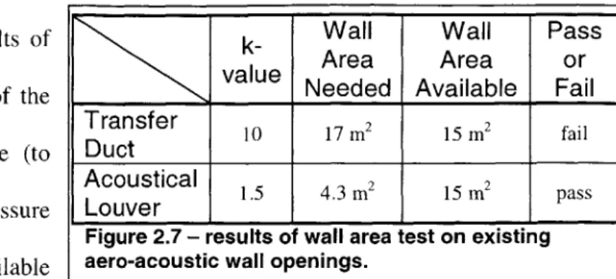
Using an adjusted k-value of 10 (and area ratio of 16%) for a typical transfer duct and a k-value of 1.5 (and area ratio of 25%) for a typical acoustical louver, the sample case (defined in chapter 1) illustrates how well each design will perform in a natural ventilation application. The following steps show the calculation process used to determine the required wall area for an aero-acoustic wall opening, and ultimately determine whether it meets the airflow design goal. The calculation assumes an airflow rate of lOACH and an overall pressure gradient of lOPa, then solves for the wall area required by the aero-acoustic device:
EXAMPLE: Findinq Wall Area Required by Aero-Acoustic Wall Openings
The total pressure gradient across all four walls is 10 Pascal. Assuming an even pressure-loss distribution, each wall will cause 2.5 (10 divided by 4) Pascal of pressure drop.
Knowing the k-value of the aero-acoustic wall openings in each wall (k = 10 for the transfer duct and 1.5 for the louver), the velocity through each opening is defined by:
2AP
pk
where:
AP = pressure loss through each wall (1.5 Pa),
u = average velocity through the cross section area of the opening, m/s, 3
p = air density, kg/m,
k = pressure loss coefficient.
The total occupied wall area for each wall is determined by the volume flow rate and the area ratio. The volume flow rate is defined by:
* ACH
3600
where:
V = total volume (450 M3),
V = volume flow rate through apartment, m3/s, ACH = air changes per hour (10).
Finally, the total area occupied by the aero-acoustic wall openings is defined by:
A =
u(area - ratio)
where:
A = total occupied wall area (in each wall), M2,
Figure 2.7 shows the results of k- Wall Wall Pass
Figur Area Area or
the above calculation in a table of thevalue Needed Available Fail Transfer 10 17 m2
15 m2
fail
wall area required by the device (to Duct _
Acoustical 1.5 4.3 m2 15 m2
pass
pass
lOACH
with alOPa
pressure Louver __I IFigure 2.7 - results of wall area test on existing
gradient) versus the wall area available aero-acoustic wall openings.
in each wall of the reference case. The transfer duct requires more wall area (17m 2) than is
available (15m2) so it fails, while the acoustical louver requires less wall area than is available in
each wall so it passes.
An aero-acoustic wall opening that meets both the airflow and the acoustic design goals must carefully balance the contradictory requirements of blocking noise and permitting airflow. Along with modifying the two existing designs, the process included brainstorming for new ideas.
2.4 DESIGN IDEAS
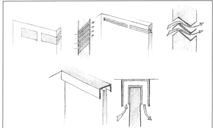
New design ideas evolved from the existing product designs (acoustical louvers and transfer duct). Figure 2.8 shows just a few of the ideas conceived during brainstorming. The two designs showing the best promise for both airflow and acoustic performance are the transfer duct (modified for improved airflow) and the U-shaped duct (shown in the lower part of figure 2.8). The design process then expanded the two design ideas and modified them to meet both th e airflow and the acoustic design goals.
The design of an aero-acoustic wall opening must evolve from an understanding of how it will perform as several variables change simultaneously. Acoustic and fluid mechanic theory combined with empirical data in the following section provide prediction models for noise transmission loss and airflow resistance of the two designs noted above.
2.5 ACOUSTIC PREDICTION
Complex acoustic theory could predict the exact transmission loss through an aero-acoustic wall opening (Ver, Scott, Beranek, Mechel, et. al.), but would require a detailed analysis with complex math and exact material properties not covered in this thesis. Instead, empirical methods for each component of the opening (entrance, bends, and straight duct) superimpose onto one another giving an estimate for the transmission loss through the entire opening (the noise attenuation through the solid wall, perpendicular to the duct, is so much larger than through the open duct, that it may be ignored). Chapter 4 presents revised prediction methods derived using the experimental results (the methods below were used to get a "first-cut" estimate so that test prototypes could be built).
Both designs have these three common duct components: an entrance and exit, one or two lengths of straight lined duct, and two bends. Beranek and Vdr (1992) propose a simple method for finding entrance and exit losses according to the graph in figure 2.9 (where the sound reduction, dB, at the entrance or exit is a function of wavelength, X, and cross-sectional height, h). Lippert
(1954) proposed an experimental validation of theoretical acoustics to find the sound loss
through a 90 degree bend, due to end reflections, though his method does not apply to these aero-acoustic designs because of the short
10 entrance and exit regions surrounding 8
their bends (analysis in Chapter 4 t
Uj 3
shows that this loss may, in fact, be
2
as shown in Chapter 4, that the lined duct portion of the designs contributes almost exclusively to the overall sound transmission loss.
According to Kuntz and Hoover, equations 5 and 6 predict the transmission loss of a straight duct with acoustic lining on all sides:
a 0.748h0.356 (P/A)L f (1.17+K2d)
TL - K dB (125 Hz < f < 800 Hz) (5)
TL K4(P/A)L f 1 log(P/A)) dB (800 Hz < f < 10,000 Hz) (6) W2.3h 2.
where,
ao = normal random absorption coefficient of the lining (not incident absorption), h = smallest inside cross-section dimension (mm)
P = inside cross-section perimeter (mm) A = cross-section area (mm2)
L = length of duct (m) f = frequency (Hz)
d = density of lining (kg/m3)
w = larger cross-section dimension (mm)
K, = 0.0214
K2 =0.19
K4 = 3.32E18
K5 = -3.79
The above prediction model is empirical and is, therefore, limited in application to test cases similar to those tested in the experiments. Testing of the formulae reveals that the curve becomes discontinuous if the aspect ratio (w/h) is large (Kuntz and Hoover base their method on tests of three cross sections with a maximum aspect ratio of 2).
Theoretically, transmission loss in a duct is linearly proportional to length and lined perimeter, and inversely proportional to cross sectional area:
TL= L (7)
the properties of the lining, the sound frequency, and the air temperature. Kuntz and Hoover maintain this relationship in their prediction method, using two complex equations for Ogeometry in each frequency range. Obviously, then, the goal is to maximize length and perimeter while minimizing cross sectional area. Further, according to Kuntz and Hoover, designs should also use a lining with low density and a large absorption coefficient.
It is not enough, however, to design an aero-acoustic wall opening that only optimizes sound transmission loss (if that were the case, a solid wall would suffice). Instead, the two designs must strike a balance for airflow and acoustic performance so that they meet both design goals. 2.6 AIRFLOW PREDICTION
The two designs comprise these four components: an entrance, an exit, one or more bends, and one or more lengths of straight lined duct.
Pressure loss for incompressible fluid flow through a duct system is the sum of the pressure losses through each component of the system, assuming the components are spaced far enough apart so that their streams do not mix (i.e. - entrance, exit, length of straight duct, bend, expansion, contraction, etc.):
APt = k pU2 (8)
i=1-*n
where:
AP = total pressure loss through all components of the duct system, Pa, n = number of components in the duct system,
Ui = mean velocity through the cross section at each component, m/s, ki = kiocai + kffiction = overall pressure loss coefficient for each component, kiocai = local dynamic pressure loss coefficient,
kffiction = viscous pressure loss coefficient,
compiled an expansive set of empirical pressure loss data for various duct components and geometries. The results of his work are "sufficiently basic to allow application to nearly any shape of flow passage encountered in engineering practice," (Editor's preface to the third edition). Simple addition of the pressure loss coefficients for each component provides, with limited accuracy, an estimate of the overall pressure loss coefficient through the duct system. The data provides a first-order understanding of how geometry will affect the overall airflow performance of the transfer duct and U-shaped duct. This analysis refined and verified in chapter 3 by a computational fluid dynamics (CFD) analysis.
Transfer Duct
For the transfer duct, the sum of three component pressure losses indicates the overall pressure loss: dynamic pressure loss at an entrance that immediately goes into an angle, friction pressure loss of a straight duct, and dynamic pressure loss at an exit that immediately follows a bend. The data below describes the losses as functions of duct geometry.
Entrance Component (into an Angle)
The entrance into the transfer duct is approximately the same as an entrance that is flush and at an angle of 20 degrees with the wall as shown in figure 2.11 (20 degrees is the smallest angle tested). The aspect ratio, w/h, is the variable of interest (h is the height of the opening in the plane of the bend, and w is the width of the opening).
As seen, a large aspect ratio (w/h) gives a lower pressure loss coefficient. This estimate for entrance loss,
-t H
w/h 25 1 0.5 0.2
k (at 20 degrees) 0.85 0.96 1.04 1.58
however, is a likely source of error since the actual geometry of a transfer duct entrance (i.e. - a sharp bend) is not an angled inlet.
Straight Duct Component (friction)
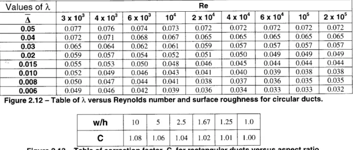
Similar to the commonly used Moody chart, Idel'Chik has assembled data for the pressure loss coefficient of ducts as a function of roughness, Reynolds number, and hydraulic diameter. The duct lining has an equivalent sand grain roughness of approximately 2mm (derived from Johns Manville Corporation literature). The following equations assist in deriving the overall k-value from the charts below (figures 2.12 and 2.13).
kfriction - kD h Re= puDh Dh A P -A A = Dh where:
kfriction = viscous pressure loss coefficient through straight duct, L = length of duct, m,
C = correction factor for rectangular ducts,
A = function of Reynolds number and average surface roughness (in chart),
Re = Reynolds number,
U = average velocity through cross section, m/s,
g = dynamic viscosity, Ns/m2 Dh = hydraulic diameter, m, A = cross section area, m2
P = wetted perimeter, m,
Values of X Re A 3x10³ 4x10³ 6x10³ 104 2x10⁴ 4x10⁴ 6x10⁴ 105 2x10⁵ 0.05 0.077 0.076 0.074 0.073 0.072 0.072 0.072 0.072 0.072 0.04 0.072 0.071 0.068 0.067 0.065 0.065 0.065 0.065 0.065 0.03 0.065 0.064 0.062 0.061 0.059 0.057 0.057 0.057 0.057 0.02 0.059 0.057 0.054 0.052 0.051 0.050 0.049 0.049 0.049 0.015 0.055 0.053 0.050 0.048 0.046 0.045 0.044 0.044 0.044 0.010 0.052 0.049 0.046 0.043 0.041 0.040 0.039 0.038 0.038 0.008 0.050 0.047 0.044 0.041 0.038 0.037 0.036 0.035 0.035 0.006 0.049 0.046 0.042 0.039 0.036 0.034 0.033 0.033 0.032
Figure 2.12 - Table of k versus Reynolds number and surface roughness for circular ducts.
w/h 10 5 2.5 1.67 1.25 1.0
C 1.08 1.06 1.04 1.02 1.01 1.00
Figure 2.13 - Table of correction factor, C, for rectangular ducts versus aspect ratio.
Figure 2.12 shows that larger Reynolds numbers and larger hydraulic diameters give smaller values for k, and thus a smaller k-value. Further, smaller aspect ratios produce a slightly
smaller correction factor (figure 2.13).
Exit Component (after a bend)
For an exit that immediately follows a sharp 90-degree bend (figure 2.14), figure 2.15 gives the k-value as a function of the cross-sectional aspect ratio (w/h), and the height ratio.
Value of k w/h hin/hout 4.0 1.0 0.25 0.5 9.9 9.0 8.8 1.0 3.2 2.9 2.7 1.4 2.0 2.0 1.8 2.0 1.3 1.3 1.3 Figure 2.15 - Table of k-values for an exit component
immediately following a bend. Figure 2.14 - exit after a bend.
Overall, the exit losses of the transfer duct are most significant (compared to the other two components), and increasing the flow area at the exit bend by making its height twice that of the internal cross section will minimize the pressure loss.
U-Shaped Duct
For the U-shaped duct, four component pressure losses from Idel'Chik (1994) add to give the overall pressure loss: dynamic pressure loss at an entrance with one side tangent to the wall, friction pressure loss of the straight duct, dynamic pressure loss at a 180 degree bend, and dynamic pressure loss at an exit with one side tangent to the wall.
Entrance Component (along a wall)
Idel'Chik gives the pressure loss coefficient, k, for a duct mounted flush on a wall as 0.63 regardless of geometry (shown in figure 2.16).
Straight Duct Component
The straight duct component losses are the same as they are for the transfer duct, above. Bend Component (180 degrees)
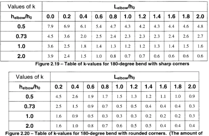
The pressure loss coefficient in a 180-degree bend depends on the geometry of the bends and whether the corners are sharp or rounded. Figure 2.17 shows the sharp bend and figure 2.18 shows the rounded bend. (hk in figure 2.18 is the same dimension as hei in figure 2.17.)
h
rF = e d/2
Values of k Lelbow/ho helbow/ho 0.0 0.2 0.4 0.6 0.8 1.0 1.2 1.4 1.6 1.8 2.0 0.5 7.9 6.9 6.1 5.4 4.7 4.3 4.2 4.3 4.4 4.6 4.8 0.73 4.5 3.6 2.0 2.5 2.4 2.3 2.3 2.3 2.4 2.6 2.7 1.0 3.6 2.5 1.8 1.4 1.3 1.2 1.2 1.3 1.4 1.5 1.6 2.0 3.9 2.4 1.5 1.0 0.8 0.7 0.7 0.6 0.6 0.6 0.6
Figure 2.19 - Table of k-values for 180-degree bend with sharp corners
Values of k Lelbow/ho helbow/ho 0.2 0.4 0.6 0.8 1.0 1.2 1.4 1.6 1.8 2.0 0.5 4.5 2.6 1.9 1.7 1.5 1.3 1.2 1.1 1.0 0.9 0.73 2.5 1.5 0.9 0.7 0.5 0.5 0.4 0.4 0.4 0.3 1.0 1.6 0.9 0.5 0.3 0.3 0.3 0.2 0.2 0.2 0.3 2.0 1.6 1.0 0.8 0.7 0.6 0.5 0.5 0.4 0.4 0.4
Figure 2.20 - Table of k-values for 180-degree bend with rounded corners. (The amount of rounding is a function of the other dimensions, shown in figure 2.18.)
Figures 2.19 and 2.20 show the k-values, as a function of duct geometry, for the sharp U-bend and the rounded U-U-bend, respectively. For both U-bends, it is critical to ensure that helbow is at least as large as ho. If the bend has sharp corners helbow/hO should be equal to 2.0 and Le1bow/ho
should be between 1.0 and 1.4. If the bend has rounded corners, heibow/ho should be equal to 1.0
and Lelbow/hO should be between 1.0 and 1.4. Under these conditions, rounded corners will halve
the k-value versus sharp corners (0.3 versus 0.7), but either case gives an adequately low k-value.
Exit Component (along wall)
While Idel'Chik (1994) does not specifically identify data for an exit along a wall, it will have a pressure loss coefficient no greater than about 1.0 (that of a standard open-duct discharge) and no less than about 0.5 (that of an optimum baffled exit). There is not much room for improvement at the exit without adding baffles, so the pressure coefficient of the exit will likely be closer to 1.0.
Chapter 3
Experiments
3.1 EXPERIMENTAL SETUP
Based on the acoustic prediction models the prototype designs should maximize duct length, cross-sectional aspect ratio, and the lining's absorption coefficient while minimizing the lining's density. Fortunately, the airflow prediction model indicates that a large cross-sectional aspect ratio will reduce pressure loss at the entrance and the straight duct components while not significantly increasing pressure loss at any other component, and that increasing duct length will only slightly increase pressure loss.
Two specific prototype designs emerge from the above results. Figure 3.1 details the U-shaped duct prototype (as-built) and figure 3.2
details the U-shaped duct prototype (as-built).
13" (0.33m)
For consistency, both prototype designs 3.5 (O.09m)
have the same cross-section dimensions and
use the same materials. Both have a cross-
h"
(O.13m) section with dimensions: h=2.5 inches43" (1.9m)%OpenArea43N(1.9*)(1" Zx 2.5") /(13" x 43") 3.5" 5 .3% (O.09m) 4.25 4 25" 13" (0.33m) -(0.06m) 12" (0.30 )- -1/2" Acoustic Lining (0.48m)
(0.0635m) and w=12 inches (0.3048m) as measured from the inside perimeter of the lining surface (giving an aspect ratio [w/h] of 5). The 'h' dimension is chosen so that the transfer duct will fit inside a standard 2"x4" stud-construction wall. The U-duct fits over the outside surfaces of the wall, so it does not need to be as narrow (though, for aesthetics, it should not protrude too far away from the wall). The combined length of straight lined duct is 3 feet (0.9144m) for both prototypes. Three-quarter inch chip board makes up the wall faces (its mass is similar to gypsum board, but is easier to work with during experiments); all ductwork uses sheet metal and is sealed with duct tape; " Permacoat Linacoustic lining by Johns Manville (found to have the highest absorption to density ratio of popular linings on the market) was attached to the ducts using adhesive "Stick-Clips ." Joints were sealed with "Diversi-GumT," a high-density clay-like compound, and covered with duct tape. Figure 3.3 shows the test section (seen from inside the source room) before the U-shaped duct prototype is installed.
According to the acoustic predictions, both prototypes should significantly fail to meet the design goal of a sound transmission class (STC) rating of 25 (see section 1.4 for a definition of STC). The predictions indicate an STC rating of only 8, because of poor predicted performance at higher frequencies. This, in fact, is not true, and experimental results reveal (in section 3.2) that the acoustic prediction method drastically under-predicts high frequency transmission loss, so the above result can be ignored for now.
The airflow prediction method indicates that the transfer duct will have an overall k-value of kentrance(0.85) + kfriction(O.5) + kexit(l.3) = 2.65. The open area of the transfer duct prototype is 4.6%. The U-shaped duct will have an overall k-value of kentrance(0.63) + kbend(O.7) + kfriction(0.5)
+ kexit(l.0) = 2.83. The open area of the U-shaped duct prototype is 12%.
When the predicted k-values are plugged into the reference apartment for airflow performance (detailed in section 2.1), the U-shaped duct will meet the airflow design goal (set in section 2.2), but the transfer duct will not. Figure 3.4 details the results ("wall area required" is the area occupied by the devices to pass 10 ACH with a total pressure gradient of IOPa). Further testing and investigation are necessary to fully understand the performance of both designs and to derive solid conclusions. Chapter 4, Refined Designs, further explores the designs and their performances.
Wall area
k- %open Wall area
value area required by available Pass/fail?
device Transfer 2.65 5.3% 18.9 m2 15 m2 Fail Duct U-shaped 2.83 12% 8.6 m2 15 m2 Pass
Duct
3.___mr _ f___rf__ predictinresu for __ ____"asbui _ _prottypes3.2 ACOUSTIC EXPERIMENTS 3.2.1 Procedure
Testing the noise transmission loss (TL) of the prototypes according to ASTM Standard E90-97 provides quantitative results of noise performance for the prototypes. BBN Laboratories in Cambridge, Massachusetts provided reverberant test chambers for the experiments. The facility comprises two "reverberant" rooms (a source room and a receiver room, each with minimal acoustic absorption) connected by a concrete wall with a removable section for mounting test specimens (figures 3.5, 3.7, and 3.8). A centrifugal sound source (Bruel & Kjaer type 4204, figure 3.6) creates a uniform sound field near 90 dBA (between 100 Hz to 10,000 Hz) in the source room. The sound travels through the test specimen into the receiver room where the room absorbs some sound while the rest produces a uniform sound field. A sound analyzer (B&K 2260 Investigator) measures the sound spectrum at six spatial points in the source room and at six spatial points in the receiver room (figure 3.5).
x ZZ
S FTEST SECTION
$3 R-4
56
Figure 3.5 - Plan Drawing of Test Chambers.
"S" points are microphone locations in the Figure 3.6 - B&K centrifugal sound source source room, and "R" points are microphone (type 4204) and its average spectrum as
The six measurements from each room are averaged at each frequency (logarithmically) to create an overall sound-pressure level in the source room (LI) and an overall sound-pressure level in the receiver room (L2). Equation 9 determines the sound transmission loss through the test specimen (at each frequency), based on the experimental data:
TL =< LI > - < L2 > +OLog(A/a) (9)
where:
TL = transmission loss at each 1/3-octave band, dB, <Ll> = average sound pressure level in the source room, dB, <L2> = average sound pressure level in the receiver room, dB,
2
A = wall area occupied by the device in the receiver room, m2
2
(X = sound absorption in the receiver room, m.
A time-decay experiment determines the sound absorption (a) in the receiver room by measuring how quickly a uniform sound field decays at each frequency after the sound source stops (the source room's absorption is not important to know because it only effects the sound field in the source room, which is measured directly). A sound analyzer (HP model 35670A) coupled with a speaker (using an 80-watt amplifier), a band-pass filter, and a microphone measured the decay rate (dB/second) of sound at each 1/3-octave band frequency. Appendix A contains time-decay data from the tests while figure 3.9, below, lists the decay rate and corresponding absorption (a) at each frequency.
The absorption in the room at each frequency relates to the time decay of sound in the room according to equation 10 (ASTM Standard E90-97):
a = 0.921 Vd (10)
C
where:
a = sound absorption in the room, m2 or Sabines, V = volume of the room, m3 (87.8 m3 in receiver room), c = speed of sound in air, m/s (343.3 m/s at 20'C), and