Saturation estimates for hp -finite element methods
23
0
0
Texte intégral
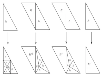
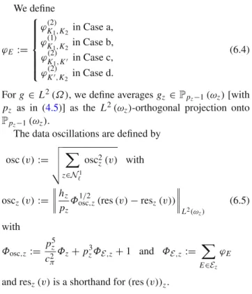
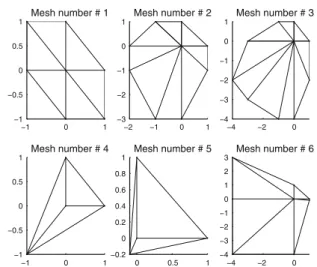
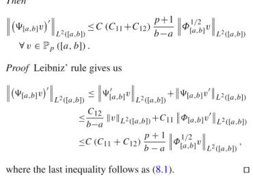
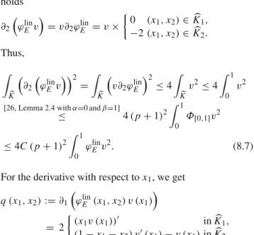
Figure
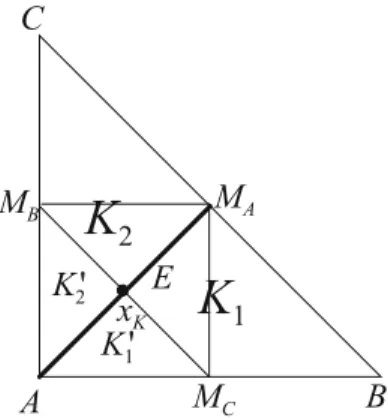
+4
Documents relatifs