HAL Id: cirad-00749814
http://hal.cirad.fr/cirad-00749814v2
Submitted on 8 Jan 2013HAL is a multi-disciplinary open access archive for the deposit and dissemination of sci-entific research documents, whether they are pub-lished or not. The documents may come from teaching and research institutions in France or abroad, or from public or private research centers.
L’archive ouverte pluridisciplinaire HAL, est destinée au dépôt et à la diffusion de documents scientifiques de niveau recherche, publiés ou non, émanant des établissements d’enseignement et de recherche français ou étrangers, des laboratoires publics ou privés.
Using a crop model to account for the effects of local
factors on the LCA of sugar beet ethanol in Picardy
region, France
Cécile Bessou, Simon Lehuger, Benoit Gabrielle, Bruno Mary
To cite this version:
Cécile Bessou, Simon Lehuger, Benoit Gabrielle, Bruno Mary. Using a crop model to account for the effects of local factors on the LCA of sugar beet ethanol in Picardy region, France. International Journal of Life Cycle Assessment, Springer Verlag, 2013, 18 (1), pp.24-36. �10.1007/s11367-012-0457-0�. �cirad-00749814v2�
1
Using a Crop Model to Account for the Effects of Local Factors on the LCA of Sugar Beet Ethanol in Picardy region, France
Cécile Bessou1, Simon Lehuger2, Benoît Gabrielle3, Bruno Mary4
1
CIRAD, Performance of perennial cropping systems research unit, Av. Agropolis, F-34398 Montpellier, France.
2
INRA, Environment and agricultural crop research unit, F-78 850 Thiverval-Grignon, France
3
AgroParisTech, INRA, Environment and agricultural crop research unit, F-78 850 Thiverval-Grignon, France
4
INRA, US1158 Agro-Impact, F-02 007 Laon-Mons, France
Corresponding author: Cécile Bessou, CIRAD, Avenue Agropolis, F-34398 Montpellier Cedex 5, France - Phone: +33 4 67 61 44 87 - Fax: +33 4 67 61 65 90
E-mail: cecile.bessou@cirad.fr
Key words: Biofuel, Ethanol, Sugar Beet, Local LCA, Greenhouse Gases, Agricultural Practices, Process-based Model, CERES-EGC, NOE2, N2O
Retrieve the publisher version at:
2 Abstract
Background. The results of published Life Cycle Assessments (LCAs) of biofuels are characterized by a large variability, arising from the diversity of both biofuel chains and the methodologies used to estimate inventory data. Here, we suggest that the best option to maximize the accuracy of biofuel LCA is to produce local results taking into account the local soil, climatic and agricultural management factors.
Methods. We focused on a case-study involving the production of first-generation ethanol from sugar beet in the Picardy region in Northern France. To account for local factors, we first defined three climatic patterns
according to rainfall from a 20-year series of weather data. We subsequently defined two crop rotations with sugar beet as a break crop, corresponding to current practice and an optimized management scenario, respectively. The six combinations of climate types and rotations were run with the process-based model CERES-EGC to estimate crop yields and environmental emissions. We completed the data inventory and compiled the impact assessments using Simapro v.7.1 and Ecoinvent database v2.0.
Results. Overall, sugar beet ethanol had lower impacts than gasoline for the abiotic depletion, global warming, ozone layer depletion and photochemical oxidation categories. In particular, it emitted between 28 and 42% less greenhouse gases than gasoline. Conversely, sugar beet ethanol had higher impacts than gasoline for
acidification and eutrophication due to losses of reactive nitrogen in the arable field. Thus, LCA results were highly sensitive to changes in local conditions and management factors. As a result, an average impact figures for a given biofuel chain at regional or national scales may only be indicative within a large uncertainty band.
Conclusion. Although the crop model made it possible to take local factors into account in the life-cycle inventory, best management practices that achieved high yields while reducing environmental impacts could not be identified. Further modelling developments are necessary to better account for the effects of management practices, in particular regarding the benefits of fertiliser incorporation into the topsoil in terms of nitrogen losses abatement. Supplementary data and modelling developments also are needed to better estimate the emissions of pesticides and heavy metals in the field.
3
1. Introduction
The development of renewable energy sources has recently been fostered and promoted as an alternative to the use of fossil resources to mitigate greenhouse gas (GHG) emissions and climate change worldwide (IPCC 2011). While no single renewable energy source may claim to be the perfect solution, it is their best combination in relation to local resources that may lead to a carbon neutral energy mix. Among these renewable sources, biofuels have been largely promoted worldwide. In Europe, the renewable directive (2009/28/EC, European Commission 2009) aims at substituting 10% of its fossil fuel consumption for transport with biofuels by 2020. In order to be eligible for this share and to benefit from fiscal incentives, biofuels should comply with a set of sustainability criteria, including minimum GHG savings of 35% compared to equivalent fossil fuels. These criteria were imposed to ensure a net benefit in terms of environmental impacts with biofuels, following the controversy on their life-cycle GHG emissions (Quirin et al. 2004; Farrell et al. 2006).
Life Cycle Assessment (LCA) is the most commonly-used framework to assess the environmental impacts of products throughout their life cycle, since its holistic approach makes it possible to avoid pollution trade-offs across the life-cycle stages or impacts. However, the complexity of biofuel chains has evidenced some limits of this methodology, in particular because system boundaries are variable across studies, and because the
assumption that emissions are proportional to inputs is often violated for field emissions. These emissions result from complex biogeochemical processes that are strongly dependent on local soil, climatic and management factors. For instance, the emissions of nitrous oxide (N2O), a gas with a global warming potential 298 times
larger than CO2 (Forster et al. 2007), depend on a number of the above-mentioned factors and are therefore
highly variable at the plot scale (Parkin 1987; Mosier et al. 1996; Farquharson and Baldock 2008). As a consequence, the linear regression model used in the IPCC Tier 1 (2006) estimation method, which only accounts for soil N input rates should only be expected to provide an order of magnitude for these emissions, associated with a wide uncertainty band (-70% to +300%; IPCC, 2006).
Also, many studies on biofuel chains are focused on specific impacts (e.g. global warming) rather than the range of impacts that may be potentially addressed by LCAs (Quirin et al. 2004; Blottnitz and Curran 2007), thus conveying an incomplete picture of biofuels sustainability. Finally, given the expanding demand for biofuels and the limited available land area, concerns have risen that biofuels may lead to land use changes, whose impacts are not yet fully assessed within the classical (attributional1) LCA framework (Reinhard and Zah 2009). Because of all these limitations of LCA, confusion and controversy arose on the environmental interest of biofuels (Crutzen et al. 2008; Fargione et al. 2008; Bessou et al. 2010a).
Assessing the environmental impacts of a biofuel chain with enough accuracy so that a decision can be made with respect to the above-mentioned sustainability criteria requires: 1) the definition of common system boundaries and methodological choices; and 2) a reduction of the uncertainty of inventory data, which may be achieved by more accurate emission models. There are currently ongoing international projects seeking to harmonize the LCA methodology (PAS2050 by BSI 2008; ISO 140672; ILCD by European
Commission-JRC-1
An attributional LCA is a descriptive LCA assessing the impacts of an added produced Functional Unit = FU (status-quo + FU) without considering the changes induced by this added FU as it is done in a consequential or change-oriented LCA (FU + consequential modifications of the initial state due to the added FU).
2
4
IES 2011), while past studies have dealt with system boundaries for biofuel chains (Quirin et al. 2004; Farrell et al. 2006). Other studies also used agro-ecosystem models to generate input data for the life-cycle inventory, thereby reducing the uncertainty of emissions from agricultural fields (Gabrielle and Gagnaire, 2008; Langevin et al. 2010). Nevertheless, these model outputs were either specific to a set of particular sites (for the latter studies) or related to country averages in terms of management data (JRC 2008; Smeets et al. 2009). When dealing with biofuels, data representative from the feedstock supply area should be sought.
Our objective was hence to produce such a 'local LCA' for first generation ethanol from sugar beet, and to test the sensitivity of its results to changes in local environmental or management factors. We used the Picardy region in Northern France as a case-study, involving sugar beet as a feedstock. Sugar-beet has been produced on a large scale for decades in this area. To account for in the effect of local factors, we simulated crop growth and N emissions to the environment with the dynamic agro-ecosystem model CERES-EGC (Gabrielle et al. 2006). This works addresses regional variations and data quality but does not address inconsistency in system boundary and the linearity assumptions imposed on the parameters not modelled.
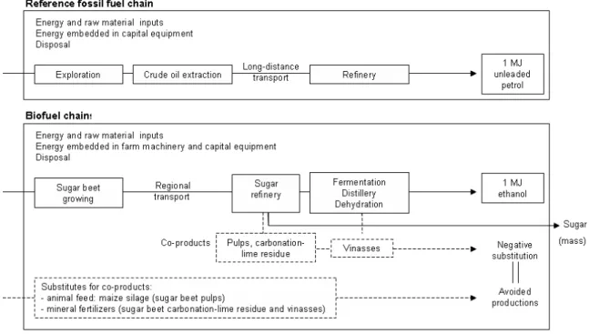
2. Material and Methods 2.1 Goal and system boundary
The aim of this study was to conduct a full-blown attributional Life Cycle Assessment of the production and combustion of first-generation ethanol from sugar beet. We compared ethanol from sugar beet with its fossil-based equivalent, gasoline, to examine the benefits of substituting the latter with bio-ethanol, however strictly in an attributional framework. System boundaries were Well-to-Tank, i.e. including all flows of resources, energy and pollutants from the extraction of raw materials up to ethanol dehydration. The chosen functional unit was 1 MJ of biofuel energy content, using the low heating value (LHV) of ethanol. This was calculated from the potential energy that would be delivered by the fuel at the refinery gate if its combustion in the car engine was complete. Since we focused here on the impacts of biofuel production and more specifically on its agricultural feedstock, we did not include the steps of fuel blending and distribution to the filling station, as both would be similar between the two fuels. Energy embedded in farm machinery and capital equipment was included. On the contrary, the caloric intake and transportation of farm workers were not included (Farrell et al. 2006). Missing reliable inventory data prevented a complete inventory of some packaging, enzyme and yeast inputs for the fermentation processes. In terms of land use, we considered that sugar-beet was grown on existing crop land, so that no land-use changes occurred (PAS2050 by BSI 2008). From an attributional perspective, we assessed the impacts of producing sugar beet ethanol without accounting for any possible displacement of other crops to compensate for the resulting reduction in sugar production. This approach was in accordance with the underlying assumption that there is an over-production of sugar in this region, as a result of the sugar reform in the
European Union. We did not account for biogenic CO2 fixation and emissions since no emissions from land use
change were considered. The system boundaries for the two fuel chains are presented Figure (1).
The system was extended to take into account savings due to the substitution by co-products as recommended by LCA-ISO standards (ISO 14044:2006). Over the year, sugar beet ethanol is produced from different raw
materials: sugar-beet juice and fermentation slurry during the campaign (in the 3 months following the harvest of sugar-beet crops), and syrup and slurry during the remaining time interval (inter-campaign). The inputs and
5
outputs of the refinery-distillery processes were calculated based on the mass balances of the processes from raw material to the various final products over the year. The co-products of sugar beet ethanol considered included pulp, lime-carbonation residue, vinasse and sugar. For each of these co-products, alternative chains were designed according to local practices and the expertise of professionals from the region. The avoided production of mineral fertilisers was calculated based on the chemical composition of co-products and their mineralization rates, depending on the site and time of spreading (Decloux et al. 2002; ITB 2002). The equivalent of pulp was silage maize, given the close dry matter contents (around 25% DM) and low protein values of the two products that leads farmers to use them indifferently in feeding rations (Comité National des Co-Produits/ADEME 2002). In state of the art of sugar beet sugar-and-ethanol production plants in France, sugar represents the main output. For the allocation between sugar and ethanol, we intrinsically used a mass-based procedure through the mass balance calculation. It is justified by the fact that the only locally-available substitute for sugar involved the same sugar-beet chain. Given this case, the use of system expansion and from mass-based allocation would give the same results.
2.2 Temporal and geographical scopes
LCA typically provides a “snapshot” of the studied systems at a given point in time. Here, the reference period for the data related to industrial processes was the 2000-2010 time interval, i.e. involving state-of-the-art technologies currently in use at commercial level. No prospective scenarios involving possible near-term improvements over these technologies in terms of energy efficiency or pollution abatement were analysed. In particular, we did not consider any possibility of capturing fermentation-derived CO2. The reference period for
agricultural productions was the 1988-2009 time interval to account for sufficient climate variability in the modelling work. Crop management data were representative of a more recent period running from 2000 to 2010.
The agricultural production site considered was the INRA Agro-Impact experimental station at Estrées-Mons in the Picardy region (49°80’N, 3°60’E), where the mean annual precipitation and air temperature are 667 mm and 9.6°C respectively (Guérif et al. 1996). The size of the experimental site is 170 ha. The annual total sugar beet area represents 15 ha. The soil is an Orthic Luvisol (FAO, 1998), which represents 20% of the arable soils in this region (Gagnaire et al. 2006). In order to better capture the emission variability due to the local production factors, climatic and agricultural management data were collected from this station over 21 years. In this area, sugar beet is a common break crop rotated with wheat and maize. None of these crops are usually irrigated.
2.3 Life cycle inventory of the agricultural production 2.3.1 Sugar beet cropping system
Field emissions are linked to physico-chemical and microbial transformations in soils. They can be classified as direct or indirect according to their occurrence in the causal chain from the application of agricultural inputs to the final impacts incurred. For instance, primary emissions of leached nitrate are defined as direct field emissions, whereas N2O emissions ensuing from this primary emitted nitrate but occurring beyond the
agricultural field itself are considered indirect. Field emissions are related to reactive compounds either applied to the field as fertilisers and pesticides, or originating from the mineralization of crop residues. Most field-applied fertilisers and pesticides are managed over one crop cycle. However, some fertilisers such as lime may
6
be managed at the crop rotation level. In our case study, lime was managed over a 4-crop rotation, hence one fourth of the input rate and spreading costs were allocated to sugar beet.
In order to account for all field emissions, we considered sugar beet as part of the sugar beet-winter wheat-maize-winter wheat rotation, which is common in the area. This rotation was implemented and monitored at the study site for more than 20 years. We simulated this rotation with CERES-EGC during the 1988-2009 time period, meaning that each run consisted of 5 repetitions of the rotation. To obtain an occurrence of sugar-beet for all individual years of the 1988-2009 period, we shifted the starting year from 1988 to 1991, resulting in four model runs. For all crops, residues were incorporated by deep ploughing. Emissions due to residue
mineralization and nitrate leaching were allocated to each crop of the rotation by considering that N
mineralization was the main source of inorganic N in between two growing seasons. We first defined the time interval for this allocation as the period running from the sowing of the crop of interest to the first fertiliser application on the following crop. In terms of tillage, each crop was thus allocated the incorporation of its harvest residues. Since the studied rotation included some 8 months of bare soil between wheat harvest and the sowing of sugar beet or maize, we allocated part of this bare soil period to these spring crops. This
discrimination resulted in a final splitting of the whole rotation into four one-year periods, starting and stopping on February 15th each year. N-inputs were calculated from a balance of crop requirements and supply from soil, including residue returns from the preceding crops. Hence, the green residues from sugar beets left in the field after harvest were not considered as a co-product of ethanol in the LCA.
The current crop rotation is not optimal in terms of soil cover. Introducing a cover crop between winter wheat and sugar beet, for instance, may reduce the bare soil period by some 85 days (ITB 2002). This cover crop is thereby expected to reduce N-losses by taking up N prior to the winter drainage period, and to make it available to the following crop after the cover crop has been ploughed in. The combined effect of cover crop on reducing nitrate leaching and increasing efficiency of N-uptake by the crops can be significant over the years (Constantin et al. 2010). N-losses may be further reduced by adjusting fertiliser N management. In particular, the soil incorporation of the first fertiliser N application together with the seeds can save as much as 15 kg N ha-1 yr-1 (ITB 2002). Beside our baseline scenario of the current rotation, we hence tested an “optimized rotation”, consisting of 2 aspects: 1) the introduction of a cover crop within the rotation between winter wheat and sugar beet or maize; and 2) the incorporation of N inputs upon sowing allowing the above mentioned savings of 15 kg N ha-1 yr-1 in both sugar beet and maize fields. In the study, we extended the cover crop, i.e. mustard, from August 15 until January 5, i.e. 144 days, so that it would be killed by the frost without requiring herbicides. The consequences for sugar-beet were accounted for through the resulting decrease of N losses between February 15th and the sowing in April as simulated by the crop model. The costs of cover crop establishment, i.e. sowing and mechanical destruction were equally split between sugar beet, winter wheat and maize. Annual P and K fertilisation rates in sugar beet plots were 70 kg ha-1 P2O5, and 110 kg ha-1 K2O. These inputs, as well as
pesticides and tillage operations (except for the introduction of the cover crop) did not vary between the two management scenarios. N-fertiliser rates and modelled yields are shown in Table 1.
7
To take into account local soil and climatic factors in the LCA, we modelled feedstock production with the agro-ecosystem model CERES-EGC (Gabrielle et al. 2006). This process-based model simulates crop growth by considering the type of soil, climate conditions, plant variety, and management practices at the field scale. It also predicts substance losses outside the ecosystem such as nitrate leaching, ammonium volatilization (Génermont and Cellier 1997), and nitrous oxide emissions through nitrification and denitrification which are predicted with the NOE model (Hénault et al. 2005). In order to improve its accuracy, we implemented the NOE2 sub-model (Bessou et al. 2010b) in CERES-EGC and proceeded to a Bayesian calibration of the 22 parameters of NOE2. This calibration makes it possible to reduce significantly the spread in parameter distribution and the subsequent uncertainty on N2O emissions by updating these distributions against a priori probability distributions
of parameter values gathered from other sites (Lehuger et al. 2009). This calibration reduced the Root-Mean Square Error on daily and annual fluxes by 15% and 63% respectively when compared to the uncalibrated simulations (Fig. 2), based on experimental data collected in our study site over sugar-beet (Bessou et al., 2010b). Calibrated parameters were then used for the simulations of sugar beet cropping system with CERES-EGC (Leviel et al. 2000; 2003). Despite our efforts, CERES-CERES-EGC still underestimated emissions in 2008-2009 due to several combined factors (Bessou et al. 2010b). Other sources also showed a marginal error of roughly 20% with CERES-EGC (Hénault et al. 2005; Gabrielle et al. 2011). This error remains lower than the uncertainty associated with IPCC factors.
We used daily climate data from a weather station located on site, and input soil and management data for the 21-year simulation period (1988-2009). According to climate records over this period and annual rainfall, we identified 3 climate patterns: 1) median years (R50; there were 9 years in this class in the simulation period), 2) inferior quartile years, “drier” than median years (R25; 5 years), and 3) superior quartile years, “wetter” than median years (R75; 5 years) (Fig. 3). Average values (arithmetic means) of modelled yields and emissions were calculated for the 6 combinations of rotation management and climatic years, noted R25, R50, and R75 for the baseline crop rotation, and R25 optim, R50 optim, and R75 optim for the optimized crop rotation. The resulting data are given in Table 1, and were fed into the life cycle inventories. An overview of the study approach and tested parameters is given in Figure 4.
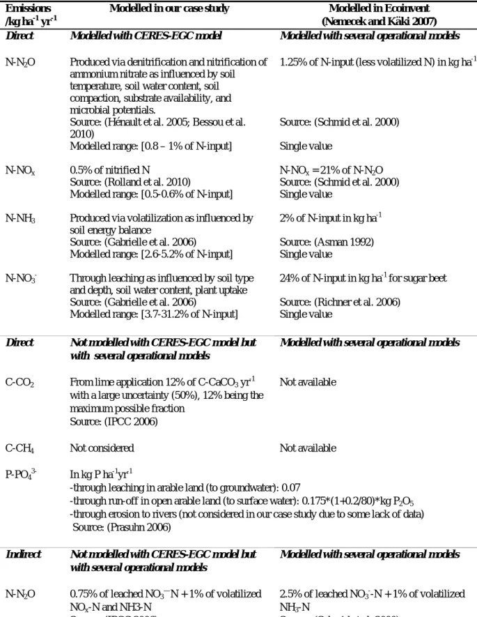
2.3.3 Field emissions not modelled with CERES-EGC
Changes in the spatial and temporal scales between direct and indirect field emissions make it particularly difficult to assess indirect emissions. Mechanisms are poorly characterized and indirect emissions are therefore not modelled by CERES-EGC. We thus used IPCC coefficients as an alternative to estimated indirect emissions, and also to estimate CO2 emissions due to lime application.
Methane emissions are not considered by CERES-EGC, but were ignored since the soil was well-drained and unlikely to be a net emitter or consumer of CH4 (BIOIS 2008). Finally, we accounted for heavy metals brought
to the soil by fertilisers following the corresponding inventory method of Ecoinvent. Due to the lack of reliable data on the heavy metals brought to the soil in pesticides or exported with the harvested biomass, we decided not to account for them. The modelling of direct and indirect emissions linked to agricultural productions in this
8
study in summarized in Table 2, also showing the differences with their respective models in the Ecoinvent3 documentation (Nemecek and Kägi 2007).
2.4 Life cycle inventory of the industrial phase
Background data on primary energy sources, infrastructures, machines, industrial production and disposal were mainly taken from Ecoinvent v2.0 databases (Swiss Centre for LCI). We used the data provided on the average French mix for electricity from the grid, as well as European average data for crude oil supply, oil refinery and energy embedded in infrastructures and machines. Transports of inputs to the agricultural field encompassed that of co-products from the refinery to the field, as well as saved transports for the products they substituted, except for maize silage which was produced on farm. Transport distances corresponded to current practices at the study site: 65 km for the supply of agricultural inputs to the farm, 22 km for the transport of sugar-beet roots to the sugar refinery, and 200 km for the other inputs of the refinery. Conversion data was taken from the Arcis-sur-Aube sugar refinery-distillery, which is located in the Champagne-Ardennes region neighbouring Picardy. This refinery-distillery is representative of the state of the art of such production units in France (ADEME 2010).
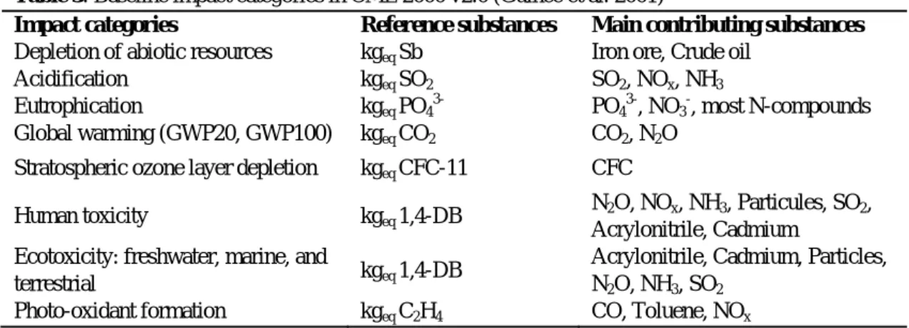
2.5 Impact characterization
We used the CML 2000 Baseline v2 method (Guinée et al. 2001) for the impact characterization, similarly to the reference LCA study commissioned by the French Environment Agency (ADEME, 2010). CML 2000
encompasses the impact categories listed in Table 3. Impact indicators were not subsequently normalized or weighted since these steps are partly subjective and uncertain, and hamper the interpretation of the LCA results (Guinée et al. 2001). Weighting in particular is not allowed by LCA-ISO standards when publicly comparing products, which is our objective here. LCA calculations were carried out with the SimaPro 7.1 software (PRé Consultants bv, NL).
3 Results and discussion 3.1 Biofuel versus fossil fuel
Figure 5 compares the environmental impacts of the production and the pseudo complete combustion of sugar beet ethanol and gasoline (low sulphur grade) on a MJ basis. Six scenarios of sugar beet ethanol productions were compared, corresponding to the six combinations of climate patterns (3) and crop rotations managements (2). Overall, the impacts of sugar beet ethanol were lower than those of gasoline in four categories: abiotic depletion, global warming, ozone layer depletion, and photochemical oxidation. Conversely, gasoline outranked bio-ethanol for acidification, eutrophication, human toxicity, and fresh water or terrestrial ecotoxicity. Feedstock production contributed more than 75% of total impact indicators for acidification and eutrophication for ethanol, with emissions of reactive N from fertiliser inputs in the field being the top contributors. Despite substantial reduction in nitrate leaching with the optimized rotation (Table 1), field emissions dominated the eutrophication impact. Reactive N also contributed to a large extent to GHG emissions in the field, while agricultural
production contributed 25% to 68% of the other impact categories. The industrial conversion processes
contributed to a large extent (more than 55%) to abiotic depletion, ozone layer depletion, aquatic ecotoxicity and
3
The ecoinvent Centre - a Swiss Competence Centre of ETHZ, EPFL, PSI, Empa and ART - is the world's leading supplier of consistent and transparent life cycle inventory (LCI) data of known quality with the database ecoinvent data v2.2. See http://www.ecoinvent.ch/
9
photochemical oxidation. Across impact categories, transport only contributed to 5 to 10% of total impact indicators.
Sugar beet ethanol produced in Picardy lead to savings of 28-42% greenhouse gases and 20-28% fossil resources compared to gasoline, on a MJ basis. The mean GHG emissions across scenarios amounted to 5.78 10-2 kg CO2
eq per MJ, corresponding to a 35.7% of GHG saving compared to gasoline. These emissions are larger than the France-wide average than those reported for sugar beet ethanol by ADEME, at 3.04 10-2 kg CO2 eq MJ-1
(ADEME 2010), but close to the European average value of 5.75 10-2 kg CO2 eq MJ-1 published by JRC
(2008), where sugar beet pulp was also used as cattle feed. Across our 6 feedstock scenarios, the global warming, eutrophication, and human toxicity indicators laid within -51% and +113% of the ADEME study (2010). Global warming impacts were all higher than ADEME (2010) (+80% to +113%), as well as human toxicity impacts (+24% to +52%), while eutrophication impacts were either lower (-51%) or higher (+23%) depending on the feedstock scenario. However, both studies are not directly comparable due to differences in system boundaries and field emission models, and scope. The ADEME (2010) and JRC (2008) estimates apply to national to continental scales and are relevant to public policies at macro-economic level, while our results were more local and targeted at stakeholders such as farmers or chain operators in the region. The sensitivity of LCA results to local factors highlights the relevance of this local LCA to define strategies at this level.
In our study, the conversion of one-hectare sugar beet provided between 2.60 and 3.97 t ethanol across the scenarios, since ethanol only made up 35% of the total outputs from the sugar refinery-distillery. Should this ratio rise to 100%, as assumed in the JRC study (2008), ethanol yields per ha would be nearly twice as high (at 5.78 t ha-1 - ADEME/DIREM, 2002). Because the data collected from the sugar refinery-distillery were
aggregated across the ethanol and sugar end-products and both chains were tightly entangled, it was impossible to test such a scenario and subsequently apply an energy-based allocation between ethanol and its remaining co-products, as recommended in the European Renewable Directive (RED) methodology (2009/28/EC, European Commission 2009). At any rate, this scenario would not be representative of the current situation, since
industrial processes have been up to now optimized to reduce energy costs for the combined production of sugar and ethanol during both campaign and inter-campaign periods. Moreover, sugar has a higher added-value than ethanol, making the 100% ethanol unrealistic. To our understanding, this duality was not considered in the RED methodology. Despite its particular configuration, sugar beet ethanol in Picardy would comply with the RED requirement of 35% GHG savings. Further conversion of the current sugar co-product to ethanol would indeed lead to higher ethanol yields per hectare with identical field emissions, and consequently lower GHG emissions per MJ of ethanol. Nevertheless, our results pointed out though that considering local factors, when data is available, might be crucial and more relevant than default parameters from the RED guidelines.
Since assessing the life-cycle GHG emissions of biofuels is essential from a policy standpoint, we examined its sensitivity to the global warming potential (GWP) of GHGs. We found an inconsistency between the value used in the JRC (2008) report and that reported in the RED e methodology description (Annex V.C), both cited by the same Directive. This was also reported in the Biograce calculator (IE 2011). These sources used GWP values (for a 100-year horizon) of 23 kg CO2 eq per kg CH4 and 296 kg CO2 eqper kg N2O (IPCC 2001) or
25 kg CO2 eq per kg CH4 and 298 kg CO2 eq per kg N2O (IPCC 2007). In our calculations, there were actually
20-10
year period (considering higher concerns for immediate consequences and action needs) had a more visible effect. For the R50 scenarios, for instance, the largest differences occurred between the 20-year (2007) and 100-year (2001) perspectives, with GHG emissions of 6.20.10-2 and 5.70.10-2 kg CO2 eq per MJ, respectively. This
difference would correspond to either 32.6% or 36.8% greenhouse gas savings compared to gasoline, respectively. We completed this sensitivity analysis by halving the CO2 emission factor of applied lime, as
suggested in the IPCC Guidelines (2006), but it only had a marginal effect on GHG budgets. Sugar-beet development is sensitive to pH and to a risk of surface crust in the soil of Estrées-Mons, so that liming must be carefully managed. In our study site, the liming rates were minimal because of regular lime applications in the past. However, in the cases of soils with higher risks of surface crusting or insufficient liming record, rates could easily double and the consequences on global warming impact become more important. This factor should be accounted for while identifying the best locations and managements for sugar-beet farming.
3.2 Impact of local production factors
LCA results were sensitive to changes in climatic conditions during biomass production. As detailed in Table 1, local production factors influenced fresh matter yields, but also all N-emissions that contribute to several impact categories. Consequently, local factors also had an influence on the final impacts. Compared to the sugar yields recorded on site over the 1990-2008 period, modelled yields were higher but with a larger standard deviation across years, but within the same order of magnitude as the observed yields. The observed yields as averaged over the drier, median and wetter years amounted to 78, 78 and 81 tonnes per hectare (standard deviations: ± 11-13%), compared to modelled yields of 76, 95, and 96 tonnes per hectare, respectively (standard deviations: ± 15-44%) (Table 1). Climatic patterns affected impacts across categories and management scenarios with a
maximum relative difference of about 60% in terms of GHG savings and an average difference per impact around 15% (Fig. 5). The largest difference occurred with eutrophication between the R25 and R50 climates.
Drier years (R25) were more radically distinct from the other climates, and had the largest standard deviations, indicating a higher uncertainty in dry years. On a hectare basis (Fig. 6), the impacts of sugar beet ethanol under the R25 climatic pattern were lower than for the other patterns, whatever the impact category. Drier years resulted in lower direct emissions of all N-compounds and subsequent indirect emissions, leading to reductions in the eutrophication, acidification, and global warming impacts. However, drier years (R25) were also
characterized by lower biomass yields and ethanol ethanol production per hectare. Ethanol yields (kg) were 20% lower on average for the R25 scenario compared to R50 and R75, the latter showing similar ethanol yields per hectare (±2%). On a MJ basis (Fig. 5), R25 ethanol had therefore higher environmental impacts, except for eutrophication, which was the most sensitive to rainfall patterns. In the drier years (R25), nitrate leaching was on average eight times lower than in the other years. Between the R50 and R75 scenarios, differences also appeared for the acidification and eutrophication impacts, which emphasize their sensitivity to climatic conditions.
When comparing baseline and optimized cropping systems on a MJ basis, the impact reductions between ethanol and gasoline varied from 10% to 45% across impacts (Fig. 5). The largest difference occurred for eutrophication between R50 and R50 optim. The introduction of a cover crop reduced nitrate leaching more efficiently during median years (R50 optim) than during drier (R25 optim) or wetter years (R75 optim). Across impact categories and scenarios, the optimized rotations had higher impacts, except for acidification (in the drier years) and
11
eutrophication (in the median to wet years). However, robust conclusions on the comparison of both rotations could not be drawn because of the trade-off between yield levels and field emissions, resulting in inconsistent rankings across impact categories. On average, yields were 16% lower with the optimized scenarios because of the reduced fertiliser inputs. The lower yields counter-balanced the lower field emissions occurring with the optimized system, which is a result of the strategic choices behind the optimization of the crop rotation. The latter implicitly considered land area as the main constraint for resource preservation: reducing fertiliser inputs per hectare aimed at abating N losses, while shortening the period under bare soil was expected to reduce nutrient losses. Yield optimization was therefore not a major factor in the management design although they certainly were in the LCA. This emphasizes the need to factor in ecological intensification targets when designing agricultural strategies, to avoid potential extensification and consequential increases in agricultural land area where land area is a limiting factor. This study, however, does not consider consequential impacts.
The lower yields with optimized systems may be also partly attributed to a modelling artefact. Indeed, the relative benefit from topsoil fertiliser incorporation at sowing could not be modelled since CERES-EGC considers that fertilizer N is always incorporated into the topsoil. It is thus likely that the baseline scenario without incorporation should have higher nitrogen losses, in particular through ammonia volatilization. On the contrary, the impact of introducing a cover crop was better modelled, since nitrate leaching was reduced by more than 50% in R50 and R75 compared to initial crop rotation (Table 1). Differences in LCA results between the baseline and optimized rotations were hence the largest for the eutrophication indicator (Fig. 5 & 6).
Eutrophication and acidification were the only categories for which optimized rotations performed better than baseline ones on both hectare and MJ bases, i.e. the reduction of impacts compensated for reduced yields. Across the three optimized scenarios, R50 optim had the least global impacts when considering both hectare and MJ bases. Despite the above shortcomings in the modelling of management effects of the optimized rotation, standard deviations were overall smaller for optimized scenarios than for the baseline ones. Moreover, score differences per category were larger for the baseline rotation than for the optimized one. Hence, the optimized rotation might help reduce risk of high environmental impacts in case of variable climatic conditions.
Modelled field emissions were within the same order of magnitude as those calculated with the coefficients from IPCC Tier 1 or Ecoinvent, although generally slightly lower for N2O and NO3-, and larger for NH3 and NOx
emissions (Table 1). Compared to our modelled results, IPCC Tier 1 tended to over-estimate these emissions, whereas Ecoinvent modelling would lead to much lower figures. Using inventory data output by the CERES-EGC model made it possible to better assess the combined effects of local soil, climate and agricultural management factors than using default values per rotation scenario calculated with simpler methodologies.
4. Conclusions
The local LCA reported here provided detailed assessments of potential environmental impacts of ethanol from sugar beet at Estrées-Mons in the Picardy region in Northern France. Effects of local soil types, climatic conditions and management practices were visible for all impact categories and on both hectare and MJ bases. They emphasized the need to take into consideration these local factors when evaluating biofuel chains to provide guidance in their implementation. The environmental performance of biofuels was highly variable
12
according to management and climatic conditions, within a span that could include threshold values such as the 35% GHG binding savings of the RED directive for instance. The magnitude of these effects was particularly important for the eutrophication and acidification impacts, which are strongly dependent on field emissions and hence local conditions.
Greenhouse gas savings of sugar beet ethanol compared to gasoline ranged between 28% and 42% with a mean global warming indicator across scenarios of 0.0578 kg CO2 eq per MJ, i.e. 35.7% of GHG savings. These
35.7% savings might be critical because they are closed to the limit of 35%, prerequisite of the European Directive (2009/28/EC), and lower than the 50% limit to be enforced in 2017. In the EU Directive, biofuel chain performances were calculated with energy allocation for co-product handling, which might allow for more savings in the sugar beet case. Moreover, this indicator could vary largely according to the time-scale and global warming potentials chosen.
The results on Ozone layer depletion left little scope for discussion here, since the method we used to
characterize this impact (Table 3) does not account for any contribution of N2O to stratospheric ozone depletion,
while it is recognized that N2O plays an important part in ozone chemistry (Forster et al. 2007). This should be
further investigated in order to reflect better the impacts of the biofuel chains we tested here. We also remained cautious with the ecotoxicity impacts, since we could not account for the complete balance of heavy metals in our agro-ecosystems, or for a likely distribution of pesticides residues in the various environmental
compartments. It stresses that despite the holistic nature of LCA, many environmental mechanisms are still not fully understood, nor clearly assessed with the current methodology (Mamy et al. 2010).
Analysis on both hectare and MJ bases showed important trade-offs between low impact scenarios and low ethanol yields, which made it more complex to define optimal choices in terms of agricultural management. The ranking of the baseline and optimized crop rotations was inconsistent across impacts as a result. It emphasizes the need to factor in ecological intensification targets when designing agricultural strategies, to avoid potential extensification and consequential increases in agricultural land area, especially in situations where land area is a limiting factor. LCAs may play a prominent role in designing such strategies. Climatic years with extreme rainfall patterns (R25 and R75 scenarios) presented the worst impacts, while drier years led to more severe impacts on a MJ basis due to poor yields per hectare. R75 tended to increase several impacts such as
eutrophication due to increased nitrate leaching, or acidification and global warming. This effect might be due to nitrogen cycling processes and microbial activities that are generally enhanced in wet conditions.
Overall, the optimized scenarios had lower environmental impacts than the other scenarios, although lower yields counteracted this positive effect to some extent. For eutrophication in particular, optimized rotations would be very beneficial. If the risk of drought or heavy rainfalls were higher, optimized rotations would decrease the risks of high impacts, the indicators of these scenarios varying within a narrower range than those of baseline scenarios.
Examining the sensitivity of LCA results to local factors makes it possible to define the probability distribution of environmental impacts around average results. This approach should provide guidance to decision-makers by identifying climatic and soil configurations that may lead to high environmental impacts. Further model developments would be also needed to improve the process-based modelling of the local factors and notably agricultural practices. In the current version of CERES-EGC, nitrogen-fertilisers are distributed over the first 30 cm and nitrification and denitrification calculated over the first 20 cm with average temperature and water
13
content for two sub-layers across these 20 cm. The discretization of ammonium distribution and soil water and temperature within fine soil layers could improve the accuracy of model estimation (Bessou et al. 2010b). The modelling of N dynamics in soil also deserves further improvements by differentiating between fertilizer incorporation depths and potentially improved sub-routine for N-release from cover crop residues.
In Picardy region, a new potential local factor is land use change. Indeed, experiments have been ongoing since 2006 on comparing the agricultural potential of diverse biofuel feedstock from perennial crops (REGIX project). In the near future, some of these perennials, such as Miscanthus, may replace or displace sugar beet fields.
Acknowledgements
This work was supported by ADEME and the Picardy Region. The authors, members of the ELSA group (Environmental Life‐cycle and Sustainability Assessment www.elsa‐lca.org), thank the French Region
Languedoc‐Roussillon for its support to ELSA. We are very grateful to Mrs Damay for her invaluable expertise. We also express warm thanks to all the staff of the AgroImpact research unit in Laon and Estrées-Mons for their remarkable involvement. Finally, we would like to thank the anonymous reviewers for their highly valuable comments.
References
ADEME/DIREM (2002) Bilans énergétiques et gaz à effet de serre des filières de production de biocarburants. Rapport techniques. Version définitive Novembre 2002. Ecobilan. Pricewater-House Coopers. 132 p. ADEME (2010) Analyses de Cycle de Vie appliquées aux biocarburants de première génération consommés en
France. Etude réalisée pour le compte de l’ADEME, du MEEDDM, MAAP, et de France Agrimer par BIO Intelligence Service, 236 p.
Asman W (1992) Ammonia emission in Europe: updated emission and emission variations, Rep. 228471008, National Inst. of Public Health and Environmental Protection, Bilthoven.
Bessou C, Ferchaud F, Gabrielle B, Mary B, (2010a) Biofuels, greenhouse gases and climate change. A review. Agron Sustain Dev 31:1-79.
Bessou C, Mary B, Léonard J, Roussel M, Gréhan E, Gabrielle B (2010b) Modelling soil compaction impacts on nitrous oxide emissions in arable fields. Eur J Soil Sci 61: 348-363.
BIOIS (2008) Élaboration d’un référentiel méthodologique pour la réalisation d’Analyses de Cycle de Vie appliqués aux biocarburants de première génération en France. Rapport Final Définitif. 130 p.
Blottnitz von H, Curran MA (2007) A review of assessments conducted on bio-ethanol as a transpotation fuel from a net energy, greenhouse gas, and environmental life cycle perspective. J Clean Prod 15: 607-619. BSI (2008) PAS2050:2008—specification for the assessment of the life cycle greenhouse gas emissions of goods
and services by The British Standards Institution. 43 p.
Comité National des Coproduits/ADEME (2001) Pulpe de betterave surpressée. Fiche N°9-Coproduits de la betterave. 40p.
Constantin J, Beaudoin N, Laurent F, Cohan J-P, Duyme F, Mary B, (2010) Cumulative effects of catch crops on nitrogen uptake, leaching and net mineralization. Plant Soil 341: 137-154.
14
Crutzen PJ, Mosier AR, Smith KA, Winiwarter W (2008) N2O release from agro-biofuel production negates
global warming reduction by replacing fossil fuels. Atmos Chem Phys 8: 389-395.
Decloux M, Bories A, Lewandowski R, Fargues C, Mersad A, Lameloise ML, Bonnet F, Dherbecourt B, Osuna LN (2002) Interest of electrodialysis to reduce potassium level in vinasses. Preliminary experiments. Desalination 146: 393-398.
European Commission (2009) Directive 2009/28/EC of the European parliament and of the council of 23 April 2009 on the promotion of the use of energy from renewable sources. Official Journal of the European Union, June 5th
European Commission-Joint Research Centre - Institute for Environment and Sustainability (2011) International Reference Life Cycle Data System (ILCD) Handbook- Recommendations for Life Cycle Impact Assessment in the European context. First edition November 2011. EUR 24571 EN. Luxemburg. Publications Office of the European Union; 2011. 159p.
FAO (1998) World reference base for soil resources. Rome, Italy.
Fargione J, Hill J, Tilman D, Polasky S, Hawthorne P, (2008) Land Clearing and the Biofuel Carbon Debt. Science 319: 1235 -1238.
Farquharson R, Baldock J (2008) Concepts in modelling N2O emissions from land use, Plant Soil. 309: 147-167.
Farrell AE, Plevin RJ, Turner BT, Jones AD, O’Hare M, Kammen DM, (2006) Ethanol Can Contribute to Energy and Environmental Goals. Science 311: 506 -508.
Forster P et al. (2007) Changes in Atmospheric Constituents and in Radiative Forcing. In: Climate Change 2007: The Physical Science Basis. Contribution of Working Group I to the Fourth Assessment Report of the Intergovernmental Panel on Climate Change [Solomon, S., D. Qin, M. Manning, Z. Chen, M. Marquis, K.B. Averyt, M.Tignor and H.L. Miller (eds.)]. Cambridge University Press, Cambridge, United Kingdom and New York, NY, USA.
Gabrielle B, Laville P, Duval O, Nicoullaud B, Germon JC, Henault C (2006) Process-based modeling of nitrous oxide emissions from wheat-cropped soils at the subregional scale. Global Biogeochem Cycles 20(4):. doi:10.1029/2006GB002686
Gabrielle B, Gagnaire N (2008) Life-cycle assessment of straw use in bio-ethanol production: a case-study based on deterministic modelling. Biomass Bioenerg 32: 431-441.
Gabrielle B, Bousquet P, Gagnaire N, Goglio P, Grossel A, Lehuger, S, Lopez M, Massad R, Nicoullaud B, Pison I, Prieur V, Python Y, Schmidt M, Schulz M, Thompson R (2011) IMproved Assessment of the Greenhouse gas balance of bioeNErgy pathways (IMAGINE). Final report – Synthesis. 50p.
Gagnaire N, Gabrielle B, Da Silveira D, Sourie JC, Bamière L (2006) Une approche économique, énergétique et environnementale du gisement et de la collecte des pailles et d’une utilisation pour les filières éthanol. Rapport des contrats ADEME 01.01.037 et INRA A01805. 84p.
Génermont S, Cellier P (1997) A mechanistic model for estimating ammonia volatilization from slurry applied to bare soil. Agr Forest Meteorol 88: 145–167.
Guérif J, Richard G, Dürr C, Boizard H, Duval Y (1997). Compactage du sol et croissance racinaire de la betterave. Proceedings of the 59th IIRB Congress, February 1997. 199–211.
Guinée JB et al. (2001) Handbook on LCA, Operational Guide to the ISO Standards. ISBN 1-4020-0228-9, Kluwer Academic Publishers, Dordrecht The Netherlands, Update July 2002, 692 p.
15
Hénault C, Bizouard F, Laville P, Gabrielle B, Nicoullaud B, Germon JC, Cellier P (2005) Predicting in situ soil N2O emission using NOE algorithm and soil database, Glob Change Biol 11: 115–127.
IE (2011) Biograce, Harmonised Calculations of Biofuel Greenhouse Gas Emissions in Europe, by Intelligent Energy Europe. Available online: www.biograce.net/content/ghgcalculationtools/excelghgcalculations. IPCC (2001) Climate Change 2001: The Scientific Basis. Summary for Policymakers (Third Assessment
Report). Intergovernmental Panel on Climate Change. Geneva, Switzerland.
IPCC (2006) IPCC Guidelines for National Greenhouse Gas Inventories, Prepared by the National Greenhouse Gas Inventories Programme, Eggleston HS, Buendia L, Miwa K, Ngara T and Tanabe K (eds). Published: IGES, Japan.
IPCC (2007) Summary for Policymakers. In Climate Change 2007: The Physical Science Basis. Contribution of Working Group I to the Fourth Assessment Report of the Intergovernmental Panel on Climate Change [Solomon, Qin, Manning, Chen, Marquis, Averyt, Tignor and Miller (eds.)]. Cambridge University Press, Cambridge, United Kingdom and New York, NY, USA. 2007, 18 p.
IPCC (2011) Summary for Policymakers. In IPCC Special Report on Renewable Energy Sources and Climate Change Mitigation [ Edenhofer, O.; R. Pichs-Madruga, Y. Sokona, K. Seyboth P. Matschoss S. Kadner T. Zwickel, P. Eickemeier, G. Hansen S. Schlomer, a C. von Stechow (ed.) Cambridge University Press, Cambridge, United Kingdom and New York, NY, USA.
ITB (2002) Revue technique sur la culture de betterave en France. Institut Technique français de la Betterave. 54 p.
International Standard Organization (ISO) (2006) Environmental management — Life cycle assessment — Requirements and guidelines. ISO 14044, 2006
JRC. JRC/EUCAR/CONCAWE (2008) Well-to-Wheels study. Version 3, year 2008. http://ies.jrc.ec.europa.eu/our-activities/ support-to-eu-policies/well-to-wheels-analysis/WTW.html
Langevin B, Basset-Mens C, Lardon L, (2010) Inclusion of the variability of diffuse pollutions in LCA for agriculture: the case of slurry application techniques. J Clean Prod 18: 747-755.
Lehuger S, Gabrielle B, van Oijen M, Makowski D, Germon JC, Morvan T, Henault C (2009) Bayesian calibration of the nitrous oxide emission module of an agro-ecosystem model. Agric Ecosyst Environ 133: 208-222.
Leviel B. (2000) Evaluation of risks and monitoring of nitrogen fluxes at the crop level on the Romanian and Bulgarian plain. Application to maize, wheat, rapeseed and sugar beet. Ph.D. Thesis. Institut National Polytechnique de Toulouse. 308 p.
Leviel B, Crivineanu C, Gabrielle B, (2003) CERES-beet, a prediction model for sugar beet yield and environmental impact. Colloquium on « Sugar Beet Growth and Modelling », Lille, France, 12 September 2003. 143-152.
Mamy L, Gabrielle B, Barriuso, E (2010). Compared environmental balances of weeding programmes for glyphosate -tolerant and non-tolerant crops. Environ Pollut 158: 3172-3178.
Mosier AR, Duxbury JM, Freney JR, Heinemeyer O, Minami K (1996) Nitrous oxide emissions from agricultural fields: Assessment, measurement and mitigation. Plant Soil 181: 95-108.
Nemecek T and Kägi T (2007) Life Cycle Inventories of Agricultural Production Systems. Data v2.0, Ecoinvent report N°15. Agrosope Reckenholz-Tänikon Research Station ART. 360 p.
16
Parkin TB (1987) Soil microsites as a source of denitrification variability. Soil Sci Soc Am J 51: 1194–1199. Prasuhn V (2006) Erfassung der PO4- Austräge für die Ökobilanzierung SALCA Phosphor. Agroscope
Reckanholz-Tänikon ART. 20 p.
Quirin M, Gärtner SO, Pehnt M, Reinhardt G (2004) CO2 Mitigation through Biofuels in the Transport Sector.
Status and Perspectives. Main report. IFEU, Heidelberg, Germany, Mai 2004, 66 p.
Reinhard J, Zah R (2009) Global environmental consequences of increased biodiesel consumption in Switzerland: consequential life cycle assessment. J Clean Prod 17: S46–S56.
Richner W, Oberholzer HR, Freiermuth R, Huguenin O, Walther U (2006) Modell zur Beurteilung des Nitratauswaschungspotenzials in Ökobilanzen-SLACA Nitrat, Agroscope Reckenholz-Tänilon ART, 25 p.
Rolland MN, Gabrielle B, Laville P, Cellier P, Beekmann M, Gilliot J-M, Michelin J, Hadjar D, Curci G (2010) High-resolution inventory of NO emissions from agricultural soils over the Ile-de-France region RID A-2020-2011. Environ Pollut 158: 711-722.
Schmid M, Neftel A, Fuhrer J (2000) Lachgasemissionen aus der Schweizer Landwirtschaft. Schriftenreihe der FAL 33. 131 p.
Smeets EMW, Bouwman LF, Stehfest E, Van Vuuren DP, Posthuma A (2009) Contribution of N(2)O to the greenhouse gas balance of first-generation biofuels. Glob Change Biol 15: 780-780.
Whitaker J, Ludley KE, Rowe R, Taylor G, Howard DC (2010) Sources of variability in greenhouse gas and energy balances for biofuel production: a systematic review. Glob Change Biol Bioenergy 2: 99-112.
Table 1: Key data on the sugar beet production modelled with CERES-EGC; 4 simulations of the crop rotations over
21 years to grow sugar beet every year; R25: mean of 6 years; R50: mean of 9 years; R75: mean of 6 years, with standard deviations into brackets. Emissions calculated with the coefficients from IPCC Tier 1 and Ecoinvent are given in italics for comparison; x is the weighted average of yields modelled with CERES-EGC.
Baseline rotation Optimized rotation
R25 R50 R75 IPCC Tier1 Eco-invent R25 R50 R75 IPCC Tier 1 Eco-invent N-fertilization kg N ha-1 140 140 140 140 140 125 125 125 125 125 Mean yields tFM (16% sugar) 76 (±41%) 94 (±18%) 96 (±16%) x=84 x=84 64 (±44%) 79 (±15%) 80 (±17%) x=70 x=70 Mean direct N2O kg N-N2O ha-1yr-1 1.08 (±43%) 1.34 (±20%) 1.23 (±13%) 1.4 1.72 0.97 (±42%) 1.12 (±11%) 1.16 (±12%) 1.25 1.53 Mean NO3- kg N-NO3- ha-1yr-1 5.3 (±149 %) 43.7 (±81%) 41.5 (±65%) 42 33.6 8.2 (±66%) 15.4 (±43%) 21.3 (±57%) 37.5 30 Mean NOx g N-NOx ha-1yr-1 0.85 (±42%) 0.80 (±14%) 0.81 (±18%) 14 0.36 0.71 (±42%) 0.65 (±11%) 0.66 (±14%) 12.5 0.32 Mean NH3 kg N-NH3 ha-1.yr-1 5.4 (±63%) 4.9 (±84%) 7.3 (±38%) 2.8 3.5 (±59%) 3.3 (±93%) 4.9 (±33%) 2.5
Table 2: Modelling of field natural emissions in our case study compared to modelling field emissions in
Ecoinvent.
Emissions /kg ha-1 yr-1
Modelled in our case study Modelled in Ecoinvent (Nemecek and Käki 2007) Direct Modelled with CERES-EGC model Modelled with several operational models
N-N2O Produced via denitrification and nitrification of
ammonium nitrate as influenced by soil temperature, soil water content, soil compaction, substrate availability, and microbial potentials.
Source: (Hénault et al. 2005; Bessou et al. 2010)
Modelled range: [0.8 – 1% of N-input]
1.25% of N-input (less volatilized N) in kg ha-1
Source: (Schmid et al. 2000) Single value
N-NOx 0.5% of nitrified N
Source: (Rolland et al. 2010)
Modelled range: [0.5-0.6% of N-input]
N-NOx = 21% of N-N2O
Source: (Schmid et al. 2000) Single value
N-NH3 Produced via volatilization as influenced by
soil energy balance
Source: (Gabrielle et al. 2006)
Modelled range: [2.6-5.2% of N-input]
2% of N-input in kg ha-1 Source: (Asman 1992) Single value
N-NO3- Through leaching as influenced by soil type
and depth, soil water content, plant uptake Source: (Gabrielle et al. 2006)
Modelled range: [3.7-31.2% of N-input]
24% of N-input in kg ha-1 for sugar beet Source: (Richner et al. 2006)
Single value
Direct Not modelled with CERES-EGC model but with several operational models
Modelled with several operational models
C-CO2 From lime application 12% of C-CaCO3 yr-1
with a large uncertainty (50%), 12% being the maximum possible fraction
Source: (IPCC 2006)
Not available
C-CH4 Not considered Not available
P-PO43- In kg P ha-1yr-1
-through leaching in arable land (to groundwater): 0.07
-through run-off in open arable land (to surface water): 0.175*(1+0.2/80)*kg P2O5
-through erosion to rivers (not considered in our case study due to some lack of data) Source: (Prasuhn 2006)
Indirect Not modelled with CERES-EGC model but with several operational models
Modelled with several operational models
N-N2O 0.75% of leached NO3—N + 1% of volatilized
NOx-N and NH3-N
Source: (IPCC 2006)
2.5% of leached NO3--N + 1% of volatilized
NH3-N
Table 3: Baseline impact categories in CML 2000 v2.0 (Guinée et al. 2001)
Impact categories Reference substances Main contributing substances
Depletion of abiotic resources kgeq Sb Iron ore, Crude oil
Acidification kgeq SO2 SO2, NOx, NH3
Eutrophication kgeq PO43- PO43-, NO3-, most N-compounds
Global warming (GWP20, GWP100) kgeq CO2 CO2, N2O
Stratospheric ozone layer depletion kgeq CFC-11 CFC
Human toxicity kgeq 1,4-DB
N2O, NOx, NH3, Particules, SO2,
Acrylonitrile, Cadmium Ecotoxicity: freshwater, marine, and
terrestrial kgeq 1,4-DB
Acrylonitrile, Cadmium, Particles, N2O, NH3, SO2
(a) (b)
Figure 2: Results of the Bayesian calibration of CERES-NOE2 (best set of parameter values), simulated fluxes in black, observed in grey (a) Sugar beet plot in 2007: RMSE (N2O daily emissions): 6.97 g N-N2O ha-1 d-1; RMSE
(cumulated N2O emissions): 138.89 g N-N2O ha-1; (b) Sugar beet plot in 2008-9: RMSEP (N2O daily emissions):
Figure 3: Rainfall patterns
R75 R50
0% 10% 20% 30% 40% 50% 60% 70% 80% 90% 100%
EtOH‐R25 EtOH‐R25optim EtOH‐R50 EtOH‐R50optim EtOH‐R75 EtOH‐R75optim Fossil gasoline