MATHEMATICAL MODELLING OF THE HIGH
TEMPERATURE TREATMENT OF BIRCH IN A PROTOTYPE FURNACE
Duygu Kocaefe, Yasar Kocaefe, Ramdane Younsi, Noura Oumarou, S. Thierry Lekounougou Department of Applied Sciences, University of Quebec at Chicoutimi
555 boul. de l’Université, Chicoutimi, Québec, Canada G7H 2B1
Author to whom the correspondence should be addressed. The project is carried out at the University of Quebec at Chicoutimi
ABSTRACT
In recent years, various wood modification technologies have been commercialized as alternatives to the traditional chemical treatments for wood preservation. The high temperature heat treatment of wood is one of these commercially viable and environmentally friendly alternative wood modification technologies. During this treatment, wood is heated to temperatures above 200ºC by contacting it with hot gas. The chemical structure of wood changes leading to increased dimensional stability and resistance to micro-organisms. Wood darkens making it aesthetically more attractive. However, it loses some of its elasticity. Therefore, the high temperature heat treatment has to be optimized for each species and each technology.
The mathematical modeling is an important tool for optimization. It can also be used as a powerful tool for furnace modification and design. A reliable and predictive model was developed to simulate numerically the heat treatment process. Heat treatment experiments were carried out in the prototype furnace of the University of Quebec at Chicoutimi. The model was validated by comparing the predictions with the experimental data. In this article, the results of the model applied to birch heat treatment are presented. The model predictions are in good agreement with the data.
Keywords: Heat treatment of wood, birch, mathematical modeling, thermotransformation
INTRODUCTION
Wood preservation is mostly carried out by chemical treatment using oilborne preservatives such as creosote and pentachlorophenol or waterborne preservatives such as chromated copper arsenate, alkaline copper quat, and copper azole [1]. Wood heat treatment developed in Europe is one of the alternatives to chemical wood treatment. There are different technologies such as Finnish Thermowood, Dutch Plato Wood, French Perdure and Retification, German Oil Heat treatment [2].
In these processes, wood is heated to temperatures above 200ºC. The heating medium and furnace design are different for different technologies. This process changes the structure of wood. Its hardness increases, and it becomes dimensionally more stable and more resistant to biological attacks compared to untreated wood [3, 4, 5]. Its color also becomes darker and more attractive. However, this treatment might cause a decrease in wood elasticity [6, 7, 8]. In addition, North American species possess different characteristics compared to European species and, consequently, require different treatment conditions. Therefore, the optimization of heat treatment parameters is necessary for a quality product.
Numerous mathematical models for wood drying have been developed. Heat and mass transfer equations proposed by Luikov for capillary systems taking into account the effects of temperature gradient on moisture migration have been widely applied to drying [9, 10, 11].
Models taking diffusion as the moisture transfer mechanism as well as those accounting for
multiphase moisture (water vapor, bound water, free water) transfer [11, 12 13, 14] have been
reported in the literature.
In recent years, wood heat treatment models have also been developed by applying the principles of drying to this treatment. Luikov model [15, 16] and multiphase models [17] have been applied to a piece of wood subjected to thermotransformation.
Models which couple the phenomena taking place both in wood and gas (heating medium) have also been developed for wood heat treatment. Osma et al. [18] developed a furnace model using Luikov’s approach. Younsi et al. [19] developed a model using diffusion as the unique mechanism of mass transfer within the wood and applied this to small wood pieces surrounded by gas. Furnace models are complicated and require long computation times if all the phenomena are represented in detail; therefore, well tested approximations are necessary. Kocaefe et al. [20]
compared the wood models and concluded that representing the diffusion in wood by Fick’s law is a good comprise between the accuracy of the results and the long computation times required by the highly detailed models which take into account the different phases present (free water, bound water, vapor, air). In this study, a 3D unsteady-state model was used to simulate the high temperature heat treatment process for birch.
MATHEMATICAL MODEL
During heat treatment, simultaneous heat and mass transfer takes place both in gas (heating medium) and wood. Wood surface is heated by the hot surrounding gas; consequently, the gas cools down as it flows along the wood. Within the wood, the heat is transferred by conduction.
The moisture is transferred from the interior of wood to the surface. It vaporizes from the surface and mixes with the surrounding gas increasing its humidity.
The heat and mass transfer equations for both gas and wood as well as the
Navier-Stokes equationsin the gas are solved simultaneously in this 3D unsteady-state model in order to
calculate the temperature and humidity distributions in both gas and wood and the velocity distribution in the gas. The κ-ε model was used to represent the turbulence in gas. It was assumed that the mechanism of moisture transfer in wood is diffusion, no phase change takes place within the wood, and the phase change occurs on the wood surface by vaporization.
The commercial software ANSYS-CFX10 was used for the solution of the governing equations in the gas (gas sub-model). A subprogram was developed using the finite-difference method in order to solve the heat and mass transfer equations in the wood (wood sub-model), and the
Gauss-Seidel iterative method is used for the solution of the matrix.This subprogram was incorporated into the ANSYS-CFX10 gas model.
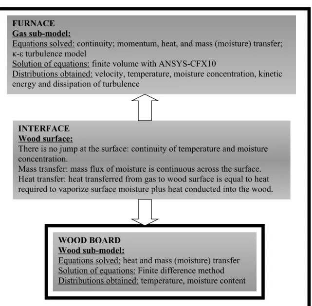
The interface between the two parts is located at the wood surface where the continuity of temperature, moisture concentration as well as heat and mass transfer is ensured.A schematic representation of the mathematical model is given in Figure 1.
The governing equations for the two parts of the system (gas and wood sub-models) are given below.
A total of
23,248 nodes and 124,540 tetrahedral elements on gas side and 64,000 cells on wood side are used. The computation time required for simulating one heat treatment schedule is 8h on Dell Pentium 4 2GHZ CPU and 500 MO of RAM.
Gas:
Continuity Equation
0
V
(1)
Momentum Transfer Equation
( )
) )(
( )
( V V V V
eff f
f P
t
(2)
Heat Transfer Equation
( )
) )(
( )
( c T c T k T
t f pf f pf eff
V
(3)
Mass Transfer Equation (Moisture Concentration)
( )
)
( C D C
t C
eff
V
(4)
Turbulence Model Equations
The effective diffusivity is defined as:
t f
eff
(5)
In the κ-ε model, the turbulent viscosity is calculated from:
t C f 2
(6)
The transport equation for the turbulence kinetic energy (κ) is:
f k
t f f
f P G
t
( V ) ( ) )
(7)
and the turbulence dissipation (ε) is given as:
) (
) ) (
)
( 1 2
f t
f f
f CP C
t
V
(8)
P
κand G are the production of turbulent kinetic energy due to shear and body forces, respectively. The values of the model constants used are
κ=1.0,
=1.4, C
1=1.44, C
2=1.92, C
=0.09. In the regions near the wall where the flow is not fully turbulent, the wall functions are used [21].
Boundary Conditions for the Flow Field
No slip condition is considered on the walls. For the inlets and outlets:
0 /
, 0 /
, 0 /
, 0 /
, 0
, ,
, ,
0 , 0 ,
X X
X C X
T P
Outlet
C C T T w v u u
Inlet in g g in in
(9)
Wood:
Heat Transfer Equation
(k T)
t h
w m
m
(10)
Mass Transfer Equation (Moisture Content)
(D M)
t M
w
(11)
Initial Conditions
T(X, Y, Z,0)=T
0M(X, Y, Z,0)=M
0(12)
Interface between wood and gas at the wood surface:
These are also the heat and mass transfer boundary conditions on the wood surface for the gas and wood sub-models. The temperature and the moisture concentration are continuous across the interface (on the wood surface):
Temperature continuity at the wood-gas interface: T
f= T
s(13)
Concentration continuity at the wood-gas interface: C
f= C(T,M)
s(14)
Heat transfer boundary condition at the wood-gas interface states that the heat transferred from
the gas to the wood surface is equal to the sum of the heat used for the moisture vaporization and
the heat conducted into the wood:
n k T n D C n H
keff T lv eff f f
(15)
Mass transfer boundary condition imposes the continuity of mass flux at the wood-gas interface.
The moisture that diffuses from the interior of the wood to the wood surface should equal to the amount that vaporizes and is removed by the gas:
n D C n
Dw M eff f
w
(16)
Thermo-physical Properties of Birch
The density (ρw) and specific gravity (Gm) of dry birch wood were taken as 480 kg/m3 and 0.48, respectively. Density (ρw), specific heat (cp), and thermal conductivities (kqx, kqy, kqz) of birch containing moisture are determined as a function of temperature and moisture content using relations reported in the literature [11, 22] as given below.
) 100 1
(
*
1000 Gm M
m
(17)
c O
pH p
p c c M M A
c ( 0.01 ) (10.01 )
0 2
(18)
where cpH2O is the heat capacity of water taken as 4.185 J.kg-1.K-1, cp0 is the heat capacity of dry wood, and Ac is a parameter which is a function of moisture content and temperature given as:
T cp0 0.10310.003867 (19)
) 10 . 33 . 1 10
. 36 . 2 06191 . 0
( 4T 4M
M
Ac
(20)
Thermal conductivity as a function of spatial direction and heat of vaporization as a function of T are given by Stanis et al. [23].
01864 . 0 ) 004064 .
0 1941 . 0
(
k G M
kwx wy m (kwx kwy 2kwz) (21)
2
6 160 3.43
10 . 792 .
2 T T
Hlv
(22)
The diffusivity coefficients of wood and gas are calculated using the relation given by Siau [12]:
v bt
v bt
w D D
D D D
) 1 ( )(
1
(
(23)
where
γ is the wood porosity, D
btand D
vare the diffusivities of bound water and vapor, respectively.
D
btand D
vare given as
[12]:
M T
T p
Dv M sat
) 18 . 245 (
) 54 . 1 0 . 1 ( 10 29 .
1 13 1.5
(24)
) 3 . 4 8 . 9 9 . 9
exp( M T
Dbt
(25)
where
φ is the gas relative humidity, and p
satis the vapor pressure at saturation which is
calculated as follows
[12]:
3 6 2 2.44 10 000424
. 0 00759 . 0 74 . 1 exp(
3390 C C C
sat T T T
p
(26)
where T
Cis the critical temperature.
The effective diffusivity of gas is given by Siau [12]:
) 18 . 245 (
10 2 .
9 9 2.5
T T
Deff
(27)
EXPERIMENTAL
The experiments were carried out in the prototype furnace of the University. Pre-dried birch boards were obtained from Scierie Thomas-Louis Tremblay in Ste-Monique, Quebec. Initial wood moisture content was 8-13% (M
0). They were heated under neutral gas atmosphere from room temperature (T
0) to the maximum treatment temperature at a given heating rate. Then, they are kept at that temperature for a predetermined period of time (holding time).
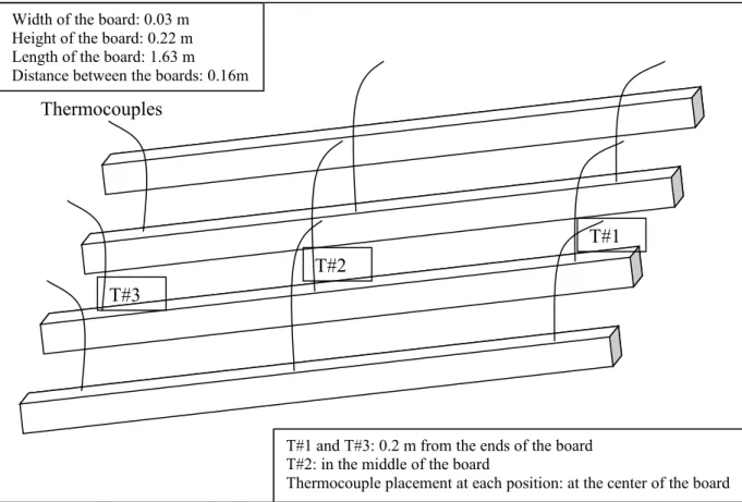
Four birch boards were treated per test. During the tests, the gas and wood temperatures at different positions were followed and recorded. Three thermocouples (two thermocouples, each 20 cm from the ends, and one thermocouple in the middle) were installed in each board, and the thermocouple at each position was placed at the center of the wood board. The dimensions of birch boards as well as the placement of thermocouples are shown in Figure 2.
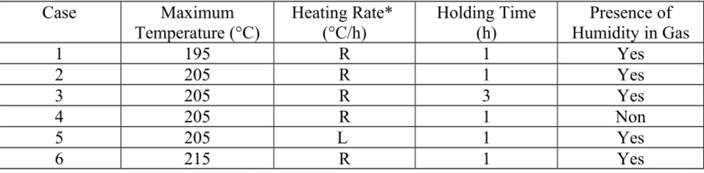
During the tests, the parameters studied are the maximum treatment temperature, heating rate, holding time, and the gas humidity. Table 1 gives the test conditions.
RESULTS AND DISCUSSION
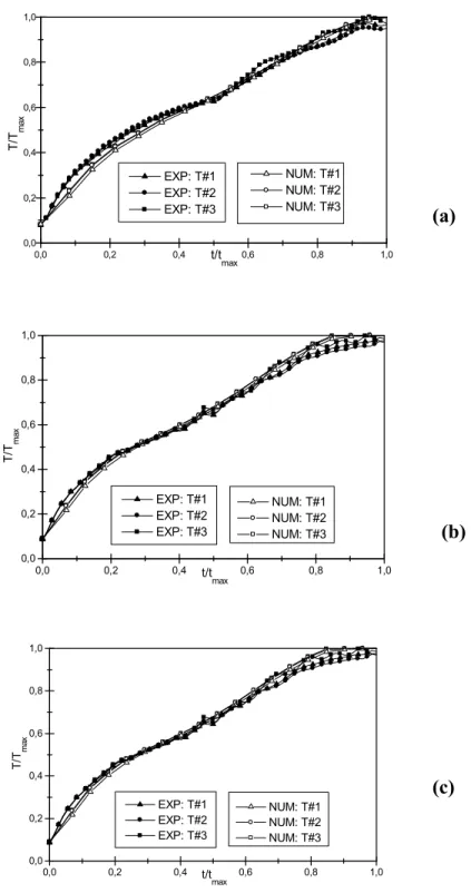
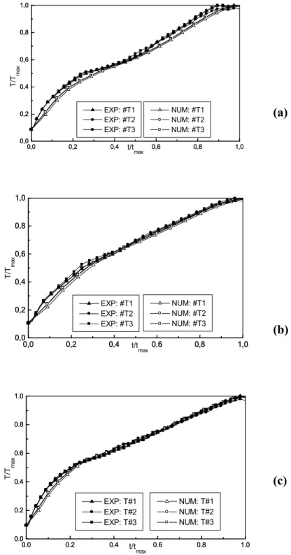
Figures 3 and 4 compare the temperatures measured by three thermocouples (see Figure 2) with
the model predictions under different conditions. Thermocouple readings of all the boards are
similar since the treatment conditions were uniform. As it can be seen from this comparison, model predictions are in good agreement with the experimental results for all the cases considered. The average difference between the model results and the experimental data is in the order of 2-3% depending on the case. The maximum difference is about 3-5% again depending on the case and is observed in the regions where the wood is heated rapidly (t/t
max 0.05 to 0.15).
The differences can be attributed to the discrepancy between the calculated and the actual thermo-physical properties of birch.
The model parameters used for wood constitute the biggest challenge for the model validation.
Wood thermo-physical properties are usually functions of both temperature and moisture content; however, they are not readily available at high temperatures. The model takes into account this dependence. Results indicate that the correlations used represent these properties reasonably well.
The temperature distribution within a wood board at different times is shown in Figure 5(a). In
this figure, X is the direction along the width, Y is the direction along the thickness, and Z is the
direction along the length of the wood board. X
L, Y
L, and Z
Lare the width, thickness, and length
of the wood boards, respectively. As it can be seen from this figure, the temperature profile at
any given time is highly uniform within the wood. There is a small temperature gradient close to
the surface between the surface and the interior of wood on both sides. This gradient decreases
even further with time. The temperature of the gas is higher than that of the surface of the wood
since the wood is heated with a hot gas. Consequently, the surface temperature is slightly higher
than that of the interior. The temperature difference between gas and wood surface makes the
heat transfer from gas to wood possible. If this difference is greater, the wood will not be heated
faster because of its low thermal conductivity. Surface will become a lot hotter than the interior.
This can cause the surface to dry up and develop mechanical stresses. Therefore, the adjustment of gas-wood surface temperature difference is very important for wood heat treatment.
Figure 5(b) presents the normalized moisture content profiles in wood at different times.
Moisture profiles are flat within wood similar to the temperature profiles; however, the moisture gradient close to the surface is steeper compared to that of the temperature gradient. Moisture gradients (gas/wood surface and wood surface/interior of wood) are equally important for the wood heat treatment. As the moisture is transferred from the wood surface to gas, a gradient forms between the interior of wood and the surface. The difference between the gas humidity and wood surface moisture content should be high enough for the moisture removal, but it should not be so large as to cause excessive dryness near the surface. This would result in a large gradient between the surface and interior of wood which consequently would lead to rapid moisture transfer from the interior to the surface and crack formation due to stress. This gradient decreases with time, and after a certain period of time, it is almost flat since the wood surface and gas reach equilibrium.
CONCLUSIONS
The mathematical model developed predicts the experimental results reasonably well. The difference between the model predictions and the measurements can be attributed to wood properties used. Model predictions are found to be in good agreement with the temperatures measured during the heat treatment of birch.
The model also predicts humidity, temperature, and velocity profiles in the gas as well as
temperature and humidity profiles in the wood. Since it has been successfully validated, it can be
used to predict the results of other desired treatments; this, in turn, can reduce the number of experimental trials required for future recipe developments. Model also indicates clearly the uniformity of flow and temperature within the furnace, which is highly important to obtain a good quality product.
ACKNOWLEDGEMENTS
The financial support from Le Fonds québécois de la recherche sur la nature et les technologies (FQRNT), University of Quebec at Chicoutimi (UQAC), Fondation of UQAC (FUQAC), Développement Économique Canada (DEC), Ministère du Développement Économique, de l’Innovation et de l’Exportation (MDEIE), Conférence Régionale des Élus du Saguenay-Lac-St- Jean (CRÉ) and the contributions of Alberta Research Council, Cégep de Saint-Félicien, Forintek, PCI Ind., Ohlin Thermotech, Kisis Technology, and Industries ISA are greatly appreciated.
NOMENCLATURE
Ac
C cp
C, C1, C2
D Pk
h k
M P
=
=
=
=
=
=
=
=
=
constant in cp calculation concentration, kg.m-3 heat capacity, J.kg-1.K-1
constants of κ- turbulence model diffusion coefficient, m2.s-1
shear production of turbulent kinetic energy, m2.s-3
enthalpy, J. kg-1
thermal conductivity, W.m-1.K-1 moisture content, kg H2O.(kg solid)-1 partial pressure of water vapor in wood,
κ σk,
φ γ
Subscripts 0
bt C
=
=
=
=
=
=
=
=
viscous dissipation in turbulent flows, m2s3
turbulent kinetic energy, m2s2 turbulent Prandtl numbers of κ, ε relative humidity, %
wood porosity
initial bound water critical
t T V X, Y, Z XL, YL, ZL
u,v,w Greek
symbols
ΔHlv
=
=
=
=
=
=
=
= Pa time, s temperature, K velocity, m.s-1 spatial coordinates, m dimension of wood boards, m
velocity components in X, Y, and Z directions, m.s-1
density, kg.m-3
dynamic viscosity, kg.m-1.s-1 latent heat of vaporization, J.kg-1
eff f H2O in l m max s sat t v w x, y, z
=
=
=
=
=
=
=
=
=
=
=
=
=
effective fluid water inlet liquid
mixture (wood + moisture) maximum
surface saturation turbulent vapor wood
spatial direction
REFERENCES
[1] Yildiz, S., Building and Environment, 2007, vol. 42, no. 6, pp. 2305-2310.
[2] Rapp, A.O., “Review on Heat Treatments of Wood”, Proceedings of Special Seminar held in Antibes, France, 2001.
[3] Dirol, D., Guyonnet, R., “The Improvement of Wood Durability by Retification Process”, Document No. IRG/WP 98-40015. Int. Research Group on Wood Protection, Stockholm, Sweden, 1993.
[4] Pavlo, B., Niemz, P., Holzforschung, 2003, vol. 57, pp. 539–546.
[5] Kocaefe, D., Shi, J. L., J. Yang, D.Q., Bouazara, M., Forest Product Journal, 2008, vol. 59, no. 6, pp. 88-93.
[6] Stamm, A.J., Ind. and Eng. Chem., 1956, vol. 48, no. 3, pp. 413-417.
[7] Viitaniemi, P., 4
thEurowood Symposium, Stockholm, Sweeden, September 22-23, Tratek, (Swedish Institute for Wood Technology Research), 1997, pp.67-70.
[8] Poncsak, S., Kocaefe, D., Bouazara, M., Pichette, A., Wood Sci. Technol.,2006, vol. 40, pp. 647-668.
[9] Luikov, A.V., Int. J. Heat Mass Transfer, 1975, vol. 18, pp. 1-14.
[10] Luikov, A.V., “Heat and Mass Transfer”, Mir:Moscow, 1980.
[11] Whitaker, S., Adv. Heat Transfer, 1977, vol. 13, pp. 119–203.
[12] Siau, J.F., “Transport Processes in Wood”, Springer-Verlag, New York, 1984.
[13] Bear, J. and Y. Bachmat, “Introduction to Modelling of Transport Phenomena in Porous Media”, Kluwer Academic Publishers, Dordrecht, 1990.
[14] Hassanizadeh, M, Gray, W.G., Adv. Water Res., 1979, vol. 2, pp.131-144.
[15] Younsi, R, Kocaefe, D., Poncsak, S., Kocaefe, Y., International Journal of Energy and Research, 2006a, vol. 30, pp. 699-711.
[16] Younsi, R., Kocaefe, D., Poncsak, S., Kocaefe, Y., Journal of Building Physics, 2006b, vol.
30, no. 2, pp. 113-135.
[17] Younsi, R., Kocaefe, D., Poncsak, S., Kocaefe, Y., AIChE, 2006c, vol. 52, no. 7, pp. 2340- 49.
[18] Osma, A., Kocaefe, D., Kocaefe, Y., Can. J. Chem. Eng.,2008, vol. 86, pp. 693-699.
[19] Younsi, R., Kocaefe, D., Kocaefe, Y., Applied Thermal Engineering, 2007, vol. 27, no. 8- 9, pp. 1424-1431.
[20] Kocaefe, D., Younsi, R., Poncsak, S., Kocaefe, Y., International Journal of Thermal Sciences, 2007, vol. 46, no. 7, pp. 707-716.
[21] Majumdar, P., Deb, P., Numer Heat Transf A, 2003, vol. 43, pp.669–692.
[22] Simpson, W., Tenwold, A., “Physical properties and moisture relations of wood”, in Wood Handbook, USDA Forest service, forest product laboratory, Madison, Wisconsin, U.S., 1999, pp. 1-23.
[23] Stanish M. A,, Schajer G. S., Kayihan, F., 1986, AIChE J, vol. 32, no. 8, pp. 1301–1311.
Figure 1: Schematic Representation of the Mathematical Model FURNACE
Gas sub-model:
Equations solved: continuity; momentum, heat, and mass (moisture) transfer;
κ-ε turbulence model
Solution of equations: finite volume with ANSYS-CFX10
Distributions obtained: velocity, temperature, moisture concentration, kinetic energy and dissipation of turbulence
WOOD BOARD Wood sub-model:
Equations solved: heat and mass (moisture) transfer Solution of equations: Finite difference method Distributions obtained: temperature, moisture content INTERFACE
Wood surface:
There is no jump at the surface: continuity of temperature and moisture concentration.
Mass transfer: mass flux of moisture is continuous across the surface.
Heat transfer: heat transferred from gas to wood surface is equal to heat
required to vaporize surface moisture plus heat conducted into the wood.
Figure 2: Placement of Boards and Thermocouples in the Furnace
T#1 and T#3: 0.2 m from the ends of the board T#2: in the middle of the board
Thermocouple placement at each position: at the center of the board
Thermocouples
T#1 T#2
T#3
Width of the board: 0.03 m Height of the board: 0.22 m Length of the board: 1.63 m Distance between the boards: 0.16m
B 0,0
0,2 0,4 0,6 0,8 1,0
EXP: T#1 EXP: T#2 EXP: T#3
0,0 0,2 0,4 0,6 0,8 1,0
B
NUM: T#1 NUM: T#2 NUM: T#3 T/T max
t/tmax
B 0,0
0,2 0,4 0,6 0,8 1,0
NUM: T#1 NUM: T#2 NUM: T#3 T/T max
t/tmax
0,0 0,2 0,4 0,6 0,8 1,0
B
EXP: T#1 EXP: T#2 EXP: T#3
B 0,0
0,2 0,4 0,6 0,8 1,0
NUM: T#1 NUM: T#2 NUM: T#3 T/T max
t/tmax
0,0 0,2 0,4 0,6 0,8 1,0
B
EXP: T#1 EXP: T#2 EXP: T#3
Figure 3: Comparison of Model Predictions with Experimental Measurements for Thermocouples 1, 2, and 3 at Different Maximum Treatment Temperatures for (a) Case 1, (b)
Case 2, and (c) Case 6 (see Table 1)
(a)
(b)
(c)
0,0 0,2 0,4 0,6 0,8 1,0 0,0
0,2 0,4 0,6 0,8 1,0
NUM: #T1 NUM: #T2 NUM: #T3 t/tmax
0,0 0,2 0,4 0,6 0,8 1,0
0,0 0,2 0,4 0,6 0,8 1,0
EXP: #T1 EXP: #T2 EXP: #T3 T/Tmax
0,0 0,2 0,4 0,6 0,8 1,0
0,0 0,2 0,4 0,6 0,8 1,0
NUM: #T1 NUM: #T2 NUM: #T3 t/tmax
0,0 0,2 0,4 0,6 0,8 1,0
0,0 0,2 0,4 0,6 0,8 1,0
EXP: #T1 EXP: #T2 EXP: #T3 T/T max
0.0 0.2 0.4 0.6 0.8 1.0
0.0 0.2 0.4 0.6 0.8 1.0
NUM: T#1 NUM: T#2 NUM: T#3 t/tmax
0.0 0.2 0.4 0.6 0.8 1.0
0.0 0.2 0.4 0.6 0.8 1.0
EXP: T#1 EXP: T#2 EXP: T#3 T/T max
Figure 4: Comparison of Model Predictions with Experimental Measurements for
Thermocouples 1, 2, and 3 Under Different Conditions for (a) Case 3, (b) Case 4, and (c) Case 5 (see Table 1)
(a)
(b)
(c)
0,0 0,2 0,4 0,6 0,8 1,0 0,0
0,2 0,4 0,6 0,8 1,0
t/tmax=0.06 t/tmax=0.53 t/tmax=0.76
t/tmax=0.88 t/tmax=1.0
T /T
maxX/X
L0,0 0,2 0,4 0,6 0,8 1,0
0,0 0,2 0,4 0,6 0,8 1,0
t/tmax=1.0 t/tmax=0.88 t/tmax0.76 t/tmax=0.53 t/tmax=0.06