From monsoon to marine productivity in the Arabian Sea: insights from glacial and interglacial climates

HAL Id: hal-01584174

https://hal.archives-ouvertes.fr/hal-01584174

Submitted on 3 Nov 2017

HAL is a multi-disciplinary open access

archive for the deposit and dissemination of

sci-entific research documents, whether they are

pub-lished or not. The documents may come from

teaching and research institutions in France or

abroad, or from public or private research centers.

L’archive ouverte pluridisciplinaire HAL, est

destinée au dépôt et à la diffusion de documents

scientifiques de niveau recherche, publiés ou non,

émanant des établissements d’enseignement et de

recherche français ou étrangers, des laboratoires

publics ou privés.

Sea: insights from glacial and interglacial climates

Priscilla Le Mézo, Luc Beaufort, Laurent Bopp, Pascale Braconnot, Masa

Kageyama

To cite this version:

Priscilla Le Mézo, Luc Beaufort, Laurent Bopp, Pascale Braconnot, Masa Kageyama. From monsoon

to marine productivity in the Arabian Sea: insights from glacial and interglacial climates. Climate

of the Past, European Geosciences Union (EGU), 2017, 13 (7), pp.759-778. �10.5194/cp-13-759-2017�.

�hal-01584174�

https://doi.org/10.5194/cp-13-759-2017

© Author(s) 2017. This work is distributed under the Creative Commons Attribution 3.0 License.

From monsoon to marine productivity in the Arabian Sea:

insights from glacial and interglacial climates

Priscilla Le Mézo1, Luc Beaufort2, Laurent Bopp1, Pascale Braconnot1, and Masa Kageyama1

1_{LSCE/IPSL, UMR 8112, CEA/CNRS/UVSQ, Centre CEA-Saclay, Orme des Merisiers, 91191 Gif-sur-Yvette, France}

2_{CEREGE, UMR 7330, CNRS-IRD-Aix Marseille Université, Av. Louis Philibert, BP80, 13545 Aix-en-Provence, France}

Correspondence to:Priscilla Le Mézo (priscilla.le-mezo@lsce.ipsl.fr) Received: 29 August 2016 – Discussion started: 13 September 2016

Revised: 31 March 2017 – Accepted: 14 April 2017 – Published: 4 July 2017

Abstract. The current-climate Indian monsoon is known to boost biological productivity in the Arabian Sea. This paradigm has been extensively used to reconstruct past mon-soon variability from palaeo-proxies indicative of changes in surface productivity. Here, we test this paradigm by simu-lating changes in marine primary productivity for eight con-trasted climates from the last glacial–interglacial cycle. We show that there is no straightforward correlation between bo-real summer productivity of the Arabian Sea and summer monsoon strength across the different simulated climates. Locally, productivity is fuelled by nutrient supply driven by Ekman dynamics. Upward transport of nutrients is mod-ulated by a combination of alongshore wind stress inten-sity, which drives coastal upwelling, and by a positive wind stress curl to the west of the jet axis resulting in upward Ekman pumping. To the east of the jet axis there is how-ever a strong downward Ekman pumping due to a negative wind stress curl. Consequently, changes in coastal along-shore stress and/or curl depend on both the jet intensity and position. The jet position is constrained by the Indian sum-mer monsoon pattern, which in turn is influenced by the as-tronomical parameters and the ice sheet cover. The astro-nomical parameters are indeed shown to impact wind stress intensity in the Arabian Sea through large-scale changes in the meridional gradient of upper-tropospheric temperature. However, both the astronomical parameters and the ice sheets affect the pattern of wind stress curl through the position of the sea level depression barycentre over the monsoon region

(20–150◦W, 30◦S–60◦N). The combined changes in

mon-soon intensity and pattern lead to some higher glacial pro-ductivity during the summer season, in agreement with some palaeo-productivity reconstructions.

1 Introduction

The Arabian Sea biological productivity is influenced by the strong seasonal activity of the atmospheric circulation (Creary et al., 2009; Ivanova et al., 2003; Schott and Mc-Creary, 2001; Lee et al., 2000; Luther et al., 1990). Dur-ing the boreal summer, the south-west monsoon consists of strong winds blowing from the south-west to the north-east of the Indian Ocean. These winds result from the rapid heating of the land mass relative to the ocean, which cre-ates a pressure gradient between the southern Indian Ocean high-pressure cell and the low-pressure cell over the Tibetan Plateau. During this season, heavy precipitation occurs over India and south-east Asia. In the Arabian Sea, the along-shore winds off the coast of Somalia focus into a low-level jet, called the Somali Jet, and generate a strong coastal up-welling (Anderson et al., 1992; Findlater, 1969). In addi-tion, the wind’s tendency to turn on itself in the horizon-tal plane, quantified by the wind stress curl, also drives up-ward and downup-ward water transport (Marshall and Plumb, 2008). Between the axis of the jet and the western coast, the wind stress is cyclonic and the wind stress curl is pos-itive; it drives a divergent flow that causes upward Ekman pumping (Murtugudde et al., 2007; Barber et al., 2001; An-derson et al., 1992; Findlater, 1969). On the other side of the jet axis, however, the wind stress is anticyclonic. The wind stress curl is therefore negative and drives a conver-gent flow and downward Ekman pumping. Coastal upwelling and upward Ekman pumping are responsible for increased productivity in the western coastal Arabian Sea thanks to a higher supply of nutrients to the surface layer (Anderson et al., 1992; Anderson and Prell, 1992). The upwelled

nutri-ents are advected from the coast to the north and the inte-rior of the sea. Thus, productivity in the central and northern Arabian Sea also increases during the south-west monsoon (Caley et al., 2011; Prasanna Kumar et al., 2001; Keen et al., 1997). Wind stress and mixing of the upper layers, as well as Ekman pumping generated by the positive wind stress curl, also contribute to the supply of nutrients to the surface lay-ers and increase productivity in those regions (Wiggert et al., 2005; Prasanna Kumar et al., 2001; Lee et al., 2000). On the mesoscale, filaments contribute to the lateral advection of nu-trients from the coast to the central Arabian Sea (Resplandy et al., 2011).

Monsoon intensity can be characterised in different ways, depending on the observational scale and on the studied processes. Precipitation is a major indicator of monsoonal changes. For example, the rainfall-based index, defined as the seasonally averaged precipitation over all the Indian subcon-tinent from July to September, is used to monitor the strength of the monsoon over India (Mooley and Parthasarathy, 1984). However, Held and Soden (2006) indicate that, in the context of anthropogenic climate change, an increase in rainfall is not necessarily associated with an increase in the associated circulation due to changes in atmospheric stability. This re-sult questions the reliability of such an indicator for the mon-soon intensity. A second indicator of the monmon-soon strength is based on the sea level pressure (SLP) that is a large-scale fin-gerprint of the monsoon. The monsoon strength can be de-termined by the SLP anomaly gradient between a northern region over the Tibetan Plateau, where the Tibetan low devel-ops during the monsoon months, and a southern region over the southern Indian Ocean, where the Mascarene High devel-ops. The large-scale changes in SLP impact the local dynam-ics over the Arabian Sea (Schott and McCreary, 2001). Mon-soon intensity can also be related to the strength of the winds over the Arabian Sea and the associated upwelling. The gen-eral paradigm is that a stronger summer monsoon generates stronger upwelling that enhances productivity. Based on this paradigm, past monsoon intensities have been reconstructed using proxies of productivity from marine sediment cores (Caley et al., 2011; Ivanova et al., 2003; Clemens and Prell, 2003).

Monsoon reconstructions and modelling studies (Marzin and Braconnot, 2009; Braconnot et al., 2008; Anderson and Prell, 1992; Prell et al., 1992) have shown that insolation variations are the major drivers of fluctuations in the sum-mer monsoon intensity: the monsoon is stronger when the Northern Hemisphere summer insolation is higher (e.g. dur-ing the Holocene). Changes in the astronomical parameters, such as the precession that is defined as the longitude of the perihelion, or the obliquity that is defined as the angle between the Equator and the orbital plane, modify the sea-sonal cycle of insolation. Along with astronomical param-eters, changes in ice sheet height between glacial and terglacial climates also have an impact on the monsoon

in-tensity (Masson et al., 2000; Emeis et al., 1995; Prell et al., 1992; Anderson et al., 1992).

There has been some concern about the fact that ma-rine proxies for productivity may be influenced by processes other than monsoon intensity, such as changes in ice volume, especially in the Northern Hemisphere; aeolian transport of nutrients; or the Atlantic Meridional Overturning Circulation (Ruddiman, 2006; Ziegler et al., 2010; Caley et al., 2011). Moreover, most studies linking monsoon and productivity in the past have focused on the monsoon intensity but the mon-soon pattern, e.g wind orientation, can also change in time. Sirocko et al. (1991) have shown that summer monsoon mean position shifted southward during glacial periods. The mon-soon pattern affects the position and the orientation of the low-level jet over the Arabian Sea, which modifies the up-welling of nutrients in the Arabian Sea (Anderson and Prell, 1992). Furthermore, Bassinot et al. (2011) showed opposite evolutions of the upwelling behaviour in the western coastal Arabian Sea and the south-western tip of India during the Holocene, which they related to a southward shift of the mon-soonal winds.

Here, we investigate the relationship between the sum-mer monsoon intensity and the Arabian Sea biological pro-ductivity. How do changes in the summer monsoon pattern along with changes in its intensity impact productivity in the Arabian Sea? Could the variations in the summer mon-soon pattern explain higher productivity rates in some glacial climates? To answer these questions, we test the effects of a range of astronomical parameters and different ice sheet states on the Arabian Sea productivity.

In Sect. 2, we describe the model we use and the exper-iments we performed, we evaluate the model results for the pre-industrial period and detail the analyses we performed. In Sect. 3, we explain the changes in productivity in the early Holocene and then look at several glacial and interglacial climates to link productivity changes to local dynamics and boundary conditions. In Sect. 4, we discuss our results in the light of the summer monsoon paradigm and we perform a simple model–data comparison and discuss the effects of sea-sonality on productivity. Finally, we summarise our results and give some perspectives.

2 Model, experiments, evaluation and diagnostics

2.1 The model

This study uses an Earth system model (ESM) that explicitly represents the global climate, oceanic circulation and marine productivity. We use the IPSL-CM5A-LR model developed at the Institut Pierre Simon Laplace (IPSL) (Dufresne et al., 2013). This ESM is composed of the LMDZ5A atmospheric general circulation model (Hourdin et al., 2013) coupled to the ORCHIDEE land-surface model (Krinner et al., 2005) and the NEMO v3.2 ocean model (Madec, 2011), which in-cludes the OPA9 ocean general circulation model, LIM-2

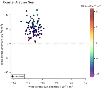
Table 1.Boundary conditions for the eight simulations studied in this work. Precession is defined as the longitude of the perihelion, relative to the moving vernal equinox, minus 180◦. Ice sheets are represented in Fig. 1. Pmip3 ice sheet stands for the PMIP3 ice sheet reconstruction (Abe-Ouchi et al., 2015), ICE6g-16k stands for the ICE6G reconstruction at 16 kyr BP (Peltier et al., 2015).

Interglacial climates Glacial climates

Simulation name CTRL MH EH LGM MIS3 MIS4F MIS4M MIS4D

Time (kyr BP) 0 6 9.5 21 46 60 66 72

Ice sheets present present present pmip3 Ice6g-16k Ice6g-16k Ice6g-16k Ice6g-16k

Sea level difference vs. CTRL (m) 0 0 0 −120 −70 −70 −70 −70

Eccentricity 0.016715 0.018682 0.0193553 0.018994 0.0138427 0.018469 0.021311 0.024345 Obliquity (◦) 22.391 24.105 24.2306 22.949 24.3548 23.2329 22.493 22.391 Precession (ω − 180◦) 102.7 0.87 303.032 114.42 101.337 266.65 174.82 80.09 CO₂(ppm) 284 280 284 185 205 200 195 230 N₂O (ppm) 275 270 275 200 260 230 217 230 CH₄(ppb) 791 650 791 350 500 426 450 450

the sea-ice component (Fichefet and Maqueda, 1997) and the PISCES biogeochemical model (Aumont and Bopp, 2006). These components are coupled once a day using the OASIS coupler (Valcke, 2012).

We use the low-resolution (LR) version of the model with a regular atmospheric grid of 96 × 96 points horizontally, 39 vertical levels and an irregular horizontal oceanic grid (ORCA2.0) with 182 × 149 points corresponding to a

nom-inal resolution of 2◦, enhanced near the Equator and over

the Arctic and subpolar North Atlantic. The ocean vertical grid comprises 31 levels with intervals from 10 m for the first 150 m and up to 500 m for the bottom of the ocean.

The PISCES model simulates marine biogeochemistry and lower trophic levels. PISCES includes two phytoplankton types (nanophytoplankton and diatoms), two zooplankton size classes (micro- and mesozooplankton) and two detritus compartments distinguished by their vertical sinking speed (small and large organic matter particles), a semi-labile dis-solved organic carbon pool, and five nutrients (Fe, NO−₃, NH+₄, Si, and PO3−₄ ) (Aumont and Bopp, 2006). In PISCES, phytoplankton growth is a function of temperature, light, mixed-layer depth and nutrient concentrations.

2.2 Experiments

Here, we exploit eight simulations of IPSL-CM5A-LR forced by different boundary conditions (astronomical pa-rameters, greenhouse gas concentrations and ice sheet cover) to account for different climates throughout the last glacial– interglacial cycle, as detailed in Table 1 and Fig. 1.

The reference (CTRL) simulation is a pre-industrial cli-mate with no external forcing such as volcanoes or anthro-pogenic activities (Dufresne et al., 2013), forced by pre-industrial CMIP5 forcings (Taylor et al., 2012) and the present-day ice sheet (0k in Fig. 1). A mid-Holocene (MH) simulation, 6 kyr BP (Kageyama et al., 2013), part of Paleo-climate Modeling Intercomparison Project phase 3 (PMIP3) (Braconnot et al., 2012) and an early Holocene (EH)

sim-ulation, 9.5 kyr BP, are used to study productivity changes in different interglacial climates. The EH simulation trace gas concentrations are the same as for the CTRL simula-tion, whereas CH4and N2O concentrations are slightly lower for the MH simulation compared with the CTRL (Table 1). MH and EH simulations mainly differ in their astronomi-cal parameters, especially in the precession value (Table 1, Fig. 1). Both Holocene simulations are forced by the present-day ice sheet cover (Fig. 1). Five glacial simulations have also been performed, including the last glacial maximum (LGM, 21 kyr BP), the marine isotopic stage 3 (MIS3, 46 kyr BP) and three marine isotopic stage 4 states: MIS4F (60 kyr BP), MIS4M (66 kyr BP) and MIS4D (72 kyr BP). The LGM, which has also been performed for PMIP3 (Kageyama et al., 2013), has the largest ice sheet (Fig. 1) (Abe-Ouchi et al., 2015), which modifies the land–sea distribution and topogra-phy since the sea-level is reduced by about 120 m. The LGM run has the lowest greenhouse gas concentrations of this set of eight simulations (Table 1). Two of the three MIS4 simu-lations (MIS4F and MIS4D) are described in Woillez et al. (2014). The MIS4 ice sheets have been prescribed by us-ing the 16 kyr BP ice sheet, which is the period for which we have an ice sheet reconstruction for the same sea level as during MIS4, i.e. 70 m lower than today (Ice6g-16k in Fig. 1) (Peltier et al., 2015). This is the most realistic sce-nario we could simulate given the available reconstruction at the time of running the MIS4 experiments (Woillez et al., 2014). However, our MIS4 runs are different from the ones described in Woillez et al. (2014) since we added the nutri-ent inputs from dust, rivers and sedimnutri-ents that are essnutri-ential to marine productivity. Large changes in precession occur between the three MIS4 simulations (Table 1, Fig. 1). The MIS3 simulation uses the same ice sheet reconstruction as MIS4 and it has the lowest eccentricity and highest obliquity of all eight simulations (Table 1, Fig. 1).

In PISCES, three source terms contribute to the input of nutrients in the ocean: atmospheric dust deposition, river in-put and sediment mobilisation. The change in sea level in

(a) ( b) 0.0138 0.0167 0.0185 0.0213 0.0243 0.87 80.09114.42 174.82 266.65 360 22.391 22.949 23.446 24.105 185195200205 230 280284 200 217 230 260 270 275 xn yn Eccentricity (°) Obliquity (°) Precession (w-180°) CO2 (ppm) CH4 (ppm) N2O (ppb) 350 426450500 650 791 CTRL MH EH LGM MIS3 MIS4F MIS4M MIS4D Present pmip3 ice6g-16k

Figure 1.(a) The three ice sheet covers used as boundary conditions. The 0k ice sheet is used in the CTRL, MH and EH simulations. The pmip3 ice sheet (Abe-Ouchi et al., 2015) is used in the LGM simulation. The ICE6g-16k ice sheet (Peltier et al., 2015) is used in the MIS3 and all the MIS4 (F, M and D) simulations and (b) the different values of the other forcing parameters for all the simulations.

glacial climate simulations modifies the land–sea mask; thus, in the LGM, MIS3 and all MIS4 (F, M and D) simulations, the source terms were adjusted so that the ocean receives the same quantity of associated nutrient supply as in the CTRL. In these simulations, no attempt was made to account for the dustier glacial states (Bopp et al., 2003). All productivity changes are therefore due to other factors.

Our analyses are performed on 100 years of monthly out-puts from the last stable part of each simulation.

2.3 Modern evaluation of the summer mean

This study focuses on primary productivity in the Indian Ocean for the last glacial–interglacial cycle as simulated by the IPSL-CM5A-LR coupled model. Figure 2 shows the sea-sonal cycle of observed present-day productivity (data from SeaWiFS 1998–2014; Lévy et al., 2007) for two areas in the Arabian Sea: a coastal area in the western Arabian Sea (Fig. 2a, orange area) and a northern region (Fig. 2a, black box). Current-day productivity has two periods of bloom: one in summer and one in winter. In the coastal Arabian Sea, the summer season is the most productive period of the year (Fig. 2b) and contributes the most to the bulk sed-iment composition. In the northern Arabian Sea, both sea-sons are equally productive in the data (Fig. 2b). In boreal

winter, the mechanisms behind productivity peaks are differ-ent compared with the summer maximum; the winds reverse and blow from the north-east to the south-west. The presence of strong southward winds generates a convective overturn-ing that induces vertical mixoverturn-ing and broverturn-ings nutrients to the surface. During this period, productivity is high in the north-western Arabian Sea (dashed line in Fig. 2b). Following these observations, we focus our analyses on the boreal summer season, defined as June–July–August–September (JJAS) to account for the whole summer monsoon, and we will es-pecially analyse the coastal Arabian Sea (orange area in Fig. 2a).

A comparative global evaluation of the marine bio-geochemical component of the ESM has been published in Séférian et al. (2013). Even if the model poorly represents the deep-ocean circulation, especially in the Southern Ocean, it has a quite good representation of annual wind patterns, wind stress, mixed-layer depth and geostrophic circulation. The model is able to represent the global ocean biologi-cal fields such as macronutrients, with correlations higher than 0.9, and surface chlorophyll concentration, with a cor-relation coefficient of 0.42 (Séférian et al., 2013). We focus here on the representation of the physical processes and pro-ductivity distributions in the Indian Ocean, especially in the Arabian Sea. We use satellite products from remote sensing

(a) Regions of interest (b) Satellite-based productivity Time (month) PP (molC m -2 yr -1)

Jan Feb Apr Jun Jul Aug Oct Dec 20

40 60 80

Mar May Sep Nov

Coastal AS Northern AS

Core MD04-2873

Figure 2.(a) Coastal (orange shading) and northern (black dotted contour) Arabian Sea areas, position of core MD04-2873 (yellow circle) and (b) seasonal cycles of current-day productivity in the coastal (bold orange line) and northern (black dashed line) Arabian Sea. Productivity data come from the SeaWiFS satellite data for the period 1998–2005 (Lévy et al., 2007).

from NASA’s Sea-viewing Field-of-view Sensor (SeaWiFS) during the period 1998–2005 processed with the algorithm (Behrenfeld and Falkowski, 1997) to obtain monthly produc-tivity (Lévy et al., 2007), multiple-satellite products from NOAA for the 1995–2005 climatological cycle for wind in-tensity and wind stress (Zhang, 2006) and the ERA-Interim reanalysis (1979–2014) for sea surface temperature (SST) (Dee et al., 2011). We compute the observed and modelled wind stress curl intensity from the wind stress data and model output, respectively. We compare the observations to the pre-industrial (CTRL) simulation outputs.

Figure 3a shows that simulated boreal summer produc-tivity integrated over the whole water column is underesti-mated relative to the reconstructed boreal summer produc-tivity, especially in the regions of upwelling, along the coast of the Arabian Peninsula and Somalia. The spatial Pear-son’s correlation coefficient, R, between the observed and simulated productivity is 0.44. Underestimation of produc-tivity is first caused by an underestimated wind intensity (Fig. 3b), which affects the extent and intensity of the coastal upwelling and the supply of nutrients to the surface layer. The boreal summer wind patterns, which are characteristic of the boreal summer monsoon system, are better represented than productivity, with a correlation of 0.86. Sperber et al. (2013) studied the representation of the Asian summer mon-soon in the CMIP5 models, which comprise the IPSL model. They showed that the monsoon was better represented in the CMIP5 models compared with the CMIP3 models, es-pecially the monsoonal winds. We can however note that the alongshore winds in the western Arabian Sea have a more northerly orientation in the CTRL simulation than in the ob-servations, which can affect the dynamical processes in the region (Fig. 3b).

In the Arabian Sea, summer productivity is affected by the winds through different mechanisms driven by the wind stress and the wind stress curl (Anderson et al., 1992). The strong winds along the Arabian coast, called the Somali Jet,

generate a positive wind stress, which increases Ekman trans-port off the coast. The water that leaves the coastal area is replaced by subsurface water: this is the coastal upwelling. Similar to the wind intensity, the CTRL simulation wind stress intensity is underestimated compared with the reanal-yses: the maximum wind stress intensity is lower and it does not extend as far north in the Arabian Sea as the reconstructed wind stress (Fig. 3c). The wind stress orientation is also more zonal in the simulation than in the observations, which causes the simulated wind stress to be higher close to the Oman coast relative to the observations (Fig. 3b, c). Figure 3d rep-resents the wind stress curl, computed from the wind stress, in the simulation and in the observations. The simulated dis-tribution resembles the reconstructed one: on the left-hand side of the strong low-level wind jet, between the coast and the maximum wind intensity, the curl in the wind stress is positive and on the other side of the jet the wind stress curl is negative. The differences seen in the jet position and width are transmitted to the wind stress and wind stress curl inten-sity and distribution, with an overall less positive curl close to the coast and less negative curl offshore in the simulation. In Fig. 3e, we can see that the modelled SST anomalies, relative to the global averaged SST in boreal summer, are underesti-mated in the Arabian Sea, especially close to the Oman coast, suggesting a less intense upwelling activity compared with the observations. This is coherent with the underestimated wind stress and wind stress curl intensities, which control the upward Ekman pumping intensity (Fig. 3c, d).

Discrepancies between our pre-industrial simulation and the observations may be due to the coarse model resolu-tion. In Resplandy et al. (2011), a higher-resolution version of the model was used to study the effects of mesoscale dy-namics on productivity. They showed that the model is able to reproduce the observed mesoscale dynamics, such as the Great Whirl and filaments that transport nutrients from the coast to the open sea. They highlighted the major role of the eddy-driven transports in the establishment of biological

°

Figure 3.Modelled and observed seasonal (JJAS) patterns of (a) productivity (molC m−2yr−1), (b) surface wind intensity (m s−1), (c) sur-face wind stress intensity (10−3N m−2), (d) surface wind stress curl intensity (10−7N m−3) and (e) sea surface temperature (SST) (◦C). We used SeaWiFS data in 1998–2005 for productivity (Lévy et al., 2007), multiple-satellite products from NOAA 1995–2005 (Zhang, 2006) for the climatology of surface wind, wind stress and wind stress curl intensity and the ERA-Interim reanalysis 1979–2014 for SST (Dee et al., 2011).

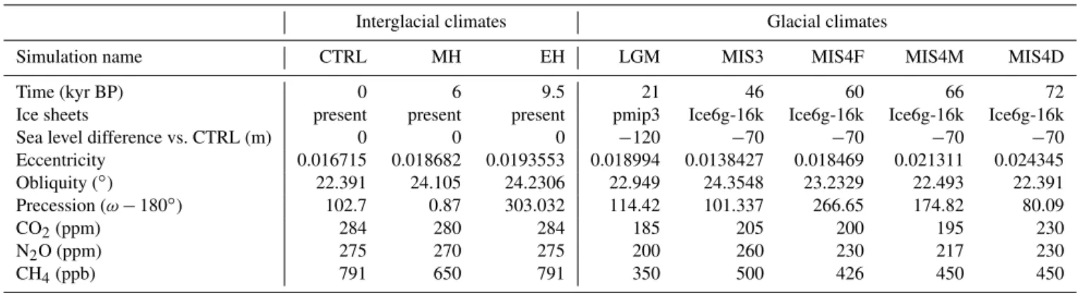
blooms in the Arabian Sea and the model’s ability to repre-sent the different physical processes at stake behind produc-tivity blooms in summer and in winter in the region. Nev-ertheless, even though both the winds and productivity are underestimated in CTRL by the lower-resolution version of the model, the physical mechanisms playing a role in the marine productivity are represented, which therefore makes the simulations suitable for our study. Figure 4 illustrates the combined effects of wind stress and wind stress curl on pro-ductivity in the coastal Arabian Sea (orange area in Fig. 2a) on the inter-annual timescale. It shows that if the summer (JJAS) wind stress and wind stress curl intensities are higher than their summer average, productivity is higher than av-erage in the coastal Arabian Sea (upper-right quadrant). It also highlights that the higher the wind stress and the wind stress curl anomalies, the higher the productivity change, and conversely. This is coherent with the fact that both the wind stress and the wind stress curl act to bring nutrient-rich wa-ters to the surface and fuel productivity in boreal summer

(Anderson et al., 1992; Murtugudde et al., 2007). Figure 4 also shows that a high wind stress curl (wind stress) can compensate a reduced wind stress (wind stress curl) intensity and lead to higher-than-average productivity (lower-right and upper-left quadrants in Fig. 4, respectively).

2.4 Diagnostics

In this section we briefly describe the variables and the methods we use throughout the paper. We are interested in the links between the large-scale Indian summer mon-soon system and the Arabian Sea primary productivity. To characterise the boreal summer monsoon intensity, we use the meridional gradient of upper-tropospheric tem-perature (TT, averaged from 200 to 500 hPa) between a northern region covering India, south-east Asia, the

Ti-betan Plateau (60–120◦E, 10–45◦N) and a southern

re-gion over the tropical Indian Ocean (60–120◦E, 25◦S–

−1.5 −1.0 0.5 1.0 −40 −20 0 20 40 JJAS mean : TPP = 28.3 mol C m-2 _yr-1 Stress = 143.3 x 10-3 _{N m}-2 Curl = 0.5 x 10-7 _{N m}-3 TPP (mol C m-2 yr-1) CTRL simulation, JJAS, coastal Arabian Sea

−0.5 0.0

Wind stress curl (10-7 _{N m}-3₎

Wind stress (10 -3 N m -2) ● ● ● ● ● ● ● ● ● ● ● ●● ● ● ● ● ● ● ● ● ● ● ● ● ● ● ● ● ● ● ●_● ● ● ● ● ● ● ● ● ● ● ● ● ● ● ● ● ● ● ● ● ● ● ● ● ● ● ● ● ● ● ● ● ● ● ● ● ● ● ● ● ● ● ●_● ● ● ● ● ● ● ● ● ● ● ● ● ● ● ● ● ● ●● ● ● ● ● −10 −5 0 5 10

Figure 4. Anomalies of total primary productivity (TPP, molC m−2yr−1, represented by the colour scale) integrated over the whole water column as a function of wind stress anomalies (10−3N m−2, y axis) and wind stress curl anomalies (10−7N m−3, x axis) in the western coastal Arabian Sea (see Fig. 2a) for the CTRL simulation. Anomalies are computed as the difference be-tween each summer average (JJAS) and the seasonal summer mean of the corresponding variable in the CTRL simulation. The colour of the circles represents the value of the change in TPP compared with the CTRL. The colour scale, x axis range and y axis range are the same as those in Figs. 7 and 10.

This gradient, 1TT, is associated with the land–sea contrast in temperature (Marzin and Braconnot, 2009). 1TT is aver-aged over the boreal summer period (JJAS) and the higher its value, the stronger the Indian summer monsoon.

Changes in the monsoon intensity and pattern affect the SLP field. We compute the SLP from the model outputs (i.e. model air temperature and pressure, within and between the atmospheric grid levels, and orography) using the extrapola-tion described in Yessad (2016). We define SLP anomalies as the SLP minus the global annual average of SLP. In order to characterise the monsoon pattern, we compute the barycentre of the region defined by an SLP anomaly lower than −5 hPa over the region covering the African, east Asian and Indian monsoon regions of influence (20◦W–150◦E, 30◦S–60◦N) and we call SLPa-5 the region delimited by the −5 hPa con-tour in SLP anomalies (Fig. 5c–f). This SLPa-5 barycentre is representative of the balance between the different mon-soons as well as of the Indian summer monsoon wind po-sition and direction over the Arabian Sea. A modification of the monsoon pattern, which can have impacts on productivity through atmospheric forcing onto the ocean circulation, can then be related to movements of the SLPa-5 barycentre. We only focus on the Tibetan low since the Mascarene High, the region of high SLP in the southern Indian Ocean, barycentre remains quite similar in the different simulations.

Anderson et al. (1992) showed that the wind stress inten-sity generates coastal upwelling and that the positive wind stress curl is responsible for upward Ekman pumping off-shore. We focus our work on these two wind variables in the coastal western Arabian Sea, a region of positive curl, for the CTRL climate, between the axis of the Somali Jet and the coast (Fig. 2a, orange area).

In the following sections of the paper, total primary pro-ductivity (TPP) is defined as the sum of nanophytoplankton and diatoms total net primary productivity integrated over the whole water column. We also analyse nitrate concentrations in the first 30 m of the water column, nitrate being the ma-jor limiting nutrient in the region, and its supply to the sur-face layers being mainly driven by atmospheric changes via coastal upwelling and upward Ekman pumping.

We use the CTRL simulation as a reference. All changes are then defined relative to this pre-industrial simulation.

3 Simulated palaeo-productivity and monsoon changes

In this section, we investigate the changes in summer produc-tivity in past climate simulations with respect to the CTRL simulation, starting with the early Holocene and then gener-alising to all the climates.

3.1 The early Holocene case

The EH experiences a stronger Indian summer monsoon than the pre-industrial period (Fig. 5). Therefore, we would ex-pect higher productivity in the Arabian Sea. However, the EH simulation shows lower levels of productivity than in the CTRL (Fig. 6). We explain this counter-intuitive result by a change in the monsoon pattern instead of a change in its in-tensity (Fig. 7).

The early Holocene, which we choose to represent with a snapshot at 9.5 kyr BP, is an interglacial period that mainly differs from the pre-industrial period because of the imposed obliquity (24.2306◦ vs. 22.391◦) and precession (303.032◦

vs. 102.7◦) (Table 1). These changes in astronomical

pa-rameters cause the boreal summer insolation in the North-ern Hemisphere to be higher than in the pre-industrial cli-mate (Marzin and Braconnot, 2009). In our simulation of EH, the boreal summer (JJAS) Northern Hemisphere (0–

90◦N, NH) mean insolation is 20 W m−2higher than in the

CTRL (Fig. 5a, b). This change in insolation modifies the upper-tropospheric temperature gradient, 1TT, represented in Fig. 5c, d: in EH, 1TT is 1 K higher than in CTRL, sup-porting a stronger monsoon intensity consistent with previ-ous studies (Marzin and Braconnot, 2009; Goswami et al., 2006).

The large-scale spatial pattern of the summer monsoon is also different in EH compared with CTRL. Maps (e) and (f) in Fig. 5 show the SLP anomalies and the location of the SLPa-5 barycentre. The EH depression extends further to the

Figure 5.(a, b) Seasonal cycle of the insolation at the top of the atmosphere (W m−2) in (a) the CTRL simulation and (b) the difference between EH and CTRL. The Northern Hemisphere (0–90◦N) mean summer (JJAS) insolation, NHmean(JJAS), in CTRL and the difference

between the EH and CTRL simulations, 1NHmean(JJAS), is given under panels (a, b), respectively. (c, d) Upper-tropospheric temperature

(TT) averaged between 200 and 500 hPa in (c) the CTRL simulation and (d) the difference between EH and CTRL. 1TT value, under panel (c), is the TT gradient between a northern region (60–120◦E, 10–45◦N) and a southern region (60–120◦E, 25◦S–10◦N) (black boxes on the maps). 1(1TT), under panel (d), is the difference of TT gradients between EH and CTRL. (e, f) Boreal summer (JJAS) sea level pressure (SLP) anomaly (from the annual mean) lower than −5 hPa for (e) the CTRL simulation and (f) the difference between the EH and CTRL. The SLPa-5 barycentre (i.e. barycentre of the SLP anomalies lower than −5 hPa over the region 20◦W–150◦E, 30◦S–60◦N) is represented by a black star for CTRL in (e, f) and by a red star for EH in (f).

north-west and onto Africa and the Arabian peninsula than in CTRL, and the EH minimum SLP anomaly moves to the north-west compared with the CTRL one (Fig. 5e, f). The SLPa-5 barycentre, which is representative of the balance between the different monsoons and of the Somali Jet po-sition and direction, moves to the north-west in EH relative to CTRL (Fig. 5f). This suggests a modification of the mon-soon structure with potential impacts on productivity through atmospheric forcing onto the ocean.

Observation-based (Bauer et al., 1991; Prasanna Kumar et al., 2000) and model-based (Murtugudde et al., 2007) stud-ies have shown that a stronger monsoon, with increased wind strength over the Arabian Sea, leads to higher productivity through intensified supply of nutrients in the photic zone. The EH Indian summer monsoon is enhanced compared with the CTRL simulation. One would therefore expect the EH Ara-bian Sea productivity to be higher in EH than in CTRL. How-ever, our model shows that the EH productivity is reduced in the Arabian Sea (Fig. 6a).

In this region, productivity is mainly nutrient-limited (Koné et al., 2009; Prasanna Kumar et al., 2000) and the levels of surface NO−₃ concentrations are lower for EH than for CTRL (Fig. 6b). Most of the nutrients are moved to the surface layer via Ekman dynamics: coastal upwelling, up-ward Ekman pumping, mixing of the upper layers close to the coast and offshore, and mixing and advection processes further offshore (Resplandy et al., 2011; Murtugudde et al., 2007; Prasanna Kumar et al., 2000; Lee et al., 2000; Bauer et al., 1991; McCreary et al., 2009). The shift of the SLPa-5 barycentre (Fig. 5f) leads to a poleward and westward shift of the monsoon jet (Fig. 6c). This causes weaker shore winds in the Somalia upwelling and stronger along-shore winds in the Oman upwelling with visible effects on the mixed-layer depth (Fig. 6c, d). However, this also brings the Ekman downwelling to the right of the jet axis closer to both the Oman and Somalia coasts (Fig. 6e). Both factors (alongshore stress and offshore curl) contribute to a Somalia upwelling reduction, while the wind stress curl change seems

Figure 6.Boreal summer mean differences between EH and CTRL for (a) total primary productivity (TPP, molC m−2yr−1) integrated over the whole water column, (b) NO−₃ concentration (mmol m−2) integrated in the first 30 m of the water column, (c) wind stress intensity (N m−2) and direction (arrows), (d) mixed-layer depth (MLD, m), (e) wind stress curl intensity (10−7N m−3), and (f) Ekman pumping (m yr−1, positive upward). The black contour in each panel represents the coastal area on which we averaged the variables throughout the text. Coastal areas for atmospheric and oceanic variables differ slightly because of the different model grids.

to overwhelm the increased alongshore winds in the Oman region, leading to overall upwelling reduction and fewer nu-trients even though the monsoon is more intense (Fig. 6b, f). In Fig. 7, we represented the 100 summers of the EH sim-ulation minus the seasonal summer mean of the CTRL simu-lation for the variables TPP, wind stress and wind stress curl in the coastal Arabian Sea (see Fig. 2a). In the coastal area, even though wind stress is always higher in EH (y axis), pro-ductivity is always lower in EH than in CTRL (Fig. 7a). This highlights the role of the wind stress curl that is always less positive in EH than in CTRL (x axis): a less positive wind stress curl is responsible for lower productivity levels in the western coastal Arabian Sea. The wind stress intensity also affects the intensity of the changes in TPP: the stronger the wind stress, the smaller the reduction in TPP. Increased wind stress can oppose the negative effect of reduced wind stress curl but not overcome it as it is restricted very close to the coast (Fig. 6).

In summary, in the EH simulation the summer monsoon intensity is stronger than in the CTRL simulation but the pro-ductivity in the Arabian Sea is lower. This is caused by a shift in the Somali Jet position, which reduces coastal upwelling and upward Ekman pumping. This shift in the maximum wind intensity position closer to the coast can be inferred from the north-western movement of the SLPa-5 barycen-tre that translates into a modification of the monsoon pattern (Fig. 5).

3.2 Generalisation

In the previous section, we saw that a stronger monsoon in the EH simulation does not imply more productivity in the Arabian Sea and that it is important to consider the spatial movements of the monsoonal winds. We now examine the links between productivity, monsoon intensity and boundary conditions in the remaining set of six glacial and interglacial simulations.

−1.5 −1.0 −0.5 0.0 0.5 1.0 −40 −20 0 20 40 JJAS mean

Wind stress anomaly

(10

-3N

m

-2)

Wind stress curl anomaly (10-7_{N m}-3₎

TPP (molC m-2_yr-1₎

Coastal Arabian Sea

● _● ● ● ● ● ● ● ● ● ● ● ● ● ● _● ● ● ● ● ● ● ● ●● ● ● ● ●● ● ● ● ● ● ● ● ● ● ● ● ● ● ● ● ● ● ●● ● ● ● ● ● ● ● ● ● ● ● ● ● ● ● ● ● ● ● ●● ● ● ● ● ● ● ● ● ● ● ● ● ● ● _● ●_● ● ● ● ● ● ● ● ● ● _● ● ● ● −10 −5 0 5 10

Figure 7.Seasonal (JJAS) anomalies of total primary productivity (TPP, molC m−2yr−1), integrated over the whole water column, as a function of wind stress anomalies (10−3N m−2) and wind stress curl anomalies (10−7N m−3) in the coastal western Arabian Sea (see Fig. 2a). Anomalies are computed as the difference between each yearly summer average in the EH simulation and the seasonal summer mean of the CTRL simulation. The colour of the circles represents the value of the change in TPP between EH and CTRL. The colour scale, x axis range and y axis range are the same as those in Figs. 4 and 10.

Figure 8 shows the changes in productivity in the Arabian Sea in all the remaining climates compared with the CTRL climate. Similar to the EH results, the MH, LGM, MIS4M and MIS4D coastal productivities are reduced (Fig. 8a–b, d– f). MH and MIS4F coastal productivities are reduced on av-erage but present a dipole-like pattern in the western coastal Arabian Sea, with higher productivity in the north and re-duced productivity in the south compared with the CTRL (Fig. 8a, d). Coastal productivity in the western Arabian Sea is enhanced in the MIS3 simulation (Fig. 8c). Along with these TPP changes, Ekman pumping changes are represented in Fig. 8 in black contour. In the simulations where coastal productivity is higher than in the CTRL, upward Ekman pumping also increases close to the coast (Fig. 8a, c, d) and inversely (Fig. 8a, b, e, f). Ekman pumping patterns suggest that the wind orientation has changed throughout the differ-ent time periods, differdiffer-ently affecting the supply of nutridiffer-ents and then productivity.

The tropospheric temperature gradient (1TT) for each simulation, in Fig. 9a, shows that the Indian summer mon-soon intensity is stronger in the MH, EH, MIS3 and MIS4F (i.e. higher 1TT values) and less intense compared with the CTRL in LGM, MIS4M and MIS4D. The changes in productivity for the western coastal Arabian Sea are also summarised in Fig. 9b. By only looking at these two vari-ables, 1TT and TPP, we cannot draw a conclusion on a

direct link between monsoon intensity and productivity be-cause stronger monsoons compared with CTRL, as charac-terised by 1TT, do not necessarily imply higher productivity (Fig. 9a, b), in particular for the MH and EH simulations.

3.2.1 Productivity and local dynamics

Productivity is nutrient-limited in the region and coastal pro-ductivity changes are similar to the changes in the nitrate content of the upper 30 m of the ocean (Fig. 9b, c). When the upper layer receives more nutrients from the subsurface, there is either a stronger upwelling or a higher macronutrient (NO−₃ and PO3−₄ ) concentration under the mixed layer as-sociated with enhanced entrainment. The stronger monsoon intensity, characterised by a higher 1TT value, is associated with higher values of coastal wind stress (Fig. 9a, d). How-ever, changes in wind stress curl are independent of the mon-soon intensity since it is lower than CTRL in MH, EH and MIS4F and more positive in all the other glacial simulations (Fig. 9e). Wind stress curl intensity is also more positive in all the glacial climates compared with the Holocene. In MH, EH and MIS4F, even though wind stress intensity is stronger and should generate more coastal upwelling; the highly reduced wind stress curl overcomes this positive effect on productiv-ity and induces lower levels of macronutrients, which in turn limit productivity (Fig. 9b–e). Conversely, in LGM, MIS4M and MIS4D, even though the wind stress curl is more posi-tive than in the CTRL, the lower wind stress intensity seems to prevail and productivity is reduced because of lower con-centrations of nutrients (Fig. 9b–e). In MIS3, both the wind stress and the wind stress curl are more positive, more nu-trients are brought to the surface and productivity increases (Fig. 9b–e).

Figure 10 summarises the links between productivity, wind stress and wind stress curl intensities in the coastal Ara-bian Sea. It shows that changes in wind stress and wind stress curl are drivers of productivity changes. Both variables mod-ulate the change in productivity, with higher values associ-ated with higher productivity.

3.2.2 Relation to the large-scale forcing and boundary conditions

In order to understand how changes in the monsoon pattern are linked to the imposed boundary conditions and influence productivity and local monsoonal changes, we use the SLPa-5 barycentre. The position of the barycentre of each simu-lation is plotted on a map in Fig. 11a. We also added in Fig. 11, the mean boreal summer values (colour scales) of productivity, wind stress and wind stress curl as a functions of the longitude (x axis) and the latitude (y axis) of the SLPa-5 barycentre.

Productivity shows an increasing trend with the longitude

of the SLPa-5 barycentre between 70 and 94◦E (Fig. 11b).

Figure 8.Seasonal (JJAS) productivity (molC m−2yr−1, colour scale) and Ekman pumping (black contour every 20 m yr−1) changes com-pared with the CTRL simulation for the (a) MH, (b) LGM, (c) MIS3, (d) MIS4F, (e) MIS4M and (f) MIS4D simulations in the Indian Ocean. The yellow circle indicates the position of core MD04-2873 used later in this paper.

CTRL MH EH LGM MIS3 MIS4f MIS4m MIS4d 4.0 4.5 5.0 5.5 (a) ∆TT (Kelvin) 20 25 30 35

(b) Productivity (molC m−2 _yr−1_{) (c) NO ( molN}

3 m )-2 0.05 0.04 0.03 0.02 0.01 0.00 80 100 120 140 3.5 (d) Wind stress (10−3_{N m}−2₎ 200 180 160 −0.5 0.0 0.5 15

(e) Wind stress curl (10−7_{N m}−3₎

1.5 1.0

Figure 9.Box plots of summer (JJAS) (a) 1TT (K) values, coastal Arabian Sea (b) productivity (molC m−2yr−1) integrated over the whole water column, (c) nitrate concentration (molN m−2) in the first 30 m, (d) wind stress intensity (10−3N m−2) and (e) wind stress curl intensity (10−7N m−3) for all eight simulations. Dashed grey line indicates the CTRL value for each variable. The simple black line in (e) panel indicates the zero value. The box plots highlight the median value (bold line), the first and the third quartiles (lower and higher limits of the box), and the 95 % confidence interval of the median (upper and lower horizontal dashes). The dots are extreme values that happened during the 100 years of simulation.

For higher values of longitude, which correspond to simula-tions where the monsoon intensity is reduced, productivity decreases (Fig. 11b). The higher values of productivity occur in the simulations for which the SLPa-5 barycentre’s longi-tude and latilongi-tude have medium values (MH, CTRL, MIS4F and MIS3) (Fig. 11b). The trends in productivity can be

ex-plained by the variations in wind stress (Fig. 11c) and wind stress curl (Fig. 11d) with the SLPa-5 barycentre’s position.

Wind stress exhibits an overall decrease with the longi-tude and latilongi-tude of the SLPa-5 barycentre as it moves south-eastward (Fig. 11c). If we omit the CTRL simulation, wind stress is quite constant for the first five simulations (i.e. lower value of longitude) and then it decreases strongly for

−1.5 −1.0 −0.5 0.0 0.5 1.0 −40 −20 0 20 40 Wind stress (10 -3 N m -2) ● ● ● ● ● ● ● LGM MIS4D MH EH MIS3 MIS4F MIS4M −10 −5 0 5 10

●

●

●

●

●

●

●

Coastal Arabian Sea

ΔTPP (molC m-2 _yr-1₎

Δ

ΔWind stress curl (10-7_{N m}-3₎

Figure 10. Coastal Arabian Sea seasonal (JJAS) productiv-ity changes (molC m−2yr−1) related to wind stress intensity (10−3N m−2, y axis) and wind stress curl intensity (10−7N m−3, x axis) changes compared with the CTRL simulation. The colour scale, x axis range and y axis range are the same as those in Figs. 4 and 7.

MIS4M, MIS4D and LGM. The latitude of the barycentre exerts a strong control on the coastal wind stress amplitude (Fig. 11c). Wind stress curl shows an increasing trend with longitude for the five simulations with lower values of longi-tude and then the wind stress curl becomes quite constant for MIS4M, MIS4D and LGM (Fig. 11d). The wind stress curl has also a tendency to decrease with the SLPa-5 barycentre’s latitude (Fig. 11d).

The increase in productivity with longitude is mostly due to an increase in wind stress curl intensity, and the reduction in productivity with higher longitude is caused by a strong reduction in wind stress while the wind stress curl remains constant (Fig. 11b–d). These plots also show that all the glacial simulations have higher values of SLPa-5 barycen-tre longitude compared with the CTRL. This demonstrates a major role of the ice sheet cover in the longitudinal position of the SLPa-5 barycentre. The simulations with a stronger monsoon intensity than the CTRL have the highest value of SLPa-5 barycentre latitude, which suggests an influence of the astronomical parameters on the latitudinal position of the SLPa-5 barycentre. This latitudinal movement of the SLPa-5 barycentre with the monsoon strength also seems to be de-pendent on the glacial or interglacial state of the simulation. Indeed, in glacial simulations the SLPa-5 barycentre is north of the CTRL barycentre even if the monsoons are less intense (LGM, MIS4D and MIS4M); however, the other glacial sim-ulations with higher summer monsoon intensity (MIS3 and MIS4F) have their barycentre located north of these glacial simulations (Fig. 11). Similarly, in interglacial climates, the Holocene simulations have a barycentre north of the CTRL barycentre (Fig. 11).

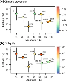
In Fig. 12, we plotted the values of the climatic preces-sion (defined as e × sin(ω − 180◦), with e the eccentricity and ω the precession), which modulates the Northern

Hemi-sphere insolation, and obliquity, which controls the temper-ature contrast between the high and low latitudes, relative to the SLPa-5 barycentre position, in order to analyse the relationship between the astronomical parameters and the SLPa-5 barycentre’s position. Climatic precession influences the SLPa-5 barycentre position in both longitude and lati-tude: when the climatic precession is high, the barycentre tends to move to the south-east (Fig. 12a). Obliquity mod-ulates the latitudinal changes in the SLPa-5 barycentre: high obliquities are associated with a SLPa-5 barycentre farther north (Fig. 12b). MIS3 has a climatic precession value sim-ilar to the CTRL one and a much higher obliquity than the CTRL one. Thus, the changes in MIS3 winds and productiv-ity related to insolation are mostly obliquproductiv-ity-driven (Fig. 12). Inversely, MIS4F has a similar obliquity to the CTRL one and a smaller climatic precession, which implies that the changes in monsoon intensity in MIS4F are related to preces-sion (Fig. 12). The Holocene simulations are influenced by both obliquity and precession, while the LGM, MIS4M and MIS4D simulations seem to reflect a stronger link with the obliquity signal than with the climatic precession (Fig. 12).

4 Discussion

4.1 The summer monsoon paradigm

In the simulations, the general paradigm stating that a stronger summer monsoon intensity induces a stronger up-welling and therefore increases marine productivity, is not always verified. Our results show that the characterisation of the summer monsoon intensity is probably insufficient to as-sess past productivity changes and vice versa (Fig. 9).

Our results for the summer productivity are consistent with the reconstructed productivity of Rostek et al. (1997). In their study, they analyse two marine sediment cores in the Ara-bian Sea: one in the south-east (5◦040N–73◦520E) and one in the upwelling region close to the Oman coast (13◦420N– 53◦150E). They show that palaeo-productivity in the south-eastern core was higher in glacial stages than in interglacial stages, which they interpret as the fingerprint of a stronger winter monsoon. In the other core, the productivity signal is more complex and they could find some glacial stages (e.g. stage 2) with high productivity, some interglacial stages with low productivity (e.g. stage 1) and stage 3 with high pro-ductivity. Similarly, in the simulations, in the central Arabian Sea, glacial productivity is higher than interglacial productiv-ity (except for MIS4F) (Fig. 8). In the western coastal Ara-bian Sea, the simulated MIS3 productivity is higher than the CTRL, while the other climates’ productivity is lower than CTRL. Hints on the sources of discrepancies between our results and the results of Rostek et al. (1997) and their inter-pretation of the productivity changes are given later in this section.

We explain the simulations’ summer productivity changes by analysing the variations in the wind forcing (Fig. 9).

70 75 80 85 90 95 100 24 25 26 27 28 Longitude Latitude

●

●

●

●

●

●

●

●

CTRL MH EH LGM MIS3 MIS4F MIS4M MIS4D_y 18 20 22 24 26 28 30 70 75 80 85 90 95 100 24 25 26 27 28 Latitude

●

●

●

●

●

●

●

●

CTRL MH EH LGM MIS3 MIS4F MIS4M MIS4D y 80 100 120 140 160 180 70 75 80 85 90 95 100 24 25 26 27 28

●

●

●

●

●

●

●

●

CTRL MH EH LGM MIS3 MIS4F MIS4M MIS4D −1.5 −1.0 −0.5 0.0 0.5 1.0 1.5 molC m−2 _yr-1 Coastal productivity (a) Position of the barycentres (b)

Coastal wind stress

(c) ₁₀-3 _{N m}−2 (d)Coastal wind stress curl 10-7 _{N m}−3

MH EH LGM MIS3 MIS4F MIS4M MIS4D CTRL Latitu de (°N) Longitude (° E) La tit ud e ( ° N ) Longitude (° E) Longitude (° E) La tit u de ( ° N )

Figure 11. (a) Position of the SLPa-5 barycentre for the eight simulations. Seasonal (JJAS) coastal (b) productivity (molC m−2yr−1), (c) wind stress intensity (10−3N m−2, y axis) and (d) wind stress curl intensity (10−7N m−3, x axis) as a function of the SLP barycentre longitude and latitude. Errors bars give standard deviation of the 100 summers. The dotted black box in panel (a) represents the region on which we zoomed for panels (b–d).

70 75 80 85 90 95 100 24 25 26 27 28

●

●

●

●

●

●

●

●

CTRL MH EH LGM MIS3 MIS4F MIS4M MIS4D y 70 75 80 85 90 95 100 24 25 26 27 28

●

●

●

●

●

●

●

●

CTRL MH EH LGM MIS3 MIS4F MIS4M MIS4D _y (a) (b)Obliquity −0.04 −0.02 0.00 0.02 0.04 21° 22° 23° 24° 25° Climatic precession Latitu de (°N) Longitude (° E) Latitu de (°N) Longitude (° E)

Figure 12.Mean (a) climatic precession (e · sin(ω − 180◦) where eis the eccentricity and ω − 180◦is the precession) and (b) obliq-uity values as a function of the longitude and latitude of the SLPa-5 barycentre for the eight climate simulations. Errors bars give the standard deviation of the SLPa-5 position over the 100 summers of each simulation.

Given the productivity changes in the different simulations, the summer monsoon intensity alone is not able to explain the changes in productivity and therefore we also investigate the changes in the monsoon pattern (Fig. 11).

The large-scale definition of the monsoon intensity, via 1TT, is mainly driven by astronomical changes. The sim-ulations with a strong summer monsoon either have a high obliquity, which enhances the temperature contrast be-tween low and high latitudes in summer (e.g. MIS3), or a small climatic precession that intensifies the summer inso-lation (MIS4F), or both (MH and EH) (Fig. 12) (Prell and Kutzbach, 1987). Simulations with a weak summer monsoon all have a small obliquity forcing (Fig. 12b). The local wind stress that affects productivity is tightly coupled to the mon-soon intensity (Fig. 9a, b) and is associated with a SLPa-5 barycentre movement to the north (Fig. 11c). This simulated latitudinal movement of the SLPa-5 barycentre, according to the monsoon intensity, is consistent with the study of An-derson and Prell (1992). In this study, the authors show that with a stronger monsoon the Somali Jet moves further north, which would indeed translate into a northward movement of the SLP barycentre (and inversely). In Fleitmann et al. (2007), the authors investigate the variations in the precipita-tion records of stalagmites located in Oman and Yemen. They link the changes in precipitation to the position and structure of the Inter-Tropical Convergence Zone (ITCZ), which af-fects the tropical climate. They explain that during the early Holocene, a northward movement of the mean latitudinal

po-sition of the summer ITCZ is responsible for the decrease in precipitation. Throughout the Holocene, they show that the ITCZ shifted southward concomitantly with a decrease in the monsoon precipitation, induced by the reduction in North-ern Hemisphere summer insolation (Fleitmann et al., 2007). The changes in the ITCZ position highlighted by Fleitmann et al. (2007) are consistent with our results, especially with the changes in latitude in the position of the SLPa-5 barycen-tre given a similar glacial or interglacial background state (Fig. 11).

Marine productivity is not only influenced by the wind stress but also by the wind stress curl (Anderson et al., 1992) and the latter is also strongly influenced in our sim-ulations by the glacial or interglacial state of the climate (Fig. 11). The glacial–interglacial distribution of the wind stress curl is associated with a longitudinal movement of the SLPa-5 barycentre: the SLPa-5 barycentre moves to the east in glacial climates and to the west in interglacial climates (Fig. 11d). Pausata et al. (2011), who analysed the effects of different LGM boundary conditions on the atmospheric cir-culation, indeed found that ice sheet topography is respon-sible for changes in many features of the SLP field, e.g. po-sition of lows and highs and their variability. Ivanova et al. (2003) also evoke an eastward shift in the low-level jet posi-tion in summer as a possible mechanism to explain some pro-ductivity changes in the eastern Arabian Sea. Furthermore, we showed that climatic precession can also act to move the SLPa-5 barycentre eastward (Fig. 12a) and therefore affect wind stress curl and productivity.

We find a valid physical explanation for our simula-tions’ productivity changes through the effects of the sim-ulations’ boundary conditions (astronomical parameters and ice sheets) on the monsoon intensity and pattern. However, even if the simulated summer productivity compares quite well with the data in Rostek et al. (1997) in the south-eastern Arabian Sea (except for MIS4F), there are more discrepan-cies with their second core in the western coastal Arabian Sea (core in the southern part of the our coastal area), and also when compared with the reconstructions in Bassinot et al. (2011) (core in the northern part of the coastal area) (Fig. 10). These differences can arise from several sources, the first one being linked to the area in which we computed our averages (Fig. 2a). Indeed, in Rostek et al. (1997) the core in the upwelling region is taken in the southern part of our coastal area (Fig. 2a) and the core close to the Oman coast in Bassinot et al. (2011) is located in the northern part of our coastal area (Fig. 2a). Productivity reconstructed by Bassinot et al. (2011) is high in the early Holocene and gradually de-creases throughout the Holocene, whereas, in our simula-tions, the Holocene productivity is low compared with the pre-industrial productivity. A closer look at the productivity changes in the MH simulation in Fig. 8a can reconcile our simulations and this reconstructed productivity. In the sim-ulated MH climate, the northern part of the coastal area ex-hibits a positive productivity change, whereas the southern

part of the coastal area is characterised by a negative produc-tivity change compared with the CTRL (Fig. 8a). Therefore, our results are coherent with the results of Bassinot et al. (2011) for the mid-Holocene since their core is located in the northern part of our coastal area where we simulate higher MH productivity than in CTRL. However, we do not observe this dipole-like pattern in the EH productivity (Fig. 6a), and consequently, the EH simulation does not agree with this reconstruction. In the EH simulation, we do not have the remnant Laurentide Ice Sheet that is supposed to be present at this time period (Licciardi et al., 1998). The simulation with this model version was not available at the time of our analyses. The addition of a remnant ice-sheet over Europe and North America in the EH has been shown in Marzin et al. (2013), to induce a southward shift of the ITCZ and a strengthening of the Indian monsoon. A southward shift of the jets would modify the large-scale pattern of the SLP and therefore the wind stress and wind stress curl effects on the Arabian Sea. Based on our findings, the addition of this resid-ual ice sheet would move the SLPa-5 barycentre to the south-east, which could increase the wind stress curl and therefore productivity (Fig. 11).

Another source of mismatch between our simulations and data resides in the fact that we looked at productivity and not at the export production that will eventually reach the bottom of the ocean. We also focused on the boreal summer season while it is often advanced that the winter monsoon is respon-sible for higher productivity in glacial climates compared with interglacial climates, e.g. for the south-eastern core pro-ductivity in Rostek et al. (1997). It is likely that the boreal winter productivity may also affect the overall recorded sig-nal in the sediments. In the next section, we especially dis-cuss the effect of seasonality on productivity.

4.2 Seasonality

Here, we investigate new palaeo-productivity reconstructions for the Arabian Sea and we compare them to our simulations. The simulations largely agree with the reconstructions, with glacial productivities that are higher than Holocene produc-tivities in the north-western Arabian Sea, even during boreal summer.

We use data from the sediment core MD04-2873 located at 23◦320N–63◦500E in the northern Arabian Sea on the Mur-ray Ridge (Böning and Bard, 2009) (Figs. 2a and 8, yellow

circle). This core is well dated by 14C dates from 50 kyr

to present and has a marked Toba Ash layer (74 kyr BP; Storey et al., 2012) giving a significant robust stratigraphic marker. The coccolithophores are well preserved and abun-dant at this location. Their assemblages are used to recon-struct palaeo-productivity by using a transfer function that has been designed for the Indian Ocean, including the Ara-bian Sea (Beaufort et al., 1997). Samples have been pre-pared by settling onto cover slips (Beaufort et al., 2014) ev-ery 10 cm for stratigraphic intervals covering 2000 years

MH EH LGM MIS3 MIS4F MIS4M MIS4D PP (molC m -2 yr -1) (a) MD04-2873 productivity (23°32 N–63°50 E ) 5 10 15 20 25 30 6 9.5 21 46 60 66 72

Time period corresponding simulations :

6 9.5 21 46 60 66 72 5 10 15 20 25 30 Time (kyr BP) TPP (molC m −2 yr −1) Annual roductivity

Northern Arabian Sea

(b) 6 9.5 21 46 60 66 72 5 10 15 20 25 30 TPP (molC m −2 yr −1) JJAS roductivity

Northern Arabian Sea

(c) 6 9.5 21 46 60 66 72 0 1 2 3 4 5 6 Time (kyr BP) EPC (molC m −2 yr −1)

Annual export production

Northern Arabian Sea

(d) 6 9.5 21 46 60 66 72 0 1 2 3 4 5 6 Time (kyr BP) EPC (molC m −2 yr −1) Time (kyr BP)

JJAS export production at 100 m

Northern Arabian Sea

(e)

Time (kyr BP)

at 100 m

Figure 13.Box plots of (a) yearly reconstructed productivity from core MD04-2873 in the north-western Arabian Sea and (b) annual total primary productivity (TPP), (c) summer total primary productivity, (d) annual export production (EPC) at 100 m and (e) summer export production at 100 m in the northern Arabian Sea (60–68◦E, 20–68◦N) for the Holocene and glacial time periods. The box plots highlight the median value (bold line), the first and the third quartiles (lower and higher limits of the box), and the 95 % confidence interval of the median (upper and lower horizontal dashes). The dots are extreme values that happened during the 100 years of simulation

above and below each time period simulated by the model. On average, six samples were studied by time intervals. Coccolithophore analysis was automatically generated by a software, SYRACO, that has been trained to recognise coccolithophores (Beaufort and Dollfus, 2004). Figure 13a shows the resulting palaeo-productivity for seven of the eight time periods we previously analysed. This recon-struction indicates that glacial productivity is higher than Holocene productivity in this core. At the core location, the effect of the boreal winter monsoon on productivity is known to be strong (Lévy et al., 2007). Consequently, the stronger winter monsoons during glacial time periods are often used to explain how glacial productivity can be higher than inter-glacial productivity (e.g. Rostek et al., 1997; Banakar et al., 2005).

In Fig. 13, we also plotted the box plots of simulated an-nual and summer (JJAS) productivity and export production at 100 m for the same time periods in the northern

Ara-bian Sea (60–68◦E, 20–28◦N). Our simulated annual and

boreal summer productivity shows smaller differences be-tween glacial and interglacial climates than the reconstruc-tions (Fig. 13a–c). The export production shows a clearer separation between the glacial and interglacial climates in both the summer and annual plots (Fig. 13d, e). The differ-ences between productivity and export production (Fig. 13b–

e) highlight that water column processes modify the recorded signal, which adds difficulties when comparing the model re-sults with data.

In all simulated climates, the mean boreal summer produc-tivity is lower than the mean annual producproduc-tivity (Figs. 8 and 13). This indicates that in this region in the simulations the mean boreal winter productivity is higher than the mean bo-real summer productivity. Indeed, in the simulations in the re-gion of the core boreal winter productivity accounts for more than 40 % of the annual productivity and boreal summer pro-ductivity accounts for more than 20 % (not shown). The hy-pothesis, stating that glacial productivity is higher than inter-glacial productivity because of a stronger winter monsoon, could explain the variations in this core (e.g. Banakar et al., 2005). However, the observed present-day seasonal cycle of productivity in the northern Arabian Sea shows equal con-tributions of the winter and summer seasons to the annual productivity (Fig. 2b), suggesting that the simulations may underestimate the boreal summer contribution to productiv-ity compared with the boreal winter contribution.

Interestingly, the annual and boreal summer productivity plots look alike, with higher glacial than interglacial produc-tivity in the model (Fig. 13). Since the summer monsoon is able to affect the north-western Arabian Sea, as seen in Fig. 2b, it contributes to the recorded signal in the sediment

(e.g. Caley et al., 2011). The boreal summer monsoon effect on the recorded signal is then non-negligible and we see that, even during the boreal summer season, the simulations show higher glacial than interglacial coastal productivity (Figs. 10 and 13), as well as in the central Arabian Sea (Fig. 8). Conse-quently, the boreal winter productivity is not the sole contrib-utor to the higher glacial productivity signal compared with the interglacial productivity in the model, even in the north-ern Arabian Sea.

5 Summary and perspectives

We use the coupled IPSL-CM5A-LR model to study the Ara-bian Sea palaeo-productivity in eight different climates of the past. We focus on the processes behind the boreal sum-mer productivity changes in the western coastal Arabian Sea. We show that a stronger Indian summer monsoon, which is mostly driven by higher NH insolation, does not necessarily enhance the Arabian Sea productivity.

We show that glacial climates can be more productive in boreal summer in the Arabian Sea compared with the pre-industrial climate (Figs. 8 and 10). Furthermore, the glacial climates are more productive than the early Holocene, which was supposed to be the most productive period in the region (Figs. 8 and 13). We found that the paradigm between mon-soon intensity and productivity is valid for MIS3 in the west-ern coastal sea: a stronger monsoon leads to more productiv-ity. The paradigm is also valid in the coastal Arabian Sea for the LGM, MIS4M and MIS4D simulations: a reduced mon-soon intensity leads to a reduction in productivity. However, this is not the case for the MH, EH and MIS4F simulations for which a stronger summer monsoon is associated with re-duced productivity.

Our analyses highlight the importance of considering the monsoon pattern, especially the position of the maximum wind intensity over the Arabian Sea. The mechanisms behind productivity changes are summarised in Fig. 14. We examine the monsoon pattern through the SLP barycentre position of the depression covering the summer monsoon regions (SLPa-5 barycentre). The SLPa-(SLPa-5 barycentre is moved to the east in glacial climates and far north in climates where the monsoon is enhanced (Fig. 11), which highlights the influence of the ice sheet cover (Pausata et al., 2011) and of the astronomical parameters (Anderson and Prell, 1992). The monsoon pattern affects the wind stress and wind stress curl efficiency to bring more or less nutrients to the surface layers. A change in the pattern can reduce or increase the area in which the winds are effective. This study also highlights the combined effects of wind stress and processes related to wind stress curl on pro-ductivity. Neither wind intensity nor wind stress curl alone can explain productivity changes.

We need to keep in mind that the model’s coarse resolu-tion does not allow for a very precise representaresolu-tion of the region dynamics. This may have altered the relative weight

Astronomical parameters Ice sheet cover

Monsoon

intensity Monsoon pattern

Wind stress Wind stress curl

Nutrients Primary production Export production SLPa-5 barycentre’s position

Figure 14.Identified seasonal (JJAS) processes behind productivity changes in glacial and interglacial climates. Bold lines highlight the major pathways.

of the processes related to wind stress and wind stress curl and can explain why the astronomical signal is weak in the productivity changes. Arabian Sea productivity in the CTRL simulation shows quite large differences with observations, especially for the high-coastal-productivity extension in the western Arabian Sea (Fig. 3a). This can result from the model’s coarse resolution, which prevents the representation of mesoscale processes such as eddies. These fine-scale pro-cesses are shown to be of importance for the coupling be-tween biology and physics (Resplandy et al., 2011). More-over, these mesoscale processes contribute strongly to the ex-port of nutrients offshore and thus can explain why our high-productivity area is more restricted to the coast than in the observations. From our set of simulations we cannot assess the effect of the underestimation of productivity on our re-sults. Our simulations may underestimate productivity levels and variations but since most of the main physical processes are represented, we can draw conclusions on the link between these processes and productivity and their changes through time. A way to overcome these limitations and to quantify their effects would be to work with several other models and to analyse the coupling between biology and physics in those different models.

We demonstrated that both changes in wind stress and wind stress curl can affect productivity on the timescales of thousands of years (Fig. 10). The same effects of changes in productivity from wind stress and wind stress curl can be found on the inter-annual timescale (Fig. 4). The relationship between changes in stress or curl and productivity is simi-lar to the one we found for the glacial–interglacial climate changes (Figs. 4 and 10). It could be interesting to further