HAL Id: hal-01944379
https://hal.archives-ouvertes.fr/hal-01944379
Submitted on 18 Nov 2020
HAL is a multi-disciplinary open access
archive for the deposit and dissemination of
sci-entific research documents, whether they are
pub-lished or not. The documents may come from
teaching and research institutions in France or
abroad, or from public or private research centers.
L’archive ouverte pluridisciplinaire HAL, est
destinée au dépôt et à la diffusion de documents
scientifiques de niveau recherche, publiés ou non,
émanant des établissements d’enseignement et de
recherche français ou étrangers, des laboratoires
publics ou privés.
natura
Pascal Milesi, Thomas Lenormand, Christophe Lagneau, Mylene Weill,
Pierrick Labbé
To cite this version:
Pascal Milesi, Thomas Lenormand, Christophe Lagneau, Mylene Weill, Pierrick Labbé. Relating
fitness to long-term environmental variations in natura. Molecular Ecology, Wiley, 2016, 25 (21),
pp.5483-5499. �10.1111/mec.13855�. �hal-01944379�
6
Molecular Ecology (2016) doi: 10.1111/mec.13855
1 2 3
4
Relating fitness to long-term environmental variations in
5
natura
7
8 PAS C A L MI L ESI,* T H O M A S L E N O RM A N D,† C H R I S T O PH E L A GN EA U, ‡ M Y L E` N E W E I LL* and 9 2 PIE R RI C K LAB B E´ *
10 *Institut des Sciences de l’Evolution de Montpellier (UMR 5554, CNRS-UM-IRD-EPHE), Universit´e de Montpellier, Place
11 Eug`ene Bataillon, 34095 Montpellier, Cedex 5, France, †CEFE UMR 5175, CNRS, Universit´e de Montpellier, Universit´e Paul- 12 Val´ery Montpellier, EPHE -1919 route de Mende, F-34293 Montpellier, Cedex 5, France, ‡Entente Interd´epartementale pour la 13 D´emoustication du littoral m´editerran´een, 34 rue du N`egue-Cat 34135, Mauguio, France
14 15
16 Abstract
17 Quantifying links between ecological processes and adaptation dynamics in natura
18 remains a crucial challenge. Many studies have documented the strength, form and
19 direction of selection, and its variations in space and time, but only a few managed to
20 link these variations to their proximal causes. This step is, however, crucial, if we are
21 to understand how the variation in selective pressure affects adaptive allele dynamics
22 in natural settings. We used data from a long-term survey (about 30 years) monitoring
23 the adaptation to insecticides of Culex pipiens mosquitoes in Montpellier area (France),
24 focusing on three resistance alleles of the Ester locus. We used a population genetics
25 model taking temporal and spatial variations in selective pressure into account, to
26 assess the quantitative relationships between variations in the proximal agent of
selec-27 tion (amounts of insecticide sprayed) and the fitness of resistance alleles. The response
28 to variations in selective pressure was fast, and the alleles displayed different
fitness-29 to-environment relationships: the analyses revealed that even slight changes in
30 insecticide doses could induce changes in the strength and direction of selection, thus
31 changing the fitness ranking of the adaptive alleles. They also revealed that selective
32 pressures other than the insecticides used for mosquito control affected the resistance
33 allele dynamics. These fitness-to-environment relationships, fast responses and
contin-34 uous evolution limit our ability to predict the outcome of adaptive allele dynamics in
35 a changing environment, but they clearly contribute to the maintenance of
polymor-36 phism in natural populations. Our study also emphasizes the necessity of long-term
37 surveys in evolutionary ecology.
38
39 4 Keywords: adaptation dynamics, insecticide resistance, population genetics model, selective
40 pressure variations, time-series
41 Received 27 June 2016; revision accepted 9 September 2016
42 43 44 45 46 47 48 49 50 51 52 53 54 3 Introduction
Determining how selective pressures shape the adaptive response of organisms in natura has been a crucial chal- lenge for 150 years and remains so today (Lewontin 1974; Endler 1986; Siepielski et al. 2009; Barrett & Hoek- stra 2011). One of the principal difficulties involved is the measurement of fitness in the field. Natural
Correspondence: Pierrick Labb´e, Fax: xx xxx; E-mail: pierrick. labbe@umontpellier.fr
selection has been thoroughly investigated at pheno- typic level, particularly since the development of multi- variate methods (Lande & Arnold 1983). Many studies have documented the strength, form and direction of selection (Conner 2001; Kingsolver et al. 2001; Hereford
et al. 2004) and its variation over space (reviewed in
Kawecki & Ebert 2004; Siepielski et al. 2013) and time (reviewed in Siepielski et al. 2009, 2011; Bell 2010; but
see also Morissey & Hadfield 2012). The interpretation 5
of these variations is hindered by a series of well- known issues (Mitchell-Olds & Shaw 1987; Rausher
C E : S eli n A ar th i R P E : S ak th iv el R . D is pa tc h: 1. 10 .1 6 N o. o f p ag es : 17 1385 5 M an us cri pt N o. M E C Jou rna l Code
1 1992; Bell 2008; Millstein 2008; Gallet et al. 2012;
2 Lenormand et al. 2015), including the impact of drift,
3 measurement error and trait plasticity. Another major
4 problem is that natural selection can vary at different
5 spatial and temporal scales. However, not all variations
6 are relevant: for example, variations in selection over
7 periods shorter than the generation time (e.g. between
8 life stages, Schluter et al. 1991; seasons, Benkman &
9 Miller 1996; or years for longer lived species, Schemske
10 & Horvitz 1989; Grant & Grant 1995) and distances of
11 less than the dispersal distance are not necessarily
rele-12 vant for adaptation, as they can miss important
trade-13 offs. Finally, natural selection may favour phenotypes
14 that can cope with rare (relative to the scale of
observa-15 tion) and extreme events that are difficult to sample
16 properly (Gutschick & BassiriRad 2003). Many of these
17 events are central to the functioning of the ecosystem
18 (fire, flood, storms, etc.) and must be understood if we
19 are also to understand adaptation (Karlin & Lieberman
20 1974; Grant & Grant 1993). Repeated sampling, over
21 sufficiently large geographical areas and time periods,
22 is therefore required to ensure that these events are
23 picked up.
24 Over and above these issues inherent to the
measure-25 ment of fitness in the field, there is another major
prob-26 lem: it is generally more difficult to link selection to its
27 causes than to quantify it (Wade & Kalisz 1990; Caruso
28 et al. 2003; Siepielski et al. 2009). Like finding a needle
29 in a haystack, it is indeed often extremely difficult to
30 identify the agent of selection precisely, let alone
deter-31 mine its quantitative relationship to fitness, as
pheno-32 typic and environmental variations are both complex
33 and multidimensional (Barrett & Hoekstra 2011). The
34 agent of selection affecting the variation in a particular
35 adaptive trait must be identified from a large number
36 of correlated and interdependent variables acting on a
37 similarly complex multivariate phenotype. Nevertheless,
38 in many cases, the agent of selection can be reasonably
39 inferred from field data (Bishop et al. 1975; Grant &
40 Grant 1995; Losos et al. 1997; Carlson & Quinn 2007 see
41 also references in Endler 1986) and further investigated
42 by experimentation (Bishop 1972; Reznick & Bryga
43 1987; Losos et al. 1997; Rundle et al. 2003; Bradshaw
44 et al. 2004).
45 However, the data required to assess the quantitative
46 link between environmental and fitness variations, that
47 is fine-scale measurements of well-identified agents of
48 selection over time and space, are not generally
avail-49 able (but see, e.g., Bishop et al. 1975; Grant & Grant
50 1995; Carlson & Quinn 2007). Adaptations to
environ-51 mental variation caused by humans (e.g. insecticide
52 resistance, Whalon et al. 2008; Norris et al. 2015;
antibi-53 otic resistance, Nsanzabana et al. 2010;
Gonzales-Can-54 dels et al. 2011; heavy metal tolerance, Janssens et al.
2009) constitute a useful system for investigating the fit- ness response to changes in the environment. In such cases, the agent of selection is easier to identify and could, in principle, be quantified. Furthermore, the adaptive responses described so far to these anthro- pogenic selective pressures have a simple genetic deter- minism and can thus be traced in natural populations. However, even in these cases, the link between environ- mental variation and fitness remains mostly qualitative, semiquantitative at best: even in the best known exam- ples, environmental variation is usually described in a binary fashion (e.g. mine vs pasture for Holcus lanatus, Macnair 1987; treated vs nontreated areas for insecticide resistance studies Lenormand et al. 1999), ignoring the continuous nature of the quantitative variation in selec- tion pressure (e.g. concentration of particles in coal smoke, heavy metals or pesticides). In this study, we aimed to go beyond this simplified description, provid- ing a quantitative explanation of the relationship between environmental variation (the agent of selection) and fitness in a natural setting.
We used insecticide resistance in Culex pipiens mos- quitoes as a case study. Organophosphate (OP) insecti- cides were used in the Montpellier area (South of France) to control mosquito populations until 2007, when they were replaced by Bacillus thuringiensis var. is-
raelensis (Bti) toxins in line with new EU regulations
(European Commission 2007/393/EC 2007). The resis- tance of Culex pipiens mosquitoes to OPs in this area has been monitored for more than 40 years, providing one of the best-documented examples of adaption to environmental modifications in natura.
Three different resistance alleles at the carboxyl ester-
ase encoding Ester locus (Ester1, Ester2 and Estrer4,
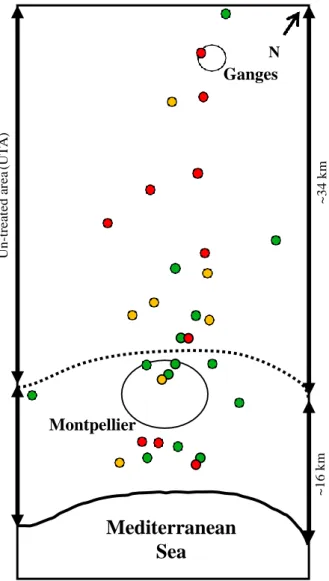
Guillemaud et al. 1998) have been reported to segregate in natural populations since the beginning of OP treat- ments. Like most new adaptations, these alleles are associated with pleiotropic deleterious effects, a selec- tive cost (Carri`ere et al. 1994; Chevillon et al. 1997; Berti- cat et al. 2002; Bourguet et al. 2004; Duron et al. 2006). Only the southern coastal strip of the Montpellier area was treated (Fig. 1). This resulted in antagonistic selec- tive pressures: resistance alleles were selected for in the southern treated area (hereafter referred to as the TA), as they allowed survival, and selected against in the northern untreated area (hereafter referred to as the UTA), due to their selective costs. Along a south–north transect, this results in the clinal distribution of their frequencies, making it possible to quantify the key parameters driving the long-term dynamics of Ester resistance alleles (e.g. migration, fitness coefficients, dominance Guillemaud et al. 1998; Lenormand et al. 1998, 1999; Labb´e et al. 2009), and their within-year vari- ations in relation to seasons and OP usage Lenormand
CO LO R T re a te d a re a ( T A )
1 RELATING FITNESS A ND ENVIRONMEN T IN N ATURA 3
1 2 3 4 5 6 7 8 9 10 11 12 13 14 15 16 17 18 19 20 21 22 23 24
Montpellier
25 26 27 28 29N
Ganges
described the strong correlations between variations in OP quantity and variations in allele frequencies. We then used a deterministic (i.e. no genetic drift) popula- tion genetics model to infer the specific fitness-to-envir- onment response of each Ester resistance allele by explicitly and quantitatively linking environmental vari- ation (i.e. the OP quantity, measuring the selective pres- sure variations) and fitness variation over the 1986–2012 period. It showed that even slight variations in insecti- cide doses induced changes in the strength and direc- tion of selection acting on the various resistance alleles, thus changing the outcome of their dynamics.
Materials and methods
Ester resistance alleles in the Montpellier area
Carboxyl esterases (COEs) catalyse cleavage of the ester bond of many molecules, including OPs (Oakeshott et al. 2005; Labb´e et al. 2011). In Culex pipiens, COE- mediated resistance is achieved by the overproduction of these enzymes due to upregulation or amplification of the genes encoding them (Rooker et al. 1996; Guille- maud et al. 1998). In the Montpellier area, three differ-
ent Ester resistance alleles have been described: Ester1
(upregulation), and Ester2 and Ester4 (gene amplifica-
tion).
As the various alleles are easy to identify by protein electrophoresis, their dynamics have been monitored
30 31 32 33 3416 35 36 37
Mediterranean
Sea
Fig. 1 Sampling transect map. Dots localize the various popu- lations sampled over the 1986–2012 period. Colours indicate the number of years of sampling for each site (1 – green; 2–4 – yellow; >4 –red). The studied transect crosses two areas: a coastal strip treated with OPs (TA) and an inland untreated
since 1986 in the Montpellier area, by sampling a simi- lar transect in late June or early July each year (Guille- maud et al. 1998; Lenormand et al. 1999; Labb´e et al. 2005; this study). This transect covers about 50 km and runs in a south–north direction from the Mediterranean to inland areas (Fig. 1). Insecticide use varies over this transect, with a treated area (TA) running along the coast and about 16 km wide (Labb´e et al. 2009) and an
38 area (UTA); the approximate transition between these two 39 areas is represented by the dotted line. The main towns in the 40 TA and UTA are indicated by black circles.
41
42 et al. 1999; Lenormand & Raymond 2000; Gazave et al.
43 2001).
44 The continuous sampling of mosquito populations
45 along the transect provided us with a data set of Ester
46 allele frequencies covering a period of about 30
consec-47 utive years. We also compiled and made use of data for
48 the amount of OPs used each year for mosquito control
49 in the TA. This data set provided us with a quantitative
50 spatial and temporal description of the environment,
51 which allowed measuring the causal link between
52 quantitative environmental variation and quantitative
53 variation in fitness for several alleles at a locus. We first
54
untreated area (UTA) further inland (Fig. 1). About ten larval Cx. pipiens populations have been collected almost each year along the sampling transect (some of the sites have changed, see Fig. 1) throughout the course of the survey. These larvae were reared to adult- hood in the laboratory, and adults were stored in liquid nitrogen for further analyses.
Insecticide treatments
In the coastal TA (Fig. 1), the local mosquito control agency (Entente Interd´epartementale pour la D´emoustica-
tion, EID) regularly treated larval breeding sites with
temephos (Abate®, Bayer), an OP insecticide, until 2007.
EID provided us with the total quantities used per year from 1990 to 2007 (Table 1). Un -t re a te d a re a (U T A ) ~1 6 k m ~3 4 k m
Ta b le 1 D at a co lle ct io n fr om 19 86 to 2 01 2 99 † 01 † 02 † 03 ‡ 04 ‡ 05 ‡ 06 ‡ 07 ‡ 08 ‡ 09 ‡ 10 ‡ 12 ‡ Y ea r 86* 87* .. . 90 91* 92 93* 95* 96* 98 00 To ta l — — .. . — — 8.82 — — 3.31 — — 1.95 — — 4.50 — — 2.31 — — 3.13 Np op Ni T 10 354 8.82 3 125 8.82 7 217 8.12 2 110 2.60 10 1203 1.49 7 512 2.58 8 411 3.40 12 736 4.30 9 521 3.62 8 464 1.64 8 464 2.46 9 526 2.65 8 466 0.18 8 464 0.11 7 406 0.00 4 236 0.00 13 722 0.00 9 582 0.00 14 2 85 19 The nu mb er o f p op ul ati ons c ol le ct ed (N pop ), the nu mb er o f i nd iv idu al s ana ly sed (Ni ) a nd the t ot al a m ou nt of O Ps a pp lie d (T ) e ac h ye ar in the tr ea te d ar ea a re pr es ented . F ro m 19 86 to 1 98 9, tr ea tme nt ap pl ic at io ns (i .e. the si ze o f the tr ea te d ar ea a nd the a m ou nts u sed) di d no t di ff er s ig ni fi ca nt ly fr om tho se in 1 99 0 (EI D 19 92 ; Gu ill ema ud et a l. 19 98 ). We ther ef or e a tt ri bu te d the s ame a mo unt of O Ps to the y ea rs fo r wh ic h thi s inf or m ati on w as mi ss ing (i ta lic s) . The d is tr ibu ti on of the ins ec ti ci de w ith in the t re ated a re a di d no t cha ng e si gn if ic an tl y betwe en 19 90 a nd 20 05 (Gu ill em au d et a l. 19 98 , t hi s stu dy, da ta n ot sh own). Af ter 2 00 7, temep ho s w as n o lo ng er u sed, th is p ro du ct be ing r ep la ced by Bt i, a mi xtu re o f t ox ins ex tr ac te d fr om B ac ill us th ur in gi en si s va r. i srael en si s. *Da ta fr om Gu ill em au d et a l. 19 98 . † Da ta f ro m L ab b´e et a l. 200 9. ‡Th is s tu dy, see Ta bl e S 1 (Su pp or ti ng inf or m at io n) . 1 Phenotyping 2
3 The 1986–2002 phenotype data set was already available
4 (Guillemaud et al. 1998; Labb´e et al. 2005, 2009). It was
5 extended by phenotyping 58 mosquitoes from each of
6 the 74 populations from 2003 to 2012. The Ester
pheno-7 type of each mosquito was obtained by starch gel
elec-8 trophoresis (Tris–malate–EDTA 7.4 buffer, Pasteur et al.
9 1988). Overproduced esterases are dominant over
non-10 overproduced esterases under our electrophoretic
con-11 ditions. The nomenclature and the correspondence
12 between genotypes and the observed phenotypes are
13 given in Table S1 (Supporting information).
14
15 Allele frequencies and clines
16
17 Allele frequencies and their support limits (equivalent
18 to 95% confidence intervals) were estimated from
phe-19 notypic data, independently for each population and
20 each year, using the maximum-likelihood approach
21 developed by Lenormand et al. (1999).
22 As the position and number of the sampled
popula-23 tions changed between years over the total period;
syn-24 thetic parameters summarizing the cline were thus
25 inferred to allow between-years cline comparisons. A
26 geometric cline of allele frequencies (pi) was fitted, by
27 maximum-likelihood methods (see below), to all the
28 samples for each sampling year. This cline, adapted
29 from Lenormand et al. (Lenormand et al. 1998), was
30 approximated by a negative exponential function: 6 7
31 p ¼ h · e—ðai ·x
2 Þ
ð1aÞ
i i
32
33 where hi is the maximum frequency of each allele i.
34 (MaxAF), ai describes the shape of the cline for allele i
35 and x is the distance to the sea. The parameters of this
36 descriptive cline thus represent and summarize the
37 observed data.
38 39
Population genetics model 40
41 To quantify the parameters influencing the allele
42 dynamics at the Ester locus, we modified the model
43 used in Labb´e et al. (2009). This model is deterministic;
44 that is, genetic drift was neglected: previous studies
45 suggested, in particular due to the large size of
mos-46 quito populations, that drift plays, at best, a minor role
47 in resistance alleles dynamics (Labb´e et al. 2005). It is a
48 stepping stone model (Lenormand & Raymond 1998,
49 2000; Lenormand et al. 1998, 1999) that considers 35
50 demes 2 km apart but connected by migration, and
51 implements three successive steps at each cycle (i.e.
52 each generation): reproduction, selection and migration.
53 As described by Lenormand et al. (1999), we considered
54 there to be 13 generations per year in Cx. pipiens from
94
97
1 RELATING FITNESS A ND ENVIRONMEN T IN N ATURA 5
1 southern France, corresponding to a total of 339 cycles
2 for the period 1986–2012.
3 4
5 Reproduction
6 The allele frequencies in each generation were
calcu-7 lated from those in the previous generation, assuming
8 panmixia independently in each deme, as inferred from
9 the observed phenotypic data (Labb´e et al. 2005). Each
10 deme was considered to be an infinite population (no
11 drift).
12 13
14 Selection
15 The fitness (wij) of a diploid genotype combining the
16 Ester alleles i and j depends on the selective advantages 17 (si and sj) and costs (ci and cj) of each allele. We
18 assumed codominance of advantages and of costs. wij
19 was thus calculated as follows:
20
21 wij ¼ 1 þ c½si þ 0:5ðsj — siÞ] — ½ci þ 0:5ðcj — ciÞ]; ð2Þ
22 where 1 is the fitness of a susceptible homozygote and
23 c a variable indicating whether the considered deme is
24 in the TA (c = 1) or the UTA (c = 0). Both the resistance
Parameter estimations
Three types of inferences were thus computed indepen- dently from the phenotypic data: (i) the observed resis- tance allele frequencies, inferred in each sample independently, to plot the data, (ii) synthetic cline parameters, describing the observed resistance allele frequency at any position on the transect, inferred for each year independently, and (iii) fitness parameters driving the resistance allele dynamics (and their relation to treatment data), inferred using the population genet- ics model: deterministic recursions generated the pre- dicted frequency of each allele at any point in time for the 1986–2012 period and at any position over the whole transect, for a given set of parameter values.
In each analysis, the inferred parameters allow com- puting the predicted phenotypic frequencies, which were then compared with the observed data of the rele- vant sample data set: (i) the phenotype frequencies in a given sample, (ii) the phenotype frequencies of all sam- ples of a given year and (iii) the phenotype frequencies of all samples.
To this end, we calculated the log-likelihood L of observing all the data:
25 advantage s and the selective cost c affect fitness in the
26 L ¼ X X X nijtlnðfijtÞ; ð3Þ
TA, whereas only c has an effect in the UTA. The
fre-27 quency of each genotype after selection was calculated
28 separately for each deme, as its frequency before
selec-29 tion multiplied by the ratio of its fitness to mean fitness
30 (Lenormand & Raymond 2000; Labb´e et al. 2009).
31 32
33 Migration 34
35 Migration between demes was calculated as an
approxi-36 mately Gaussian dispersal kernel with a
parent–off-37 spring distance standard deviation r = 6.6 km/generation1/2 (Lenormand et al. 1998). 39
40 Initial conditions 41
42 As described by Labb´e et al. (2009) and to allow more
43 flexibility, the eqn 1a was slightly modified to infer the
44 initial (i.e. in 1986) allele frequencies at the Ester locus
45 as:
46 p ¼ h · e—ðai·x2 þbixÞ
ð1bÞ
t i j
with nijt and fijt the observed number (from phenotyp-
ing data) and the predicted frequency (from allelic fre- quencies/cline/model parameters), respectively, of individuals with phenotype i in population j at time t.
It was simultaneously maximized (Lmax) for all inferred
parameters of a given equation/model over the whole relevant data set, with a simulated annealing algorithm (Lenormand & Raymond 1998, 2000; Lenormand et al. 1998, 1999; Labb´e et al. 2009).
For each parameter, the support limits (SL) were cal- culated as the minimum and maximum values that the parameter could take without significantly decreasing the likelihood (Labb´e et al. 2009); SL are roughly equiv- alent to 95% confidence intervals. Concretely, the upper
(pmax) and lower (pmin) SL for each parameter p were
inferred while all other parameters were allowed to change, ensuring that we find the actual pmax and pmin
in the range of the multidimensional parameter land- scape. We used the same equation/model and the same
i i
47 simulated annealing method, but instead of maximizing
48 where bi is an additional parameter defining the slope
49 of the cline. As the Ester2 allele was not yet present in
50 1986, we introduced it tapp2 generations after 1986, at a
51 frequency of 0.01 in all demes in the TA (tapp2 is
esti-52 mated in the model).
53 The various parameters were estimated by a
maxi-54 mum-likelihood approach.
L, we maximized (pmax) or minimized (pmin) the values
of p for which the likelihood was not significantly dif-
ferent from the maximum likelihood (i.e. Lmax minus
1.96).
Overdispersion was calculated for each model as the residual deviance D = —2L divided by the residual degrees of freedom (Dd.f.). The percentage of the total
38
1 deviance explained by a model was calculated as %
2 TD = (Dmax — Dmodel)/(Dmax — Dmin), with Dmax and
3 Dmin the maximal and the minimal deviance,
respec-4 tively. Recursions and likelihood maximization
algo-5 rithms were written and compiled with LAZARUS v1.0.10
6 (http://www.lazarus.freepascal.org/).
7 8
9 Hypothesis testing using the population genetics
10 model
11 The model developed by Labb´e et al. (Labb´e et al. 2009)
12 considered 13 parameters (Table 2): two selection
coeffi-13 cients (si and ci) for each resistance allele i, in addition to
14 three initial allele frequency parameters (hi, bi, ai) for
We added to this original model several parameters, which allowed testing for various hypotheses about how environmental variations could affect the Ester dynamics:
1 to test for reductions in the fitness costs of Ester alle- les (cri), the model was allowed to fit different selec- tive costs after generation tcost, a parameter estimated
simultaneously with the others; from generation tcost
onwards, ci was replaced by ci — cri in eqn 2 (see Methods section ‘Migration–selection model’).
2 to estimate the impact of selective pressures other than the insecticide used for mosquito control, the selective advantage (si) was broken down into two terms, siT and s0: siT is the advantage due specifically
15 1 4 2 i 0
Ester
16 and Ester ; Ester was not yet present in 1986, so to resistance to the OPs used for mosquito control; si
that the last parameter was its date of appearance (tapp2).
17 18 19
20 Table 2 Best population genetics model
is the selective advantage of the resistance alleles due
21 Parameters Estimate (SL) F (Dd.f.) 22 23 24 25 26 27 28 29 30 31 32 33 34 35 36 37 38 39 40 41 42 43 44 45 46 47 48 49 50 51 52 53 54 8 1 2
The estimated value of the different parameters is given with their associated support limits (SL). The significance of each parameter (for their description, see Methods section ‘Population genetics model’ and ‘Hypothesis testing using the population genetics model’) was then tested by removing it and comparing the likelihood of the resulting model with that of the best model, using LRTod (n.snon-
significant, *P < 0.05, **P < 0.01, ***P < 0.001). The LRTod (F) statistic and the difference in the number of degrees of freedom (Dd.f.)
are also indicated for each parameter. The fitness of each resistance allele (wi) before OP removal and relative to the susceptible allele
(w0 = 1) is also given, for both the TA and UTA. Finally, the log-likelihood (L), the total deviance explained (%TD) and the overdis-
persion (Od) of the best model are indicated. Parameters labelled with # were not included in the model described by Labb´e et al. (48) (see Methods section ‘Hypothesis testing using the population genetics model’).
Initial conditions (1986) MaxAF h1 0.55 (0.41–0.70) 19 314 (1)***
Slope Shape b 1 a1 0.11 (0.07–0.15) 0.00 (0.00–0.00) 96 (1)*** 0 (1)n.s
Ester2 appearance generation
MaxAF Slope Shape h4 b4 a4 tapp2 0.04 (0.02–0.07) 0.02 (0.00–0.08) 0.00 (0.00–0.00) 55 (35–65) 90 467 (1)*** 3 (1)n.s 0 (1)n.s 8592 (1)***
Costs change generation# tcost 261 (260–267) 15 (4)**
Selective costs before tcost c1 0.08 (0.07–0.10) 196 (1)***
c2 0.11 (0.08–0.17) 67 (1)***
c4 0.04 (0.03–0.05) 183 (1)***
#
Selective cost reduction after tcost cr1 0.02 (0.003–0.05) 6 (1)*
cr2 cr4
0.05 (0.01–0.10)
0.00 (0.00–0.01) 5 (1)* 0 (1)n.s
Selective advantages Treatment s1T 0.22 (0.19–0.26) 8 (3)*
s2T 0.32 (0.22–0.43) 72 (3)*** Background# s4T s0 s0 0.21 (0.14–0.28) 0.13 (0.08–0.18) 0.08 (0.00–0.16) 77 (3)*** 325 (1)*** 2 (1)n.s s0 4 0.12 (0.09–0.14) 217 (1)*** Dose–response parameters# d1/m1 2.13 (1.96–2.39)/80.0 (2.25–80) 8 (2)* d2/m2 1.95 (1.79–2.27)/40.0 (2.30–40) 65 (2)*** d4/m4 3.66 (3.17–4.20)/1.26 (1.12–2.1) 77 (2)*** Relative fitnesses (w1:w2:w4) TA 1.14:1.19:1.16 UTA 0.92:0.89:0.96 %TD 92.5 Od 1.47 '
1 RELATING FITNESS A ND ENVIRONMEN T IN N ATURA 7
0
1 to the presence of other agents of selection. si could
2 thus remain >0 even in the absence of insecticide
3 treatment.
4 3 to take into account the quantitative variations in OP
5 insecticide use over the 1986–2012 period, the
selec-6 tive advantage of Ester resistance alleles due to
mos-7 quito control (siT) was calculated as a function of the
8 amount of OPs used each year t (Tt).
9
10 We took above points 2) and 3) into account by
calcu-11 lating the selective advantage si (eqn 2) as:
12
13 si ¼ siT · fðTtÞþ si; ð4Þ
14 We considered a flexible functional form for f(Tt)
15 (allowing for possible nonlinearity), assuming that it
16 was monotonically increasing (selection intensity
17 should increase with insecticide dose). We thus used a
18 logistic function: fðTtÞ ¼ 1 — ð1=1 þ em
i ·ðbi þTt ÞÞ. This
sig-19 moid curve is centred on dose bi and has a maximum
20 slope proportional to mi; these parameters are hereafter
21 referred to as the dose–response parameters. We fitted
22 mi and bi independently for each allele i but the model
23 was constrained to accept only mi/bi combinations for
24 which f(Tt) < 0.0001 when Tt = 0; so that f(Tt) = 0 in
25 the absence of treatment. Thus, the advantage of the
26 resistance alleles in the presence of mosquito control
27 treatment varied from ~0 at low doses to siT at high
28 doses.
29 30
Tests and control for overparameterization 31
32 The significance of each parameter was tested by
com-33 paring the likelihoods of the best model and of a
34 model in which the tested parameter was withdrawn,
35 using likelihood-ratio tests corrected for overdispersion
36 [LRTod; (Anderson et al. 1994)]. The best model
37 includes 26 parameters. This number is fairly small
38 given the size of the data set (994 phenotypic
frequen-39 cies along a 50-km transect over 27 years,
correspond-40 ing to over 8500 individuals sampled), but there is
41 always a risk of overparameterization. One way to
42 check for overparameterization is to check for structure
43 in the model residuals: if they are randomly
dis-44 tributed, the inclusion of additional parameters would
45 be superfluous.
46 We tested in particular whether the inclusion of the
47 dose–response parameters resulted in
overparameteriza-48 tion. A simplified model was implemented; this model
49 included only a qualitative description of the
environ-50 ment, due to modification of the selective advantage
51 (si), as si = siT + s0i. The risk of overparametrization was
52 then assessed by comparing the correlations of the
53 residuals of the simplified and best models with the
54 amounts of OPs applied.
For the period during which OPs were used, we cal-
culated the simplified model residuals ej for all data
points j as: ej = pjobs — pjmod, where piobs is the allelic frequency estimated from phenotypic data and pimod the allelic frequency estimated with the model. Correla-
tions between ej and Tt were tested by calculating Pear-
son’s product–moments (R software v.3.1.1 http://
www.R-project.org/).
Results
The 1986–2012 data set
Insecticide resistance. We estimated allele frequencies
along the surveyed transect (Fig. 1), by phenotyping 58 individuals per sampled population per year by starch gel electrophoresis (Table S1, Supporting information). Over the entire 1986–2012 period, we analysed data from 8519 individuals from 142 sampled populations, with a mean of eight populations sampled per year (Table 1). The numbers of individuals displaying each phenotype have already been published for the 1986 to 2002 samples (Guillemaud et al. 1998; Labb´e et al. 2005). For samples collected from 2003 to 2012, these data are presented in the Table S2 (Supporting information).
Insecticide treatments. The local mosquito control agency
(EID) had used OPs for pest control since 1969. They are used essentially from March to October (seaside tourism), which has been shown to affect the allele dynamics within a year (Lenormand et al. 1999). The spatial distribution of treatments did not change signifi- cantly over time (Labb´e et al. 2009; supplementary material; EID, personal communication). However, the amounts of OPs used annually in the treated area (TA) varied over the 1986–2012 period (Table 1). They varied according to changing general treatment policies: (i) first, from 1986 to 1991, temephos (an OP insecticide) was the only insecticide used, with relatively large
quantities sprayed, around 8 L/km2 (EID 1992; Guille- 9
maud et al. 1998); unfortunately, precise information is unavailable for the years before 1990: the amounts used probably varied slightly around the mean, due to treat- ment adjustment to weather-linked variations in mos- quito densities, but these variations were limited (EID 1992); (ii) in 1992, EID began to use new bacterial toxins [first, Bacillus sphaericus (Bs) then Bacillus thuringiensis var. israelensis (Bti)], and the amount of temephos used was decreased by a factor of more than two, to 1.5–
4.5 L/km2, with a mean value of about 3 L/km2; these
variations again probably result from treatment adjust- ment (Table 1); (iii) finally, the amount of temephos applied was substantially decreased again in 2006 and
2007 (<0.2 L/km2), and this product was completely
1 2 3 4 5 6 7 8 9 10 11 12 13 14 15 10 16 17 18 19 20 21 22 23 24 25 26 27 28 29 30 31 32 33 34 35 36 37 38 39 40 41 42 43 44 45 46 47 48 49 50 51 52 53 54
withdrawn after 2007, in line with new European legis- lation (Table 1); OP insecticides have now been entirely replaced by Bti.
Environmental variations affect the dynamics of Ester alleles
Using this unique data set, we were able to carry out a precise survey of the dynamics of Ester resistance alle- les.
First, the typing method gives only access to the phe- notypes in each sample: we cannot differentiate Ester resistance allele homozygotes from heterozygotes carry- ing one resistant and one susceptible alleles (see Meth- ods and Fig. S1, Supporting information). We thus used a maximum-likelihood approach to infer the allelic fre- quencies from these observed phenotypic frequencies, independently for each sample (Fig. S3, Supporting information).
Secondly, the position and number of the sampled populations changed between years over the total per- iod; synthetic parameters were thus required for between-years cline comparison. A geometric cline was thus fitted for each resistance allele to the observed phenotypic data of all samples of each year (eqn 1a, Methods section ‘Allele frequencies and clines’, Table S4, Supporting information). These clines provide us for each resistance allele i with its maximum fre-
quencies, or MaxAFi (i.e. its frequency at the coast), and
a parameter ai describing the shape of the cline, with
their associated support limits (see Methods section ‘Parameter estimations’). Both approaches provide purely descriptive representations of the spatial distri- bution and dynamics of the resistance alleles.
Resistance allele frequencies are correlated with the amount of OPs applied. As previously reported (Guillemaud et al.
1998; Labb´e et al. 2009), during the period of OPs use,
Ester1 was initially replaced by Ester4, until the invasion
of Ester2 in the 1990s. As Ester2 fitness appeared
superior to that of the other resistance alleles in the presence of insecticide, Labb´e et al. (2009) fore- told its increase in frequency (providing continuation of the OP treatments), eventually reaching fixation. Unex- pectedly, the frequency of Ester2 actually peaked in 2002, even
since OPs were still used until 2006; there- after, the Ester allele frequencies remained globally stable until 2005, with some marked differences between years (Fig. 2).
We investigated whether variations in the amounts of OPs applied could account for these allele frequency variations and for Ester2 not increasing further in fre-
quency. We first focused on the 1995–2008 period, when
all three resistant alleles were present in the area stud- ied and the amount of OPs applied ranged from 0.11 to
4.5 L/km2 (Table 1). There is on average 13 mosquito
generations per year, and several studies have shown that the selection–migration equilibrium is rapidly restored each year, after insecticide treatments resume in spring (Lenormand et al. 1999; Labb´e et al. 2009); we thus chose to directly analyse the relations between the summer Ester allele frequencies and the annual amount of OPs. Globally, Ester allele frequencies (resistance and susceptible alleles) in a given year were significantly correlated with the amounts of OPs used in the previ- ous year (Fig. 3), but not with those used in the same year (Table S5, Supporting information). A highly sig- nificant negative correlation was found between suscep-
tible allele (Ester0) frequencies at the sea and the
amounts of OPs applied the previous year (Pearson’s coefficient correlation r = —0.81, t = —4.16, d.f. = 9,
P < 0.01, Fig. 3A). However, different correlations were
observed when each resistance allele was considered separately. The MaxAFs of the Ester2 and Ester4 alleles
were correlated with the amounts of OPs used (r = 0.74,
t = 3.33, d.f. = 9, P < 0.01 and r = 0.70, and t = 2.95,
d.f. = 9, P < 0.05, respectively, Fig. 3B), but the correla-tion was not significant for Ester1, despite a similar
trend being identified (r = 0.37, t = 1.2, d.f. = 9,
P = 0.26, Fig. 3B). If we considered the 1986–2008
period (i.e. when OPs were used), the frequency of the Ester1 allele was greatly affected by the decrease in
the amounts of OPs used after 1991 (from 8.12 to
3.31 L/km2, Table 1 and Fig. 2). These relations were
further investigated, by considering the allele frequen- cies directly inferred from the phenotypic data, over the whole transect, for the 1986–2008 period. Similar corre- lations were identified, demonstrating the relation between the resistance allele frequencies and the year- to-year variation in selective pressure on the whole transect (not only in the TA close to the coast; Fig. S6, Supporting information).
Resistance allele frequencies decreased after the withdrawal of OPs, but are now moving towards a new equilibrium. A
major shift occurred around 2005. Anticipating the Eur- ope-wide ban on OPs due to come into force in 2007, EID substantially decreased the amounts of OPs used between 2005 and 2007, when these products were withdrawn completely. As expected, the withdrawal of OP insecticides had a considerable effect on the dynam- ics of the Ester resistance alleles. After 2005, MaxAFs decreased very rapidly, with the frequencies of all the resistance alleles together falling from 0.85 to 0.37 between 2005 and 2010, before stabilizing again. The withdrawal of OPs thus led to a 56% decrease in
1 RELATI NG FITNESS AND ENVIRONMEN T IN N ATURA 9 Al le le f re q u e n c y a t th e s e a ( x = 0 k m) Al le le f re q u e n c y
1 (A) Fig. 2 Ester resistance allele dynamics
2 0.7 3 4 5 6 7 8 0.4 9 10 11 12 13 14 0.0 1986 1990 1994 1998 2002 2006 2010 15 Years 16
over the period 1986–2012 in (A) time and (B) space. (A) Evolution of the resis- tance allele frequencies from 1986 to 2012. For each sampled year, the dots represent the maximum allele frequen- cies (MaxAFs, i.e. at the sea) for Ester1
(blue diamonds), Ester2 (red squares) and
Ester4 (green triangles), synthetizing the
observed phenotypic data. The evolution of the allele frequencies predicted by the best population genetics model (complete set of parameters with the maximum likelihood) is represented by the solid lines for the resistance alleles and by the grey dashed line for the susceptible. The grey vertical dashed line indicates the date at which the model re-estimated
17 (B) 0.8 18 0.6 19 20 0.4 21 0.2 22 1986 0.8 0.6 0.4 0.2 1995
the cost of each resistance allele (tcost).
(B) Distribution of Ester resistance allele frequencies along the sampling transect. Dots represent the allele frequencies (with their support limits) inferred from the observed phenotypic frequencies for each sampled population. Lines represent
0 0 10 20 30 40 50 24 25 0.8 2005 26 0.6 27 28 0.4 29 0.2 30 0.0 31 0 10 20 30 40 50 0 0 10 20 30 40 50 0.8 2012 0.6 0.4 0.2 0.0 0 10 20 30 40 50
the frequency cline predicted by the best population genetics model. The colour code is conserved. Only four representa- tive years are figured (1986, 1995, 2005 and 2012, see Fig. S3, Supporting infor- mation for the others).
32 Distance from the sea (km)
33 34
35 resistance allele frequency, highlighting the high
selec-36 tive costs of these alleles.
37 Over the entire sampling transect, all Ester allele
fre-38 quencies followed a similar clinal distribution until
39 2005 (Labb´e et al. 2009; and Fig. S3 and Table S4,
Sup-40 porting information). After 2005, the overall decrease in
41 the frequency of all resistance alleles softened these
cli-42 nes (i.e. the frequencies became more homogeneous
43 between TA and NTA), as expected, due to spatial
44 homogenization of the environment, before a new
stabi-45 lization between 2010 and 2012 (Figs 2 and S3 and
46 Table S4, Supporting information). Consequently, in
47 2012, Ester1 and Ester2 frequencies appeared to be
uni-48 form and low (around 0.01) over the entire transect: ai
49 parameters (see Methods section ‘Allele frequencies and
50 clines’ eqn 1a), which describe the shape of the clines,
51 were not significantly different from zero (LRTod,
52 F = 0.64, Dd.f. = 1, P = 0.43 and F = 0.88, Dd.f. = 1,
53 P = 0.48, respectively, for Ester1 and Ester2). By contrast,
54 the clinal shape remained significant for Ester4 (a4 > 0,
LRTod, F = 10.11, Dd.f. = 1, P < 0.001) (Fig. S3,
Support-ing information). The frequency of this allele was rela- tively high over the entire transect, stabilizing at about 0.35 close to the sea and 0.16 inland (Fig. S3, Supporting information).
Quantifying the effects of environmental variations on fitness
Changes in fitness costs following OP withdrawal. One pos-
sible explanation for the persistence of resistance alleles after the withdrawal of OPs is changes in their fitness costs. We tested this hypothesis by fitting a selective cost reduction (cri) after tcost generations, a number of
generations also estimated by the model: the selective cost of the allele i after tcost is thus ci — cri (see Methods section ‘Hypothesis testing using the population genet- ics model’, Table 2). Despite the low frequencies of the
Ester1 and Ester2 alleles, which reduces the statistical
power, the best fit suggested a significant decrease in
CO
LO
R
1 2 3 4 5 6 7 8 9 10 11 12 13 14 15 16 17 18
19 their associated costs: respectively, cr1 = 0.02, that is a
20 25% reduction (LRTod, F-test = 6, Dd.f. = 1, P = 0.02)
21 and cr2 = 0.06, that is over 50% reduction (LRTod,
F-22 test = 5, Dd.f. = 1, P = 0.02) after tcost = 261 generations
23 (Table 2). This number of generation corresponds to
24 year 2006, when the amounts of OPs used were
25 strongly decreased, anticipating the ban on these
prod-26 ucts (Table 1 and Fig. 2). However, no significant
27 change in the cost of Ester4 was detected (cr4 = 0.00;
28 Table 2).
29 Previous studies have suggested that the level of
30 amplification of some Ester resistance alleles may vary
31 (i.e. copy number variation) in response to selection
32 pressures, with larger numbers of copies resulting in
33 higher resistance, but also in higher costs (Weill et al.
34 2000; Berticat et al. 2002). Both Ester2 and Ester4 result
35 from amplifications (whereas Ester1 results from the
36 constitutive overexpression of a single copy). We
there-37 fore also quantified the level of amplification of these
38 alleles, before and after the withdrawal of OPs, by
39 quantitative real-time PCR on genomic DNA (for
40 details, see Appendix S7, Supporting information).
41 However, no change in amplification level was detected
42 for either Ester2 or Ester4 (Appendix S7, Supporting
43 information).
44
45 Mosquito control treatments are not the only selective agent.
46 Another explanation for the persistence of the Ester
47 resistance alleles after OP withdrawal could be the
pres-48 ence in the environment of others compounds that
49 could select these alleles. To test this hypothesis, the
50 selective advantages of the resistance allele in the
51 model, si, were partitioned into a selective advantage siT
52 due to the OPs used for mosquito control (for which we
53 know the doses used in the years studied) and another
54 component, denoted s0
i, corresponding to the potential
effects of other selective pressures (see Methods section
‘Genetic model’, eqn 4). The s0
i values estimated were
significantly different from zero for Ester1 and Ester4 (re-
spectively, s0
1 = 0.13, LRTod, F-Test = 325, Dd.f. = 1,
P < 0.001 and s0
4 = 0.12, LRTod, F-Test = 219, Dd.f. = 1,
P < 0.001), but not for Ester2 (Table 2). It thus appeared
that Ester1 and Ester4 still conferred a selective advan-
tage, even after the withdrawal of OPs. The mosquito control treatments were therefore not the only selective agents acting on these alleles.
Fitness-to-environment relationships shape resistance allele dynamics. For quantification of the fitness-to-environ-
ment responses of the various alleles, the selective advantage due to mosquito control (siT) was calculated as a logistic function of the amounts of OPs used in each year t (Tt) over the period 1986–2012, with the addition of two dose–response parameters for each allele (see Methods section ‘Genetic Model’, 3). This best model fitted the data significantly better than the
simplified model with constant siT (see Methods section
‘Tests and control for overparametrization’; LRTod, F-
test = 33, Dd.f. = 6, P < 0.001).
Despite the highly significant result obtained, we checked whether the estimation of the dose–response parameters could have been driven by a few outlier samples. We ruled out such overparameterization by analysing the residuals of both the simplified and best models, with respect to the amounts of OPs applied (see Methods section ‘Tests and control for over- parametrization’). The residuals of the simplified model appeared to be structured and correlated with OP levels (r = 0.15, t = 2.7, d.f. = 324, P = 0.007), whereas those of the best model were not (r = 0.09, t = 1.7, d.f. = 324,
P = 0.095; Fig. S8, Supporting information). Together
with the correlations illustrated in Fig. 3, this confirms
CO LO R A ll el e fr eq u en cy (A) 0.8 r = –0.81** (B) 0.8 0 r = 0.371 n.s. ; r = 0.742 **; r = 0.704 * 0.4 0.4 0.0 0 1 2 3 4 0.0 5 0 OP quantities (L/km2) 1 2 3 4 5
Fig. 3 Ester allele frequencies vs amounts of insecticide used for (A) the susceptible allele and (B) the resistance alleles. The data
points indicate the allele frequencies close to the sea, inferred from phenotypic data. They are presented as a function of the amounts of OPs used in the previous year. (A): for Ester0 (black crosses) and (B): for Ester1 (blue diamonds), Ester2 (red squares) and Ester4
(green triangles). Straight lines represent the linear regressions between the two factors. The correlation coefficient ri (Pearson’s pro-
duct–moment correlation) between fi and the amount of OPs is provided, together with a P value indicating the significance of this
1 RELATI NG FITNESS AND ENVIRONMEN T IN N ATURA 11 R el at iv e fi tn es se s
1 that adding the dose–response parameters captured
2 actual fitness responses to dose variations and that this
3 improvement in fit was driven by the bulk of the data.
4 The parameter estimates indicated that the
fitness-to-5 environment responses differed between the Ester
resis-6 tance alleles (Fig. 4A): the selective advantages of these
7 alleles were differently affected by the variations in OP
8 quantities, confirming the correlations observed (Figs 3
9 and S6, Supporting information). The advantage of all
10 alleles was significantly and positively dependent on
11 OP levels (Ester1: LRTod, F-test = 8, Dd.f. = 2, P = 0.021;
12 Ester2: F-test = 66, Dd.f. = 2, P < 0.001 and Ester4:
13 F-test = 78, Dd.f. = 2, P < 0.001). However, the
fitness-14 to-environment response was steep for Ester1 and Ester2
15 (Fig. 4A): they appeared to be disproportionately
16 affected by slight variations in treatment in the 0 to
17 ~2 L/km2 range, but expressed their full advantage for
18 higher OP levels (Fig. 4A). By contrast, Ester4 was
19 affected over the whole 0 to 9 L/km2 range, but the
20 curve was smoother than for the other two alleles
21 (Fig. 4A).
22 Overall, this quantitative analysis suggests that the
23 fitness of the various resistance alleles is finely tuned to
24 quantitative changes in the amounts of OPs applied,
25 but also depends on changes in costs and on other
26 selective forces. The overall net effect was that the allele
27 with the highest fitness in the TA differed between
28 treatment intensities (Fig. 4B): Ester2 was more
29 30 31 (A) 32 33 34 35 36 37 38 39 40
advantageous at moderate to high doses of OPs,
whereas Ester4 and Ester1 were more advantageous at
low doses. However, Ester4 was the fittest resistance
allele in the UTA, due to its lower fitness cost (Table 2). Following the withdrawal of OPs, and thanks to contin-
uing secondary sources of selection, Ester1 and Ester4
appeared to confer similar and higher levels of fitness in the former TA (Fig. 4B). In the UTA, Ester4 remained
the fittest resistance allele, despite the decrease in the fitness cost of Ester1 and Ester2 (Table 2).
Discussion
To investigate how the variations in the amounts of OPs applied (i.e. selection intensity) affected the dynamics of the Ester resistance alleles (i.e. the adap- tive alleles), we first needed a quantitative description of the environment at a scale compatible with the scale at which the allele frequency variations were mea- sured. Fortunately, the treated area was only slightly greater than the area over which mosquitoes can dis- perse, so the heterogeneous distribution of selection intensities within the treated area (due to spatial varia- tions in insecticide use) could be ignored. We were also able to ignore the within-year variations, because such variations were not directly relevant to the long- term trend: no insecticide treatment occurred from October to March–April (leading to a decrease in
Fig. 4 Fitness-to-environment relation- ships and relative fitness of Ester alleles in the treated area over the 1986–2012 period. (A) The relative fitnesses of the different Ester alleles are represented as a function of the OP quantities (L/km2),
Ester0 (susceptible allele) – dashed black
line, Ester1 – blue line, Ester2 – red line
and Ester4 – green line. (B) The solid
lines represent the relative fitness (left axis) in the insecticide-treated area (TA)
(B) 1.3 10 41 42 43 8 44 45 6 46 47 1.1 48 4 49 50 2 51 52 53 0.9 0 54 1986 1992 1998 2004 2010
for each resistance allele (Ester1 in blue,
Ester2 in red and Ester4 in green), esti-
mated from the best model (with treat- ment-dependent fitnesses). The dotted line represents the fitness of the suscepti- ble allele (Ester0 in black, w0 = 1). For
each year, fitness is calculated as: 1 + siT + s0i - ci with siT, s0i and ci the
advantages (depending on the amount of OPs applied or other selective pressures) and the cost of the allele i (equal to
ci — cri after tcost, see text), respectively.
The barplot shows the total amount of OPs (L/km2, right axis) used each year
in the treated area over the 1986–2012 period. O P s q u a n ti ty ( L /k m 2) CO LO R
1 resistance allele frequency during this period due to
2 the fitness costs of these alleles, Lenormand et al. 1999;
3 Raymond et al. 2001), but it was previously shown that
4 a selection–migration equilibrium was rapidly reached
5 each year between susceptible and resistance alleles,
6 after a few rounds of treatment (Lenormand et al.
7 1999; Labb´e et al. 2009). We also took into account the
8 total amounts of OPs used in the TA in each sampling
9 year (therefore not taking into account the precise
tim-10 ing of treatment during the year). Thus, spatial and
11 temporal variations in selective pressure were
12 described quantitatively, at scales relevant to the
long-13 term trends. Consistent with this description of the
14 environment, we used Ester frequency data from only
15 one season (early summer). Fitness estimates based on
16 these data must therefore be considered as averages
17 over the treatment period.
18
19 Adaptive responses are tuned to selective pressure 20
variations
21
22 Annual OP use was found to be strongly correlated
23 with summer resistance allele frequencies: the resistance
24 allele frequencies in any given year were more strongly
25 related to the amount of OPs applied in the previous
26 year than to the amount of OPs applied in the same
27 year, reflecting the longer timescale of resistance allele
28 replacement. As stated above, in a year t, most of the
29 treatments were applied from June to August, on five
30 to eight mosquito generations. Then, after one or two
31 more generations, a single generation of mosquito
32 females entered caves to overwinter until March–April,
33 producing one or two more generations before the
34 recommencement of treatment in year t + 1
(Lenor-35 mand et al. 1999; Raymond et al. 2001). Our samples
36 were collected in late June of year t (i.e. after only one
37 or two rounds of treatment), but only a few generations
38 (about three) after the end of the previous treatment
39 campaign (t—1). Considering the long-term trend, and
40 as we analysed the total amount of OPs applied in each
41 campaign (i.e. a dozen rounds of treatment), the Ester
42 frequencies in our June samples probably reflected the
43 previous (t—1) year of selection more strongly than the
44 current (t) year of selection, accounting for the time lag
45 observed in the correlation.
46 This first analysis revealed that yearly variations in
47 insecticide treatment intensity clearly affected the
fre-48 quencies of the Ester alleles, confirming the high speed
49 of the response to selection, that is detectable within a
50 few generations (Lenormand et al. 1999). It thus
sug-51 gested a quantitative and sharp direct relationship
52 between the dose of insecticides and the fitness of the
53 Ester resistance alleles, relationship that we further
54 investigated.
The long-term survey reveals that Ester evolution is more complex than anticipated
Using a migration–selection population genetics model with few parameters (and checking for overparameteri- zation, see Fig. S8, Supporting information), we were able to explain most of the total deviance (%TD = 92.5), with a low level of overdispersion (od = 1.47), for a long-term survey data set corresponding to 994 pheno- typic frequencies measured along a 50-km transect over a period of 27 years.
This long-term survey covers a period during which a major environmental change occurred: anticipating new European Union regulations banning the use of OPs, EID substantially decreased the amounts of OP applied after 2005, before their complete withdrawal after 2007. From this date onwards, the dynamics of
Ester resistance alleles should have been determined
solely by their selective costs: the resistance alleles were expected to disappear, being replaced by the susceptible allele (the fittest in the absence of treatment), as already observed in other situations of selection pressure removal (Parrella & Trumble 1989; Casimiro et al. 2006a,b; Sharp et al. 2007). In line with these predic- tions, the withdrawal of OPs did indeed result in a rapid decrease in Ester resistance allele frequencies over the whole transect. Our yearly sampling made it possi- ble to quantify the rate of decrease: resistance allele fre- quency fell by 51% in the first three years. This rapid change suggested that resistance management strategies based on the temporal alternation of insecticides (see Labb´e et al. 2011) could be effective in natural popula- tions, as long as resistance alleles remain costly. How- ever, the following years showed that the Montpellier situation was actually more complex and that both evo- lution and human activities could impede resistance management, as shown thereafter.
Selective costs allow resistance management, but they might change over time. Changes in the costs of resistance alle-
les pose a major threat to resistance management: cost reductions have been documented after the withdrawal of selective pressure in cultures of prokaryotes or proto- zoa (Lenski 1988; Andersson & Hughes 2010; Duncan
et al. 2011), although examples in natural populations of
metazoans remain scarce (McKenzie 1996). This study is original in that the best model suggests that a decrease
in the fitness costs of Ester1 and Ester2 could have
occurred. These compensatory changes would coincide with the withdrawal of OPs and might thus involve a
direct alteration of the expression level of Ester1 and
Ester2 (rather than the occurrence of a modifier else-
where in the genome). The cost of Ester4, however,