HAL Id: hal-00330315
https://hal.archives-ouvertes.fr/hal-00330315
Submitted on 6 Nov 2006
HAL is a multi-disciplinary open access
archive for the deposit and dissemination of
sci-entific research documents, whether they are
pub-lished or not. The documents may come from
teaching and research institutions in France or
abroad, or from public or private research centers.
L’archive ouverte pluridisciplinaire HAL, est
destinée au dépôt et à la diffusion de documents
scientifiques de niveau recherche, publiés ou non,
émanant des établissements d’enseignement et de
recherche français ou étrangers, des laboratoires
publics ou privés.
distribution of benthic photosynthetic organisms and
their contribution to primary production
Jean-Pierre Gattuso, B. Gentili, C. M. Duarte, J. A. Kleypas, J. J.
Middelburg, D. Antoine
To cite this version:
Jean-Pierre Gattuso, B. Gentili, C. M. Duarte, J. A. Kleypas, J. J. Middelburg, et al.. Light
avail-ability in the coastal ocean: impact on the distribution of benthic photosynthetic organisms and
their contribution to primary production. Biogeosciences, European Geosciences Union, 2006, 3 (4),
pp.489-513. �hal-00330315�
www.biogeosciences.net/3/489/2006/ © Author(s) 2006. This work is licensed under a Creative Commons License.
Biogeosciences
Light availability in the coastal ocean: impact on the distribution of
benthic photosynthetic organisms and their contribution to primary
production
J.-P. Gattuso1, B. Gentili1, C. M. Duarte2, J. A. Kleypas3, J. J. Middelburg4, and D. Antoine1
1CNRS, Laboratoire d’oc´eanographie de Villefranche, 06234 Villefranche-sur-Mer Cedex, France; Universit´e Pierre et Marie
Curie-Paris6, Laboratoire d’oc´eanographie de Villefranche, 06234 Villefranche-sur-Mer Cedex, France
2Instituto Mediterraneo de Estudios Avanzados, CSIC-UIB, C/ Miquel Marqu´es 21, 07190 Esporles, Spain 3National Center for Atmospheric Research, P.O. Box 3000, Boulder, CO 80307-3000, USA
4Netherlands Institute of Ecology, P.O. Box 140, 4400 AC Yerseke, The Netherlands
Received: 2 June 2006 – Published in Biogeosciences Discuss.: 12 July 2006
Revised: 30 October 2006 – Accepted: 31 October 2006 – Published: 6 November 2006
Abstract. One of the major features of the coastal zone is
that part of its sea floor receives a significant amount of sun-light and can therefore sustain benthic primary production by seagrasses, macroalgae, microphytobenthos and corals. However, the contribution of benthic communities to the pri-mary production of the global coastal ocean is not known, partly because the surface area where benthic primary pro-duction can proceed is poorly quantified. Here, we use a new analysis of satellite (SeaWiFS) data collected between 1998 and 2003 to estimate, for the first time at a nearly global scale, the irradiance reaching the bottom of the coastal ocean. The following cumulative functions provide the percentage of the surface (S) of the coastal zone receiving an irradiance greater than Ez(in mol photons m−2d−1):
SNon−polar=29.61−17.92 log10(Ez)+0.72 log102(Ez)+0.90 log310(Ez)
SArctic=15.99−13.56 log10(Ez)+1.49 log102(Ez)+0.70 log310(Ez)
Data on the constraint of light availability on the major benthic primary producers and net community production are reviewed. Some photosynthetic organisms can grow deeper than the nominal bottom limit of the coastal ocean (200 m). The minimum irradiance required varies from 0.4 to 5.1 mol photons m−2d−1depending on the group
consid-ered. The daily compensation irradiance of benthic commu-nities ranges from 0.24 to 4.4 mol photons m−2d−1. Data on benthic irradiance and light requirements are combined to estimate the surface area of the coastal ocean where (1) light does not limit the distribution of primary producers and (2) net community production (NCP, the balance between gross primary production and community respiration) is positive.
Correspondence to: J.-P. Gattuso
(gattuso@obs-vlfr.fr)
Positive benthic NCP can occur over 33% of the global shelf area. The limitations of this approach, related to the spatial resolution of the satellite data, the parameterization used to convert reflectance data to irradiance, the lack of global in-formation on the benthic nepheloid layer, and the relatively limited biological information available, are discussed.
1 Introduction
Sunlight is by far the major energy source for electron trans-port leading to marine primary production. One of the ma-jor features of the coastal zone is that part of its sea floor receives a significant amount of sunlight. Ackleson (2003) made a strong case that light in the shallow ocean should re-ceive much more attention than it presently does.
One compelling reason to examine light in coastal envi-ronments is that penetration of light to the sea floor sustains benthic primary production which contributes to total pri-mary production. All benthic substrates receiving enough light to sustain primary production harbour photosynthetic organisms, both conspicuous such as seagrasses, algae and corals, and less conspicuous such as the microflora thriving in sandy and muddy bottoms. In some coastal ecosystems, such as coral reefs and macrophyte-dominated ecosystems, benthic primary production contributes 90% or more to to-tal carbon fixation (e.g., Delesalle et al., 1993; Borum and Sand-Jensen, 1996). Benthic microalgae can also contribute significantly to total primary production (e.g., Cahoon et al., 1993; Jahnke et al., 2000; McMinn et al., 2005). The role of marine vegetation in the global marine carbon cycle has re-cently been revised (Duarte et al., 2005). Burial in vegetated habitats contributes about half of the total carbon burial in
the ocean (Duarte et al., 2005) and fuels a sizable portion of respiration in adjacent coastal and offshore ecosystems (Mid-delburg et al., 2005). However, the contribution of benthic communities to the primary production of the global coastal ocean is not known, in part because the surface area where benthic primary production can proceed is poorly quantified. Estimating it requires the combination of knowledge on the light requirements of benthic primary producers with infor-mation on underwater light penetration.
Some regional estimates of the continental shelf area that contributes to benthic marine primary production are avail-able. Cahoon et al. (1993) used Secchi disk depths to esti-mate that 16% of the stations with depths of 200 m or less receive more than 1% of the incident light and that an ad-ditional 16% receive more than 0.1% of incident irradiance. Assuming that these data are evenly distributed and extend-ing them to the global coastal zone suggests that approxi-mately 30% of the continental shelf sea floor receives enough light to support primary production (Jahnke, 2005). There is, however, no current estimate of the area of the continental shelf that contributes to marine primary production based on a large-scale analysis.
Ocean color satellite-borne sensors have the potential to provide an estimate of light penetration in the water column through a relationship between the blue-to green reflectance ratio, measured by satellites such as the Coastal Zone Color Scanner (CZCS) and the Sea-viewing Wide Field-of-view Sensor (SeaWiFS), and attenuation in the water column es-timated by KPAR, the light attenuation coefficient of
photo-synthetically available radiation (PAR). It is usually assumed that KPARis related to the concentration of chlorophyll-a,
it-self derived from reflectance values. This approach is now routinely used in the open ocean (Case 1 waters) where phy-toplankton is the main contributor to attenuation (but see Claustre and Maritorena, 2003). The use of similar relation-ships is, however, not straightforward in the coastal ocean where light attenuation by colored dissolved organic matter and suspended particles other than phytoplankton can be sig-nificant (Case 2 waters).
This paper has two objectives: quantify the light reach-ing the sea bottom and assess the consequences for the dis-tribution of benthic photosynthetic organisms and coastal metabolism. A three-steps approach is used. First, the Sea-WiFS data collected between 1998 and 2003 are analyzed to estimate the irradiance reaching the bottom of the coastal ocean. Second, data on the constraint of light availability on the major benthic primary producers and on net community production are compiled. Finally, the two data sets are com-bined to derive estimates of the surface area where (1) light does not limit the distribution of primary producers and (2) net community production (the balance between gross pri-mary production and community respiration) is positive.
2 Methods
2.1 Determination of the coastal zone
Surface areas and average depths were estimated from the ETOPO2 global relief data set downloaded from the National Geophysical Data Center (http://www.ngdc.noaa.gov/mgg/ fliers/01mgg04.html) and the Generic Mapping Tools (GMT; Wessel and Smith, 1998). The ETOPO2 data set blends satel-lite altimetry with ocean soundings and new land data to provide a global elevation and bathymetry on a 20×20 grid. Subsequent to the data processing reported in the present pa-per, a registration error was reported for this data set (Marks and Smith, 2006). This magnitude of this error not constant everywhere over the Earth (W. H. F. Smith, personal com-munication). Its North-South component may be a function of latitude whereas the East-West component may be a con-stant angle. The effect on the regional and global estimates presented in the present study are small, but we acknowledge that the incorrect registration of depths could affect estimates across smaller areas. Pixels with a depth ranging from 0 to 200 m were considered.
Continental shelf regions were divided into three geo-graphical zone: Arctic (latitudes greater than 60◦N),
Antarc-tic (latitudes lower than 60◦S), and the non-polar region
(60◦N to 60◦S). About 4% of the surface of the Arctic and
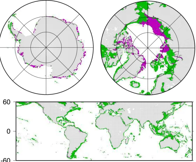
Antarctic zones could not be used due to discrepancies be-tween the ETOPO2 data set and the GMT coastline, and only 0.8% for the non-polar region. The Arctic, Antarctic, and non-polar regions represent, respectively, 24.1%, 1.8%, and 74.1% of the total coastal surface covered. Figure 1 shows these three zones with the non-available pixels on the Sea-WiFS composite image for the year 2000. Proximal coastal pixels are defined as pixels comprising a portion of the coast-line; all other coastal pixels are defined as distal.
2.2 SeaWiFS data
There are several levels of SeaWiFS data, two of which were used in the present paper. Level-2 data are geophysi-cal products such as the chlorophyll concentration or the dif-fuse attenuation coefficient, geographically referenced, and provided on an orbit per orbit (or scene by scene) basis at the spatial resolution of the satellite sensor. Level-3 data are averages of individual Level-2 data on a spatial grid (e.g., a 9 km global grid) and over a given time period (e.g., a month). Monthly and annual SeaWiFS Level-3 global com-posites were obtained from the NASA Goddard Space Flight Center DAAC, for the years 1998 to 2002. These data are organized on a 2048×4096 equirectangular projection with a constant latitude and longitude step (Campbell et al., 1995). The resolution at the equator is approximately 9 km. Three SeaWiFS-derived quantities were used: the upper-layer chlorophyll-a concentration (Csat) derived through the
-60
0
60
Fig. 1. The three geographical areas considered. Green and purple pixels are, respectively, pixels for which data are available or not on the SeaWiFS composite image for the year 2000.
water-leaving radiance at 555 nm, nLw(555), and the photo-synthetically available radiation at the sea surface, PAR(0+), computed following Frouin et al. (2003). A given bin of these Level-3 composites contains the arithmetic average of all in-dividual Level-2 1-km pixels that passed a series of exclusion criteria (Robinson et al., 2003).
2.3 Case 1 versus Case 2 waters
It is beyond the scope of this paper to review the criteria used to eliminate dubious data when generating a SeaWiFS Level-3 composite, except for discriminating the water type as ei-ther Case 1 or Case 2 (Morel and Prieur, 1977), as the latter type is well represented in coastal waters. The discrimina-tion between these two types is performed at the Level-2 in the SeaWiFS processing, yet it is not considered when gener-ating the Level-3 composites (B. Franz, personal communi-cation). Therefore, the average chlorophyll-a concentration in a given bin of a Level-3 composite may have been com-puted over any proportion of Case 1 and Case 2 waters. The
accuracy of Csat in Case 1 waters is claimed to be ±30%
whereas its is unknown in Case 2 waters. It is therefore not possible to estimate the accuracy of the chlorophyll product in coastal areas and, in turn, the accuracy of the diffuse at-tenuation coefficient. We apply an a posteriori determination of the water type based on the average Csatand nLw(555)
(see below), which is not based on specific algorithms for each water type (since no universal algorithm exists). This determination nevertheless provides an indication of bins of Case 2 water because, on average, the individual pixels in the bins were predominantly of the Case 2 type. Waters with a Csatvalue lower than 0.2 mg m−3are considered to be Case 1
(A. Morel, personal communication). When Csat is higher
than 0.2 mg m−3, the identification of turbid Case 2 waters is performed as in Morel and B´elanger (2006) by comparing the water reflectance at 555 nm (R(555)) to the maximum value it should have in Case 1 waters (Rlim(555)). Turbid
Case 2 waters are those for which R(555)>Rlim(555). To
the SeaWiFS product, is converted into R as follows (Morel and Gentili, 1996):
R(555) = nLw(555) × Q0(555) F0(555) × R0
(1) where F0(555) is the extra-terrestrial irradiance at 555 nm
(185.33 W m−2nm−1; Thuillier et al., 2003), Q
0(555) is the
chlorophyll-dependent Q-factor, i.e., the ratio of the upward irradiance to the upwelling radiance (Morel et al., 2002), and R0is a term which merges all reflection and refraction effects
at the air-sea interface (0.529). Since nLw is fully normal-ized (Morel and Gentili, 1996), its dependence on the view-ing angle and the sun zenith angle are removed so that both Qand R are taken for a nadir view and a sun at zenith (hence the “0” subscript).
2.4 Benthic irradiance
The diffuse attenuation coefficient for the downwelling irra-diance (KD) describes the exponential propagation of
spec-tral irradiance with depth in the water column. It deter-mines the amount of radiation reaching a given depth (Z) and whether light reaches the sea bottom:
KD =
−d[LN (Ed(λ, Z))]
dZ (2)
The spectral composition of the radiation is not considered in this work and only its integral value between 400 and 700 nm is used (i.e., the photosynthetically available radiation, PAR). The mean attenuation coefficient for PAR (KPAR) is
there-fore: KPAR=
−d[LN (PAR(Z))]
dZ (3)
The average value of KPAR over the euphotic zone was
de-termined as described by Morel (1988):
KPAR=0.121 × Csat0.428 (4)
This relationship has been established for open ocean Case 1 waters. However, the sole piece of information available in a given bin is the monthly average chlorophyll-a concen-tration (Csat). This average may include relatively accurate
chlorophyll-a concentrations determined in Case 1 waters and relatively inaccurate values determined in turbid Case 2 waters, the proportion of each being unknown. The impact on the computation of the diffuse attenuation coefficient is therefore unpredictable.
2.5 Comparison with KPARestimates derived from Secchi
disk depths
Secchi disk depths (Zsd) were extracted from the World
Ocean Database (Conkright et al., 1999). Zsd values are
included in the secondary header information, and include observations taken from the early 1900s through the 1990s.
Several studies have produced formula for converting Zsd (in m) to a light attenuation coefficient (KPAR). The
early formulae follow the general equation: KPAR=q/Zsd,
where q is an empirically determined constant. For Case 1 waters, the value of q was determined as 1.7 (Poole and Atkins, 1929; Idso and Gilbert, 1974), but for Case 2 waters q was determined to be around 1.4 (Gall, 1949). For this study, we used two formulae: (1) that of Holmes (1970), where KPAR=1.7/Zsd when Zsd<5 m and
KPAR=1.44 when Zsd>5 m; and (2) that of Weinberg (1976),
where KPAR=2.6/(Zsd+2.5)−0.048.
The Secchi-derived KPAR values were averaged for each
SeaWiFS gridcell. For grid cells with at least 10 Secchi disk depth observations and water depths less than 200 m, the av-erage secchi-derived KPARvalues were compared to the
av-erage SeaWiFS-derived KPARvalues (Fig. 2) for depths less
than 200 m. The SeaWiFS-derived KPARvalues were
consis-tently less than those derived from the Secchi disk depths, al-though use of the Weinberg (1976) formula produced slightly better correlations with the SeaWiFS data. Correlations were best in Case 2 waters, and decreased at higher KPARvalues.
2.6 Compilation of data
The minimum light requirements (Emin) of the major groups
of photosynthetic organisms were compiled from the liter-ature. The annual average irradiance at depth (Ez) is not
often reported but KPAR or the percent surface irradiance
(%E0) often is. In such cases, Emin was estimated from
KPARor %E0using the average daily surface irradiance
pro-vided by SeaWiFS. Irradiance data expressed in energy units were converted to molar units using a conversion factor of 2.5×10¹⁸ quanta s−1watt−1 or 4.2 µmol photons m−2s−1 watt−1(Morel and Smith, 1974).
3 Results
This section is devoted to the analysis of the SeaWiFS data. The compilation of literature data on the constraints of light availability on the major primary producers and NCP is pre-sented in the discussion section.
The Antarctic region is poorly covered by the SeaWiFS sensor due to limitations of the algorithms against sun-zenith angles, and to the presence of ice. Only 36% of the coastal zone is available in the annual images, and 26% are available in the best monthly image (February 2003). As this region only represents 1.8% of the surface area of the world coastal zone, it was not considered further in this analysis. Temporal variations for the Arctic and non-polar regions are shown in Fig. 3. Other data are summarized in Tables 1 and 2. Appen-dices A and B provide the gridded data of the geographical distribution of Case 1 and Case 2 waters as well as of benthic irradiance, respectively.
Table 1. Surface area and average depth of the various pixel classes. Ez=1% is the level at which benthic irradiance equals 1% of surface
irradiance. Available pixels are those for which Csat, nLw(555) and PAR are available for analysis. Proximal coastal pixels are defined as
pixels comprising a portion of the coastline; all other coastal pixels are defined as distal.
Arctic Non-polar
Monthly images Monthly images
(June–October)
Min Max Mean Min Max Mean
Available pixels/total number of pixels 0.20 0.60 0.39 0.68 0.90 0.81
Average depth available pixels (m) 74 87 80 67 71 69
Case 1 pixels/available pixels 0.58 0.72 0.66 0.46 0.65 0.55
Average depth Case 1 pixels (m) 86 99 93 80 86 83
Case 2 pixels/available pixels 0.28 0.42 0.34 0.35 0.54 0.45
Average depth Case 2 pixels 43 70 55 44 57 52
Pixels Ez=1%/available pixels 0.20 0.29 0.25 0.35 0.41 0.37
Average depth pixels Ez=1% (m) 14 18 16 21 24 22
Proximal pixels/available pixels 0.07 0.10 0.08 0.19 0.47 0.30
Average depth proximal pixels (m) 25 29 28 19 23 22
Distal pixels/available pixels 0.90 0.93 0.92 0.53 0.81 0.70
Average depth distal pixels (m) 70 77 73 43 74 63
Annual images Annual images
Min Max Mean Min Max Mean
Available pixels/total number of pixels 0.67 0.68 0.68 0.96 0.96 0.96
Average depth available pixels (m) 73.8 74.4 74 67.7 67.9 67.9
Case 1 pixels/available pixels 0.65 0.69 0.67 0.53 0.57 0.55
Average depth Case 1 pixels (m) 89.2 91.4 90.4 84.5 86.1 85.3
Case 2 pixels/available pixels 0.31 0.35 0.33 0.43 0.47 0.45
Average depth Case 2 pixels (m) 39.4 45.4 41.5 45.1 47.7 46.8
Pixels Ez=1%/available pixels 0.27 0.30 0.28 0.35 0.36 0.36
Average depth pixels Ez=1% (m) 14.5 16.1 15.2 19.5 19.9 19.7
Proximal pixels/available pixels 0.08 0.09 0.08 0.79 0.80 0.80
Average depth proximal pixels (m) 26.5 27.7 27.3 19.4 19.7 19.5
Distal pixels/available pixels 0.91 0.92 0.92 0.20 0.21 0.20
Average depth distal pixels (m) 74.9 75.8 75.5 33.5 34.5 33.6
Table 2. Surface area (S) and average depth (Z) of coastal waters of different optical characteristics.
Arctic Non-polar S (106km2) S(%) Z(m) S (106km2) S(%) Z(m) Coastal zone 6.13 100 73.3 18.82 100 66 Monthly images Case 1 1.6 26.2 92.8 8.47 45 83 Case 2 0.81 13.2 54.6 6.76 35.9 52 Cases 1 and 2 2.41 39.4 80 15.23 80.9 69 Annual images Case 1 2.75 44.9 90.4 9.93 52.7 85 Case 2 1.39 22.6 41.5 8.19 43.5 47 Cases 1 and 2 4.14 67.5 74.1 18.11 96.2 68
0.0 0.5 0.0 0.5 Secchi KPAR (m -1) 0.0 0.1 0.2 0.3 0.4 0.5 0.0 0.1 0.2 0.3 0.4 0.5 All data A 0.0 0.5 0.0 0.5 Secchi KPAR (m -1) 0.0 0.1 0.2 0.3 0.4 0.5 0.0 0.1 0.2 0.3 0.4 0.5 Case 1 B 0.0 0.5 SeaWiFS KPAR (m -1 ) 0.0 0.5 Secchi KPAR (m -1) 0.0 0.1 0.2 0.3 0.4 0.5 0.0 0.1 0.2 0.3 0.4 0.5 Case 2 C
Fig. 2. KPAR values derived from Secchi disk depth data
us-ing the formulation of Weinberg (1976) versus KPAR derived
from SeaWiFS data. The 1:1 line is shown. Model II
regres-sions are: y=−0.023+1.43×x (N =3424; r=0.76) for all data,
y=0.022+0.87×x (N =2126; r=0.51) for Case 1 waters, and
Y =0.002+1.68×x (N =467; r=0.73) for Case 2 waters. N is the
number of data and r is the Pearson correlation coefficient. The slopes of the geometric regression forced through the origin are 1.25, 1.05 and 1.7, respectively for all data, Case 1 waters and Case 2 waters. Note that correlations are not shown for locations where waters varied seasonally between Case 1 and Case 2 in the SeaWiFS calculations.
3.1 Arctic region
Data availability vary greatly with season in the Arctic re-gion. In monthly images, the fraction of the coastal zone available for analysis ranged from 0 in winter (November, December and January) to less than 0.10 in February, March, April and May; these 7 months were therefore not further considered. The fraction of data available of the remaining 5 months ranges from 0.20 to 0.60 and is about 0.68 on an-nual images (Tables 1). From these data were calculated the fractions (of the available coastal zone) of: Case 1 waters (f1), Case 2 waters (f2), and the fraction of the coastal ocean
where the bottom irradiance is more than 1% of the incident surface irradiance (f1%). On average, f1=0.66 and f2=0.34
on both annual and mean monthly images, f1%=0.25 in
monthly images and 0.28 in annual images, and 92% of the missing pixels are distal. Of course, the variability is greater on monthly images but, on average, the results are similar in monthly and annual images.
3.2 Non-polar region
In non-polar regions, the fraction of the total coastal zone surface area available for analysis was 0.96 in the annually-averaged images, and varied from 0.68 to 0.90 in the monthly images. On average, f1=0.55 and f2=0.45 on both monthly
and annual images, and f1%=0.37 (monthly) or 0.36
(an-nual). Aside from the variability, the main difference be-tween monthly and annual images is the proximal/distal ratio of non-available pixels. The proximal/distal ratio is 0.30/0.70 on monthly images and 0.80/0.20 on annual images. This is because distal pixels, which are mainly affected by cloud cover on monthly images, are available on annual images (where missing distal pixels represent only 1% of the total surface).
3.3 Surface area as a function of incident light
Let us define the cumulative function P : given an irradiance level on the sea floor Ez, P is the percentage of the surface
of the coastal zone receiving an irradiance greater than Ez
(in mol photons m−2d−1). This percentage was calculated for each of the monthly and annual images. The average an-nual function (Pa, the mean of the annual functions) was
cal-culated, as well as the average monthly P -function for each month (12 for the non-polar region and 5 for the Arctic re-gion, as explained in Sect. 3.1). For example, Pjune is the
mean of the P -functions calculated for all June images be-tween 1998 and 2003. Finally, the Pm function was
con-structed as the mean of the monthly P -functions. In the Arc-tic region, the Paand Pmfunctions are different because
an-nual images in this region, where data are not available dur-ing 7 months, are strongly biased. In the non-polar region, the Pa and Pmfunctions provide similar percent surface
0
20
60
100
Surface area (% total)
1998 2000 2002 Time available data z<z1% Case 1 Case 2 1998 2000 2002 % of unavailable pixels 0 20 40 60 80 Time proximal distal 0 20 60 100
Surface area (% total)
1998 2000 2002 Time available data z<z1% Case 1 Case 2 1998 2000 2002 % of unavailable pixels 0 20 40 60 80 Time proximal distal
A: Arctic
Fig. 3. Monthly and annual changes in the surface area of the SeaWiFS pixels available (i.e. for which Csat, nLw(555) and PAR are available
for analysis), Case 1 and Case 2 pixels, and of the geographical zone where irradiance is higher than 1% of surface irradiance (Z1%) in the
Arctic and non-polar regions. The percent contribution of the proximal and distal pixels to the total number of pixels not available is also shown. Proximal coastal pixels are defined as pixels comprising a portion of the coastline; all other coastal pixels are defined as distal.
and maximum values, and a relative error of less than 4% be-tween Paand Pmfor Ez<10 mol photons m−2d−1). Pmis
therefore used for the rest of this study. Figure 4 shows the Pmfunctions. The surface area receiving a certain irradiance
threshold is larger for Case 2 than for Case 1 waters because the former are shallower than the later (e.g. 52 vs. 83 m in the non-polar region; Table 1).
4 Discussion
Coastal and offshore waters have been classified into several types according to their optical characteristics (e.g., Jerlov, 1977; Morel and Prieur, 1977; Pelevin and Rutkovskaya, 1977). Several local and regional distributions of these water types are available but their large scale geographical distribu-tions are unknown. This study is the first attempt to describe the distribution of two water types in the coastal ocean, with optical characteristics dominated (Case 2) or not (Case 1) by allochthonous CDOM and suspended solids. In this sec-tion, the validity of the assumptions involved in the method used and the resulting uncertainties are analyzed. The geo-graphical distributions of Case 1 and Case 2 waters are then discussed, the irradiance reaching the bottom of the coastal ocean estimated, and, together with the light requirement of
the major benthic primary producers, is used to estimate the surface area of the coastal ocean where benthic primary pro-duction can proceed. These areas are broken down as polar vs. non-polar, and Case 1 vs. Case 2.
4.1 Distribution of benthic irradiance and assumptions in-volved
Pixels not available for analysis have three origins: (1) data acquisition was not performed because the area was not cov-ered by SeaWiFS (high latitude), (2) data were collected but subsequently eliminated either due to high reflectance from adjacent land or to high turbidity, and (3) cloud cover pre-vented acquisition of useful data. These three sources vary, some of them considerably, with season. This is consis-tent with many observations that specific geographical loca-tions on the continental shelf belong to different optical water types depending on the season (Højerslev and Aarup, 2002). However, only 12% of the surface area of the coastal ocean is missing on annual images and it is mostly represented by distal pixels (with an average depth of 73 m), most of which probably do not experience light penetration to the bottom. Only 3% of the missing proximal pixels (average depth of 22 m) can potentially receive irradiance at the bottom. An-other possible drawback of using annual images is that some
Irradiance (mol photons m−2d−1) Surface area (%) 0 20 40 60 80 0 20 40 60 80 10 1 0.1 0.01 Case 1 Case 2
Case 1 and Case 2
Arctic
Irradiance (mol photons m−2d−1)
Surface area (%) 0 20 40 60 80 0 20 40 60 80 10 1 0.1 0.01 Case 1 Case 2
Case 1 and Case 2
Non polar
Fig. 4. Cumulative surface area of the sea floor (S) receiving irradiance above a prescribed threshold (Ez). Data are expressed in percent of
the surface area for which information is available (6 126 726 and 18 821 140 km2, respectively for the Arctic and non-polar regions). For
example, in the non-polar region, about 20% of the surface area overlain by Case 1 waters receives at least 1 mol photons m−2d−1. The
shaded zone depicts the range all monthly P -functions for case 1 and case 2 waters. The solid lines correspond to the annual functions
calculated as the average of the monthly functions (Pm). Note that data for the Arctic are based on the five months of the year when light
levels were within the detection limits of the SeaWiFS sensor; i.e., only summer months were included (see Sect. 3.1). For this region, to
convert the daily irradiance value (mol photons m−2d−1) to an annual irradiance value (mol photons m−2y−1), one must multiply the daily
value by (5/12)×365 d y−1. The polynomial equations of the lines shown are:
Arctic Case 1: S=10.13−9.15 log10(Ez)+2.12 log210(Ez)+0.31 log310(Ez);
Arctic Case 2: S=27.56−22.26 log10(Ez)+0.25 log210(Ez)+1.48 log310(Ez);
Arctic Case 1 and Case 2: S=15.99−13.56 log10(Ez)+1.49 log210(Ez)+0.70 log310(Ez);
non-polar Case 1: S=21.07−14.64 log10(Ez)+1.97 log210(Ez)+0.83 log310(Ez);
non-polar Case 2: S=40.29−22.03 log10(Ez)−0.86 log210(Ez)+0.97 log310(Ez);
non-polar Case 1 and Case 2: S=29.61−17.92 log10(Ez)+0.72 log210(Ez)+0.90 log310(Ez).
areas have only been sampled a few times over the period of one year. This introduces a bias in areas where light pene-tration varies with season, particularly in high-latitude envi-ronments. In the Arctic, for example, light levels could only be calculated for the five summer months, and we calculated the annual average light penetration based only on those five months. This provides a more realistic value of light at the surface and its depth of penetration (including the dark win-ter months would have grossly underestimated the percent
surface area that can support photosynthesis), but the limita-tion must be taken into account when extrapolating the data to a full year (that is, significant photosynthesis only occurs on the Arctic shelf for five months). Parameters other than day length change seasonally, such as river discharge, wave height and resulting sediment resuspension, and water col-umn stratification (R. Jahnke, personal communication).
The overall comparison of the SeaWiFS chlorophyll data with field measurements is quite remarkable with an r2 of
0.76 (Gregg and Casey, 2004). When data are split into open ocean and coastal waters (using the 200 m depth con-tour), the correlation is significantly lower in the coastal ocean than in the open ocean (r2 of 0.60 vs. 0.72). Ac-cording to Gregg and Casey (2004), there are more than ten impediments to retrieval of accurate water column chloro-phyll from ocean color remote sensing. Among them, the presence of allochthonous chromophoric dissolved organic matter (CDOM) and suspended sediments mostly apply to coastal waters. The regional analyses that they carried out show that the standard SeaWiFS algorithm overestimates the chlorophyll concentration in coastal region. We have esti-mated that 38% of the ratios SeaWiFS:in situ chlorophyll are below 1 while 62% are above 1. In addition the the water-column impediments listed by Gregg and Casey (2004), sed-iment resuspension near the sea floor can greatly reduce ben-thic irradiance (R. Jahnke, personal communication). It was not taken into account in the present study but more benthic irradiance data would be needed to assess its importance on a global scale.
The nearly global scope of the present analysis does not capture the large spatial and temporal variability of the light field in the coastal ocean. For example, changes in the optical properties of the water column occur within scales of a few 100 m and daily irradiance can change by up to one order of magnitude or more in a coastal turbid environment. Anthony et al. (2004) identified four key factors which affect temporal changes of irradiance: (1) the seasonal pattern of daily sur-face irradiance, (2) cloudiness, (3) light transmission in the water column which depends on turbidity and (4) tides.
According to the criteria used, more than half (55%) of the coastal ocean has optical characteristics of Case 1 waters (Ta-ble 2), and are hence relatively unaffected by allochthonous CDOM and suspended solids. Another unexpected outcome of this study is that Case 2 waters are not preferentially tributed close to shore. A large fraction (43%) of areas dis-tant from shore are affected by allochthonous CDOM and suspended solids, probably corresponding to river plumes and relatively shallow areas influenced by sediment resus-pension or upwelling.
The euphotic zone typically exhibits an excess of gross primary production over community respiration, hence net community production is positive. Its lower limit is often ar-bitrarily set at 1% of surface irradiance. According to our analysis (Table 1), 25 and 37% of the Arctic and non-polar coastal zone receive more than this level (34% for these two regions combined). Nelson et al. (1999) reported that bottom irradiance is often 4 to 8% of surface irradiance over much of the South Atlantic Bight, and exceeds 10% of surface ir-radiance on occasion. Jahnke et al. (2000) estimated that the area-weighted annual average light flux to the sea floor of the Southeastern US continental shelf is 5.4% of the surface irradiance (or 1.8 mol photons m−2d−1).
Expressing light requirements for benthic primary produc-tion in percent of surface irradiance, however, is biologically
meaningless (L¨uning and Dring, 1979). The distribution of photosynthetic organisms and the metabolic performances of photosynthetic communities are controlled by absolute irra-diance levels, or compensation irrairra-diance (see below). Per-cent of surface irradiance does not translate into absolute ir-radiance because the surface irir-radiance itself varies consider-ably with latitude and cloud cover (e.g., Kl¨oser et al., 1993). Banse (2004) recently advocated the use of absolute rather than percent of incident irradiance for phytoplankton com-munities, pointing out that the 1%-depth for moonlight is about the same as the 1%-depth for sunlight. The analysis that follows is therefore based on absolute rather than rela-tive irradiance.
4.2 Distribution of major primary producers and net ecosystem metabolism
In this section, we compile data on the constraint of light availability on the major benthic primary producers and on net community production. Then, the data are combined with the irradiance data derived in Sect. 3.1 to produce estimates of the surface area where (1) light does not limit the distribu-tion of primary producers and (2) net community producdistribu-tion (the balance between gross primary production and commu-nity respiration) is positive.
4.2.1 Metrics of light requirements
Benthic primary producers, including prokaryotes, plants, and animals living in symbiosis with algae (e.g., zooxanthel-late corals), rely on irradiance to proceed with photosynthe-sis. The dependence of benthic primary production on irra-diance can be defined by three distinct compensation irradi-ances:
– Compensation irradiance for photosynthesis (Ecphot.):
This is the irradiance at which net photosynthesis is 0 (the rates of gross photosynthesis and autotrophic res-piration are equal). Instantaneous Ecphot. is typically
inferred from experimental photosynthesis-irradiance curves in laboratory of field incubations over time spans of less than 24 h, sometimes over seconds. The daily
Ecphot. is defined for a period of 24 h and is the daily
irradiance below which daily net photosynthesis is 0. It is not often reported in the literature.
– Compensation irradiance for growth (Ecgrowth; sensu
Markager and Sand-Jensen, 1994): This is the irradi-ance at which gross primary production balirradi-ances the carbon losses (respiration, herbivory, exudation of dis-solved organic carbon, and reproduction) for a partic-ular organism. Ecgrowth is inferred from long-term
growth-irradiance experiments (Markager and Sand-Jensen, 1994) or, empirically as the irradiance at the depth limit of the distribution of benthic primary pro-ducers (e.g. Appendix 1 in Duarte, 1991). For benthic
0 500 1000 1500 −40 −20 0 20 40 60 80 100
Instantaneous benthic irradiance (µµmol m−2 s−1)
Net production (arbitrary units)
Organism Community A 0 5 10 15 20 −0.5 0.0 0.5 1.0 1.5
Time of the day (h)
Net production (arbitrary units)
Organism Community B 0 10 20 30 40 50 0 5 10 15
Daily benthic irradiance (Ez in mol m−2 d−1)
Daily
Ec
(continuous line; mol
m −2 d −1) 0 5 10 15 Instantaneous Ec
(dashed line; mol
m −2 d −1 ) Organism Community Ec = Ez C
Fig. 5. Arbitrary P −E curve (A), diel change of net pri-mary (insets) and community production (B) and changes in
daily Ec as a function of daily irradiance (C) for
photosyn-thetic organisms and communities. The primary production of
an organism was calculated using the hyperbolic tangent function npp=gppmax×tanh(Ez/Ek)+rawhere: npp is the rate of net
pri-mary production, gppmax is the maximum rate of gross primary
production (set at 100), Ezis the benthic irradiance, Ek is the
ir-radiance at which the initial slope of the P −E curve intersects the
horizontal asymptote (set at 50 µmol photons m−2s−1) and rais
the rate of dark respiration of the autotrophs (set at −20). Ezand
Ek are in µmol photons m−2s−1. The diel change in irradiance
was modeled using a sine curve and using a photoperiod of 12 h dark and 12 h light. The rate of net community production was calculated assuming that the rates of dark respiration of the
het-erotrophs and autotrophs are equal. rawas therefore simply added
to the npp of the organism. In this generic example, the
instan-taneous Ecphot. (i.e. for the organism) and Eccomm.(i.e. for the
community) are, respectively, 101 and 212 µmol photons m−2s−1
(panels A and B). In panel (C), daily Ec(continuous lines) is twice
the instantaneous Ec(dashed line) and the shaded area indicates the
range of daily Ec for communities. This area is enclosed within
an upper line which assumes no photoacclimation and a lower line which assumes a photoacclimation parallel to the one reported for individual organisms. The thick blue line shows the range of daily
compensation irradiance. Irradiance in µmol photons m−2d−1is
calculated using the relationship 0.0432 × irradiance (in µmol
pho-tons m−2s−1) assuming a photoperiod of 12 h dark and 12 h light.
organisms, Ecgrowth also integrates the light
require-ments over long periods of time, effectively smoothing out seasonal changes in irradiance. Here one assumes that light attenuation with depth is the only factor limit-ing the vertical distribution, although other factors limit the colonization depths of benthic primary producers (e.g., terracing, thermocline, competition, etc.).
– Compensation irradiance for community metabolism
(Eccomm.): This is the irradiance at which gross
com-munity primary production (GPP) balances respiratory carbon losses (R) for the entire community. Instanta-neous Eccomm.is typically inferred from experimental
photosynthesis-irradiance curves over time spans of less than 24 h. The daily Eccomm.is derived from concurrent
measurements of daily irradiance and daily net commu-nity production (NCP) at different depths. The use of shading experiments on communities at a single depth (e.g. Gacia et al., 2005) are useful in investigations of short-term (a few weeks) photoacclimation but do not provide useful information on metabolic performances as a function of depth because they do not account for depth-related changes in the community composition. Additionally, such experiments must be relatively long (up to a few months) in order to ascertain that the com-munity is acclimated to the new light field.
These three compensation irradiances have different mean-ing, availability, and usefulness in the context of this paper.
Ecphot. is by far the most often reported measure of
com-pensation irradiance while Eccomm. is the least often
mea-sured, being limited to a few experiments carried out mostly on shallow water communities. Ecphot.is an important
phys-iological trait, but does not have a direct translation into the distribution and long-term production of benthic organisms. It approximates Ecgrowth only when measurements are
ob-tained from individuals collected close to the depth limit of a particular species or acclimated at an irradiance close to that found at the depth limit (Markager and Sand-Jensen, 1992). These conditions are not frequently met. Ecgrowth,
for which there is a reasonable empirical basis, is the relevant parameter for estimating the areal extent of benthic primary producers (the area receiving irradiances ≥Ecgrowth).
Ben-thic communities growing at irradiances close to Ecgrowth
are unlikely to exhibit a positive NCP. This is because R, which is often sizeable relative to GPP, should exceed GPP
at Ecgrowth, rendering deep photosynthesizing communities
heterotrophic with respect to carbon (i.e., dependent on in-puts of organic carbon from adjacent systems). Eccomm.
rep-resents the threshold irradiance above which benthic com-munities are autotrophic and can contribute to net production of organic carbon in coastal ecosystems. Note that net pri-mary production of the autotrophs can be significant below this threshold, even though the community is heterotrophic.
We will focus on Ecgrowth and Eccomm. as the
thresholds for benthic communities. These thresholds respectively delineate the deepest extent of benthic primary producers and the depth over which benthic communities act as net sources of organic carbon to coastal ecosystems. Figure 5 illustrates the relationship between Ecphot. and
Eccomm.and their changes with irradiance. Three important
observations are apparent in this figure. First, instantaneous
Eccomm. should be higher than instantaneous Ecphot.
(Figs. 5a and c). It should also occur later in the morning and earlier in the afternoon (Fig. 5b) because communities include heterotrophs as well as autotrophs, which increases respiration relative to primary production and thus raises the compensation irradiance. Second, instantaneous Ecphot.
of organisms generally decreases with decreasing benthic irradiance due to photoacclimation: low-light adapted specimens therefore have less light requirements than high-light adapted specimens (Fig. 5c). Third, the slope of the relationship Ecversus Ezis lower for communities than
for organisms because the ratio of autotrophs to heterotrophs decreases with decreasing irradiance.
For ecosystems such as coral reefs, the precise photoac-climation function is unknown because Eccomm. data are
reported as instantaneous values obtained on shallow-water communities whereas, as outlined above, daily values at depths are required to estimate the surface area of the coastal ocean which receives enough light to contribute to net pri-mary production. The photoacclimation function can be bracketed by an upper bound which assumes no photoaccli-mation and a lower bound which assumes that photoacclima-tion of communities is similar to that observed in the main photosynthetic organism of the community. The true func-tion lies in the light blue area shown in Fig. 5c).
4.2.2 Review of the light requirements of benthic primary producers
The maximum depth of distribution of primary producers, which represents an estimate of Ecgrowth, ranges from 90 to
285 m corresponding to 11 to 0.0005% of incident surface irradiance (Table 3). These depths demonstrate the outstand-ing photoadaptative capabilities of some primary producers but are not very useful for estimating their global depth dis-tribution. Logically, benthic primary producers occur most deeply in exceptionally clear waters, in accordance with the negative relationship between the depth limit and water trans-parency (e.g. Duarte, 1991, for seagrasses). Moreover, ben-thic primary producers occur in very low abundance at these depths, where their contribution to primary production is negligible. The light requirements of the major benthic pri-mary producers are reviewed below, but we first address the special case of organisms living in polar regions.
Special consideration for polar regions
Polar regions are the most difficult to address due to scant information on benthic irradiance along the Antarctic coast (see Sect. 3), vertical distribution of primary producers, and acclimation processes other than photoacclimation. Estimat-ing light penetration on a large spatial scale is difficult at high latitudes because of the poor coverage by SeaWiFS (Sect. 4.1) and the considerable seasonal change in light ab-sorption by ice and snow covers, and sub-ice platelets. How-ever, there are local estimates of light penetration. For ex-ample, Robinson et al. (1995) reported that approximately 0.05% of the irradiance incident on the sea ice (about 2 m thick) surface at noon or 0.2 to 0.6 µmol photons m−2s−1 reaches the sea floor at 23 m depth in McMurdo Sound, Antarctica. Borum et al. (2002) provided estimates of the cumulated annual benthic irradiance in a high-arctic fjord of NE Greenland covered by ice for about 10 months a year: 234, 96 and 40 mol photons m−2year−1at 10, 15 and 20 m depth, respectively. Schwarz et al. (2003) estimated that an-nual irradiance at Cape Evans (77◦380S) ranges from 111.6 to 17.7 mol photons m−2year−1, respectively at 10 and 30 m depth. It must also be noted that coastal waters can be clear under the ice; a KPARvalue of 0.09 m−1was reported in the
Ross Sea (Schwarz et al., 2003).
The cumulated annual irradiance at depth probably con-trols the depth distribution of photosynthetic organisms. The seasonal depth of light penetration exhibits dramatic seasonal changes at high latitudes: the total insolation in summer may actually exceed that of lower latitudes (because of longer day length) but, due to higher zenith angles, more of the light is reflected off the surface rather than penetrating the air-sea in-terface. Some organisms may require some daily minimum irradiance to survive; that is, their bottom limit of distribu-tion is limited by winter time irradiance. Others are known to suspend growth during winter darkness, aided by the re-duced carbon expenditure as reflected in lower rates of respi-ration in colder waters. At 20 m, the depth limit for the alga
Laminaria saccharina in an Arctic Greenland fjord, annual
irradiance is 40 mol photons m−2or about 0.7% of surface irradiance (Borum et al., 2002). The net carbon balance is negative during most of the ice covered period but the sum-mer primary production is large enough to maintain a posi-tive annual carbon balance (GPP/R=1.2). Despite extended periods of extreme light limitation, and because of strong photoacclimation processes, the light requirement at this site is only slightly lower than that of other cold-water laminari-ales (e.g., L¨uning and Dring, 1979). This suggests that light limitation for this group of macroalgae, and possibly others, should therefore be considered on an yearly basis.
Saprotrophy, the ability to assimilate dissolved organic substrates, is another acclimation process that can support normally photosynthetic organisms during periods of low ir-radiance. Antarctic benthic diatoms, for example, can be saprotrophic. This ability could also support heterotrophic
Table 3. Deepest known benthic primary producers. Note that data for microalgae may be the result of downslope transport, although this possibility was ruled out by Cahoon (1986).
Seagrasses Macroalgae Microalgae Corals
Reference Den Hartog (1970) Littler et al. (1985) Cahoon (1986) Maragos and Jokiel (1986)
Deepest record (m) 90 268 285 165
% surface irradiance 11 0.0005 0.1 0.02
Ecgrowth(mol photons m−2d−1) 5 0.0002 0.04 0.009 (a)
(a) KPARfrom Agegian and Abbott (1985)
growth of microphythobenthic algae during the aphotic polar winter (Rivkin and Putt, 1988).
The depth limits of Antarctic macroalgae have been com-piled by Kl¨oser et al. (1993). Benthic photosynthesis occurs despite very low light levels due to periods of darkness of up to four months, and cloud, ice and snow covers. Coralline algae have low light requirements, can sustain prolonged pe-riods of darkness, and seem to be well distributed at high latitudes (Schwarz et al., 2003). Brown algae have light re-quirements as low as 31 mol photons m−2year−1(Wiencke, 1990, in Schwarz et al., 2003).
Surface area potentially available for benthic primary pro-ducers
Here we combine estimates of the irradiance reaching the bottom of the coastal ocean derived in Sect. 3.3 with esti-mates of Ecgrowthto provide the maximum extent of the area
of distribution of different benthic organisms. The limita-tions related to the use of SeaWiFS data to estimate the ir-radiance reaching the sea floor are described in Sect. 4.1. There are also biological and sedimentological sources of uncertainty. The method of estimating benthic irradiance as-sumes that there is no shading from other erect organisms nor epibionts. The effects of backscaterring within the sediment, which can result in a 50% increase of the light exposure of some microphytobenthic communities (K¨uhl and Jørgensen, 1992), are also neglected. Finally, tidal effects were ignored, which in areas subject to large tidal amplitude, can induce hourly, daily and seasonal variations in light penetration by altering the height of the water column and turbidity (e.g., Dring and L¨uning, 1994). Data on both the maximum depth of occurrence of species and the irradiance at this depth were compiled from the literature to determine the surface area where benthic primary producers are not light limited. Often the benthic irradiance was not reported but either the attenu-ation coefficient or the percent light penetrattenu-ation was (some-times in another paper); in this case, the benthic irradiance was estimated by combining this value with the surface PAR value from SeaWiFS.
Bacteria and Archaea
Photosynthetic Bacteria and Archaea are very diverse, both taxonomically and functionally as they utilize the three known types of photosynthesis (Karl, 2002). Oxygenic pho-tosynthesis generates oxygen as a by-product whereas aero-bic anoxygenic and anaeroaero-bic anoxygenic photosynthesis do not. Their importance is likely minor in terms of global ben-thic primary production. The very poor knowledge on the depth distribution and light requirements of Bacteria and Ar-chaea prevents any attempt to delineate the extent of their ge-ographic distribution. It is, however, worth noting that some of them have developed extremely efficient mechanisms to acclimatize to light levels as low as 0.0005% of surface ir-radiance (or 0.003 µmol photons m−2s−1; Overmann et al.,
1992).
Seagrasses
Seagrasses are flowering plants that grow on various soft sub-strata along the shores of all continents, except Antarctica, up to 75◦N. They colonize areas with suitable sediments down to 10.8% of surface irradiance (Duarte, 1991) and the deepest depth of colonization is 90 m in the Dry Tortugas (Table 3; Den Hartog, 1970). Duarte (1991) reviewed literature data on seagrass depth distribution and light attenuation and de-rived the following relationship between the maximum colo-nization depth (Zc, in m) and the light attenuation coefficient
(KPAR, in m−1):
LN (Zc) =0.26 − 1.07 × LN (KPAR) (5)
A few additional data were added to Duarte’s compilation. The data on Zostera marina produced by Nielsen et al. (2002) were not used because the geographical location of the stations was not provided. However, the distribution of this species in Danish waters is very well covered in our data set (available in Appendix C) from the 20 stations reported by Nielsen et al. (1989). The maximum depth of distribution of seagrasses ranges from 0.7 to 50 m, with a median value of 4.4 m. The minimum light requirement varies widely across species (range of median: 0.06 to 14.1 mol photons m−2d−1; Table 4). The overall median of the minimum light require-ment is 5.1 mol photons m−2d−1. About 19% and 38% of
Table 4. Minimum light requirements (mol photons m−2d−1) of seagrasses. The complete data set is available in Appendix C.
Species Number of data Range Mean Median
Cymodocea nodosa 2 0.1–0.1 0.1 0.1 Halophila decipiens 1 – 3.8 3.8 Halophila engelmannii 1 – 10.2 10.2 Halophila stipulacea 1 – 0.2 0.2 Heterozostera tasmanica 9 0.7–8.2 2.9 1.7 Posidonia angustifolia 2 2.4–10.1 6.2 6.2 Posidonia coriacea 1 – 3.2 3.2 Posidonia oceanica 2 0.1–2.8 1.4 1.4 Posidonia ostenfeldii 1 – 10.1 10.1 Posidonia sinuosa 1 – 10.1 10.1 Ruppia sp. 1 – 3.3 3.3 Syringodium filiforme 3 0.2–8.3 5.3 7.5 Thalassia testudinum 15 0.2–14.1 8.6 8.5 Thalassodendron ciliatum 3 1–4.4 2.2 1.3 Zostera marina 45 1.2–12.6 6.0 5.4 All 88 0.06–14.1 5.8 5.1
Table 5. Percent surface area where irradiance does not limit the distribution of photosynthetic organisms. Data are expressed relative to the
surface area for which information is available: 18 821 140 and 6 126 726 km2, respectively for the non-polar and Arctic regions. Data are
not reported in the Arctic region for seagrasses nor for reef corals where these groups are not present.
Non-polar region Arctic region
Organism Case 1 Case 2 Cases 1 and 2 Case 1 Case 2 Cases 1 and 2
Seagrasses 19 38 28 – – –
Macroalgae
– Filamentous and slightly corticated filamentous 32 55 42 17 43 26
– Corticated foliose, corticated and foliose 37 61 47 21 49 30
– Leathery and articulated calcareous 43 67 54 26 55 36
– Crustose 60 72 66 48 57 51
Microphytobenthos 27 49 37 14 36 22
Scleractinian corals 33 56 43 – – –
the surface area respectively covered by Case 1 and Case 2 waters in non-polar regions receive at least this irradiance level (Table 5). Globally, seagrasses are not light-limited in only 28% of the non-polar region (5.19×10⁶km2). This sur-face area is about 9 times larger than the estimated poten-tial area covered by seagrasse of 0.5 to 0.6×10⁶km2(Duarte and Chiscano, 1999; Green and Short, 2003), which were also based on considerations of the potential suitable habitat, and 35 times larger than the documented seagrass extension (about 0.15×10⁶km2; Green and Short, 2003). The estimate produced here represents an upper limit which needs be cor-rected for the area occupied by other benthic communities (coral reefs and macroalgae) and unsuitable substrate, such as rock or highly mobile sediments. Yet, it suggests that pre-vious estimates of the seagrass extension in the coastal zone were too conservative and that the actual area may be much larger than hitherto believed.
Although the scope of the present paper is global, data on light penetration and requirements are useful at the re-gional scale too. A good case study is the distribution of seagrasses in Australia. It also provides an opportu-nity for validation purposes and to highlight that parame-ters other than irradiance also control the distribution of ben-thic organisms. The Commonwealth Scientific and Indus-trial Research Organisation (CSIRO) compiled data on the distribution of seagrasses along the Australian coastline in 1996 (http://www.marine.csiro.au/nddq/ndd search.Browse Citation?txtSession=246). The potential distribution of sea-grasses in this region, estimated as the area where the ben-thos receives more than 5.1 mol photons m−2d−1, is much larger than the distribution estimated by CSIRO (Fig. 7). A large patch, also captured in the present study, is reported by CSIRO in the Torres Strait. The discrepancy is largest along the northern and northeastern coasts and can be explained
Table 6. Minimum light requirements (mol photons m−2d−1) of the major macroalgal functional groups defined by Steneck (1988) and Steneck and Dethier (1994). The complete data set is available in Appendix D.
Functional group Number of data Range Mean 1st decile Median
Filamentous (group 2) 7 0.1082–2.63 1.40 0.12 1.56
1.63
Slightly corticated filamentous (group 2.5) 5 0.9289–2.63 1.95 1.18 2.03
Corticated foliose (group 3.5) 29 0.0483–2.49 0.87 0.11 0.88
0.85
Corticated (group 4) 29 0.0317–2.63 0.93 0.1 0.81
Foliose (group 3) 4 0.0842–0.25 0.13 0.09 0.10
0.28
Leathery (group 5) 22 0.0277–1.53 0.50 0.06 0.31
Articulated calcareous (group 6) 16 0.011–2.92 0.65 0.04 0.19
Crustose (group 7) 28 0.0001–5.0 0.42 0.001 0.02 0.01
Undefined 22 0.0019–4.42 1.16 0.37 0.44 0.44
All 162 0.0001–5.0 0.81 0.019 0.31 –
by three reasons. First, several parameters beside irradiance limit the distribution of seagrasses (e.g., Short, 1987). For example, wind-driven physical disturbances limit the distri-bution of seagrasses along the central Queensland coast (Car-ruthers et al., 2002). Second, the spatial coverage of field surveys in such a large region is inevitably patchy, with the result that the real distribution is underestimated (Kirkman, 1997). For example, the northern Australian shore is an area for which virtually no information is available (Kirkman, 1997). Third, the benthic environment may be already occu-pied by other communities, such as coral reefs, a possibility that our approach cannot resolve. Hence, the disagreement betwen our estimates and those of CSIRO may reflect the dif-ference between documented (i.e. CSIRO) and realised area, with our estimates which represent the upper limit of the ex-tent of seagrasses.
Macroalgae
Macroalgae are plants which have a very broad latitudinal distribution, from 77.9◦S (e.g., Miller and Pearse, 1991) to 82◦N (Lund, 1951, in Borum et al., 2002), and grow on both hard- and soft-bottoms. Two mechanisms have been described to explain their depth distribution. The first hy-pothesis is that the depth distributions of the different groups of macroalgae are related to their light harvesting capabil-ities, which in turn are a function of the spectral compo-sition of light and the compocompo-sition of their photosynthetic pigments. For example, red algae generally live deeper than green and brown algae. This hypothesis is supported by ob-servations from many locations throughout the world (e.g. Larkum et al., 1967; Spalding et al., 2003) but many excep-tions have have also been described. For example, red algae are distributed throughout the vertical range of algae on the
coast of Maine (Vadas and Steneck, 1988). Exceptions to this rule are due to the control of other factors, such as graz-ing pressure or morphological variation such as the thick-ness of the thallus (Vadas and Steneck, 1988). Markager and Sand-Jensen (1992) concluded that there is “an upper zone
of mainly leathery algae with depth limits of about 0.5% SI, an intermediate zone of foliose and delicate algae with depth limits at about 0.1% SI, and a lower zone of encrusting algae extending down to about 0.01% SI” (SI: surface irradiance).
Crustose coralline algae are the deepest-occuring macroalgae found to date (see Table 3), and can also routinely survive long periods of low irradiance (e.g., up to 17 months under ice at maximum irradiances below 0.07% of surface irradi-ance; Schwarz et al., 2005).
The compilation of Markager and Sand-Jensen (1994) was updated using additional and recently published data (Ap-pendix D). The review of the algal depth maxima of Vadas and Steneck (1988) is very thorough but could not be used because it does not provide, except for their own study site, information on the attenuation coefficient or percent light penetration. Only data pertaining to adults were compiled; juveniles sometimes have different light requirements than adults, and light can limit the growth and distribution of some species such as Macrocystis pyrifera (e.g., Dean and Jacob-sen, 1984). The species were classified using the functional groups based of morphological attributes defined by Steneck and Dethier (1994). We are aware of concerns expressed with the use of groupings based on morphology (Padilla and Allen, 2000), but such groups have been shown to be mean-ingful in investigations of the effect of light on macrophytes (Markager and Sand-Jensen, 1994).
The maximum depth of macroalgal distribution ranges from 6.4 to 268 m, with a median value of 55 m. The mini-mum light requirement varies considerably (0.0001 to 5 mol
0 10 20 30 40 50 0 100 200 300 400
Daily benthic irradiance (Ez in mol m−2 d−1 ) Instantaneous Ec ( µµ mol m −2 s −1 ) 0 10 20 30 Daily Ec (mol m −2 d −1 ) ● ● ● 1:1 Seagrass beds ● 1 2 3 0 10 20 30 40 50 0 10 20 30 40 50 ● ● ● ● ● 1 2 3 4 5 6 A Seagrasses 0 10 20 30 40 50 0 100 200 300 400
Daily benthic irradiance (Ez in mol m−2 d−1 ) Instantaneous Ec ( µµ mol m −2 s −1 ) 0 10 20 30 Daily Ec (mol m −2 d −1 ) ● ● ● ● 1:1 Algal communities ● 1 2 3 4 5 0 10 20 30 40 50 0 10 20 30 40 50 ● ● B ● 1 2 3 4 5 6 7 8 Algae 0 10 20 30 40 50 0 100 200 300 400
Daily benthic irradiance (Ez in mol m−2 d−1 ) Instantaneous Ec ( µµ mol m −2 s −1 ) 0 10 20 30 Daily Ec (mol m −2 d −1 ) ● ● ● ● ● ●
●
●
1:1 C Microphytobenthic communities ● 1 2 3 4 5 6 0 10 20 30 40 50 0 100 200 300 400Daily benthic irradiance (Ez in mol m−2 d−1 ) Instantaneous Ec ( µµ mol m −2 s −1 ) 0 10 20 30 Daily Ec (mol m −2 d −1 ) ● ● ● ● ● 1:1 Reef communities ● 1 2 3 4 0 10 20 30 40 50 0 50 100 150 ● ● ● 1 2 3 4 5 6 Corals D
Fig. 6. Changes in instantaneous and daily Ecas a function of daily irradiance for photosynthetic organisms and communities. A: seagrasses
(symbols 1 to 6, respectively: Drew, 1978; Pirc, 1986; Dennison and Alberte, 1986; Titlyanov et al., 1995; Ruiz and Romero, 2001; Olesen et al., 2002) and seagrass communities (symbols 1 to 3, respectively: Erftemeijer et al., 1993; Herzka and Dunton, 1997; Martin et al., 2005). B: macroalgae (symbols 1 to 10, respectively: Gerard, 1988; Chisholm and Jaubert, 1997; G´omez et al., 1997; Roberts et al., 2002; Borum et al., 2002; Chisholm, 2003; Schwarz et al., 2003; Fairhead and Cheshire, 2004; Martin et al., 2005) and macroalgal communities (symbols 1 to 5, respectively: Carpenter, 1985; Klumpp and McKinnon, 1989, 1992; Cheshire et al., 1996). C: microphytobenthic communities (symbols 1 to 4, respectively: Herndl et al., 1989; Erftemeijer et al., 1993; Boucher et al., 1998; Uthicke and Klumpp, 1998; Glud et al., 2002). D: scleractinian corals and alcyonarians (symbols 1 to 5, respectively: Wethey and Porter, 1976; Chalker and Dunlap, 1983; Gattuso and Jaubert, 1985; Porter, 1985; Masuda et al., 1992; Fabricius and Klumpp, 1995) and coral reefs (symbols 1 to 5, respectively: Barnes and Devereux, 1984; Barnes, 1988; Gattuso et al., 1996; Hata et al., 2002; Kayanne et al., 2005). The data highlighted by dashed circles in panel (C) were omitted from the regression analysis. The complete data set is available in Appendix F.
photons m−2d−1; Table 6). The median (the mean cannot be used because several groups exhibit a very skewed dis-tribution) light limits of the functional groups range from 0.02 mol photons m−2d−1 for crustose algae to 1.95 mol photons m−2d−1 for slightly corticated filamentous algae. This is in agreement with the fact that the deepest known macrophyte is a crustose coralline alga (Littler et al., 1985). Overall, these light requirements are much lower than those reported for seagrasses. Only a few species of seagrasses (Cymodocea nodosa and Halophila stipulacea) have light requirements lower than most of the macroalgal functional groups (Tables 4 and 6). The functional groups were pooled into four categories according to their median light require-ments (Table 6).
There is a relatively strong relationship (r2=0.70) be-tween KPAR and the maximum depth of occurrence of
al-gae (Fig. 8), with similar a slope at low and high latitudes (data not shown). A similar relationship was reported for sea-grasses by Duarte (1991, see above) but with a higher slope
than in macroalgae (1.07 vs. 0.88). The maximum depth of occurrence therefore decreases less sharply as a function of the increase in light attenuation in macroalgae than in sea-grasses, indicating that seagrasses are less tolerant to a de-cline in water transparency.
In the non-polar regions, about 32 to 60% and 55 to 72% of the surface areas respectively covered by Case 1 and Case 2 waters receive an irradiance level suitable for macroalgal colonization (Table 5). The large range is due to the wide range of light requirement of the various macroal-gal groups. Globally, macroalmacroal-gal distribution is not light-limited in 42 to 66% of the non-polar region. About 26 to 51% of the Arctic coastal zone would receive enough light to harbor macroalgae. The potential extent of the geo-graphical extension of macroalgae, calculated using the first decile of the minimum light requirements of the major func-tional groups (0.0019 mol photons m−2d−1; Table 6), is 10.9 and 2.4×10⁶km2 in the non-polar and Arctic regions, re-spectively. These estimates, which do not take into account
2006 Oct 19 14:41:05 Seagrass distribution according to CSIRO 110˚ 110˚ 120˚ 120˚ 130˚ 130˚ 140˚ 140˚ 150˚ 150˚ −40˚ −40˚ −30˚ −30˚ −20˚ −20˚ −10˚ −10˚
Seagrass distribution (CSIRO)
2006 Oct 19 14:41:08 Seagrass distribution according to SeaWiFS110˚ 110˚ 120˚ 120˚ 130˚ 130˚ 140˚ 140˚ 150˚ 150˚ −40˚ −40˚ −30˚ −30˚ −20˚ −20˚ −10˚ −10˚
Potential seagrass distribution (SeaWIFS)
Fig. 7. Top panel: Portion of the Australian coastal zone where irradiance does not limit the distribution of seagrasses (benthic
irra-diance ≥5.1 mol photons m−2d−1). Bottom panel: Distribution of
seagrasses along the Australian coastline estimated from field sur-veys (CSIRO, personal communication).
substrate suitability nor limiting factors other than light, sug-gest that the estimate of Charpy-Roubaud and Sournia (1990) of a global surface cover of 6×10⁶km2is underestimated.
LN(KP A R)
LN(Maximum colonization depth) 2
3 4 5 −3 −2 −1 0 ● ● ● ● ● ● ● ● ● ● ● ● ● ● ● ● ● ● ● ● ● ● ● ● ● ● ● ● ● ● ● ● ● ● ● ● ● ● ● ● ● ● ● ● ● ● ● ● ● ● ● ● ● ● ● ● ● ● ● ● ● ● ● ● ● ● ● ● ● ● ● ● ● ● ● ● ● ● ● ● ● ● ● ● ● ● ● ● ● ● ● ● ● ● ● ● ● ● ● ● ● ● ● ● ● ● ● ● ● ● ● ● ● ● ● ● ● ● ● ● ● ● ● ● ● ● ● ● ● ● ● ● ● ● ● ● ● ● ● ● ● ● ● ● ● ● ● ● ● ● ● ● ● ● ● ● ● ● ● ● 2 2.5 3 3.5 4 5 6 7 undefined ● ● ● ● ● ● ● ● ●
Fig. 8. Relationship between the colonization depth of marine
al-gae (Zc in m) and the light attenuation coefficient of the
overly-ing water column (KPAR, in m−1). Definition of functional groups
(Steneck and Dethier, 1994): 2, filamentous; 2.5, slightly corticated filamentous algae; 3, foliose; 3.5: corticated foliose; 4, corticated; 5, leathery; 6, articulated calcareous; 7, crustose. The undefined group comprises species which could not be attributed to one of the groups above. Data are available in Appendix D. The
regres-sion is: LN (Zc)=1.81−0.884×LN (KPAR), r2=0.71, N =149,
P <2.2×10⁻¹⁶.
Microphytobenthos
Microphytobenthos comprises the microscopic algae living in soft-bottoms. However, it is not possible to distinguish un-equivocally between living benthic microalgae and recently settled phytoplankton. “Apparently functional
chlorophyll-a” was found at depths up to 285 m and transport seemed
un-likely (Cahoon, 1986). If confirmed, this observation would be a new depth record for viable plants in the sea. Accord-ing to Cahoon (1999), benthic microalgae may often extend deeper than 40 m and decline in abundance with increasing depth in non-polar regions. He also reported that microalgae can sustain growth at irradiances well below average irradi-ances of 5 to 10 µmol photons m−2s−1and 1% surface inci-dent radiation. There is, to our knowledge, no data on the in situ light requirements or maximum depth of distribution of specific microphytobenthic organisms. Hence, it is not possi-ble to derive a minimum light requirement, as we have done with other groups of photosynthetic organisms, and provide an estimate of the surface area of the coastal ocean where light does not limit the distribution of microphytobenthos. The minimum irradiance at which community metabolism has been detected (0.4 mol m−2d−1; Table 7) can be used as a very conservative minimum light requirement. About 27% and 49% of the surface area, respectively covered by Case 1 and Case 2 waters in non-polar regions receive at least this irradiance level (Table 5). The corresponding estimates in