for the Cloud
Doctoral Dissertation submitted to the
Faculty of Informatics of the Università della Svizzera Italiana in partial fulfillment of the requirements for the degree of
Doctor of Philosophy
presented by
Alessio Gambi
under the supervision of
Prof. Mauro Pezzè
Prof. Cesare Pautasso Università della Svizzera Italiana, Switzerland
Prof. Antonio Carzaniga Università della Svizzera Italiana, Switzerland
Prof. Marin Litoiu York University, Canada
Prof. Nenad Medvidovic University of Southern California, USA
Dissertation accepted on 15 July 2013
Prof. Mauro Pezzè
Research Advisor
Università della Svizzera Italiana, Switzerland
Prof. Antonio Carzaniga
PhD Program Director
previously, in whole or in part, to qualify for any other academic award; and the con-tent of the thesis is the result of work which has been carried out since the official commencement date of the approved research program.
Alessio Gambi
Lugano, 15 July 2013
We propose Kriging-based self-adaptive controllers to manage the allocation of re-sources to computing systems that need to provide guarantees on their quality of ser-vice at runtime while minimizing running costs.
Service providers need to adjust the configurations of their systems and the re-sources allocated to them to maintain an acceptable level of service at runtime despite fluctuations in the workload, dynamisms of the environment, and other unexpected events. If unsuitably configured, systems may misbehave, saturate, and violate the ser-vice level agreement that are stipulated with end-users, leading to penalties, financial losses and damage to service providers’ reputation.
Static system configurations are limited by the strong assumptions on the runtime system behavior and working conditions, and in general lead to either system over-provisioning (i.e., too expensive), or under-over-provisioning (i.e., too many violations). Fixed adaptation strategies that are commonly based on thresholds and rules, can deal well with simple systems and expected workload fluctuations, but are limited because they require experts for their setup, do not generally adapt, and do not scale well with system complexity. Self-adaptive controllers based on models can deal with predicted and unpredicted working conditions and can adapt. Among them, controllers based on white-box models require the knowledge of systems internal to work properly, but that may be too difficult or even impossible to gather, thus resulting in a limited applicability or in poor accuracy of the models. On the contrary, controllers based on black-box models that are built from monitoring data of running systems are applicable to a wider set of systems.
Among the alternative black-box models, we choose to adopt Kriging models as core elements for model-based self-adaptive controllers. Our choice is motivated by several reasons: (i) Kriging models are accurate in capturing the behavior of running systems; (ii) they are robust against noise and inaccuracy of monitoring data, make predictions in a timely fashion, and can be retrained on-line with negligible overhead; (iii) they are based on a solid theory that extends traditional regression with statisti-cal scaffoldings and that enables them to pair confidence measures with predictions; (iv) they can be used to design effective and efficient proactive controllers that account for uncertainty while planning their control actions.
We apply Kriging-based controllers in the domain of Clouds, in particular, at the infrastructure level. Clouds offer the technical means to dynamically allocate and de-allocate virtual machines thus enabling system elasticity that controllers leverage to maintain acceptable system performances while minimizing costs (i.e., the amount of running virtual machines).
Through an experimental validation, we show that Kriging models are accurate, fast and flexible enough to be used inside model-based self-adaptive controllers for the Cloud. The accuracy of Kriging models is comparable to the one of other complex models, but Kriging models are faster to train, easier to manage, and more scalable with system complexity. We compare our proactive controllers based on Kriging models against state-of-the-art solutions and we conclude that our controllers are efficient, effective and more generally applicable than the other considered solutions.
Contents vi List of Figures ix List of Tables xi 1 Introduction 1 1.1 Research Questions . . . 7 1.2 Scientific Contributions . . . 8
1.3 Structure of the Dissertation . . . 8
2 Background 11 2.1 Cloud Computing . . . 11
2.2 Autonomic computing and self-adaptive controllers . . . 14
2.3 Autonomic and self-adaptive controllers for the Cloud . . . 17
2.4 Kriging models . . . 19
3 Related Work 27 3.1 Controllers for elastic applications in Clouds . . . 27
3.2 Surrogate models for predicting performance . . . 46
3.3 Control solutions based on Kriging models . . . 49
4 Kriging-based Self-Adaptive Controllers for the Cloud 51 4.1 Model-based self-adaptive control . . . 52
4.2 Why Kriging models? . . . 53
4.3 Kriging models for performance prediction . . . 56
4.4 Kriging models for robust control . . . 59
4.5 Self-adaptiveness by model adaptation . . . 62
4.6 Suitability of Kriging models . . . 64
4.7 Model predictive control with Kriging . . . 65
4.8 Controller architecture and prototype implementation . . . 67 vii
5 Evaluation 69
5.1 Experimental settings . . . 69
5.2 Kriging models for prediction . . . 72
5.3 Kriging models for control . . . 83
5.4 Evaluation of Kriging-based Self-adaptive Controllers . . . 115
6 Conclusions 127 6.1 Contributions . . . 128 6.2 Limitations . . . 130 6.3 Open Research . . . 130 A Use ofsig 135 B Evaluation 139 Bibliography 147
2.1 Overview of Cloud computing . . . 12
2.2 Autonomic element . . . 15
2.3 Block diagrams of centralized controller architectures[83] . . . 16
2.4 Block diagrams of distributed controller architectures[83] . . . 16
2.5 Block diagrams of common self-adaptive controllers . . . 17
2.6 Reference architecture for autonomic controllers in the Cloud . . . 19
2.7 Example of regression with Gaussian Processes[88] . . . 20
2.8 Error correlation in Kriging models[45] . . . 22
2.9 Bayesian inference with Gaussian processes[90]. . . 24
3.1 Controllers for the Cloud . . . 45
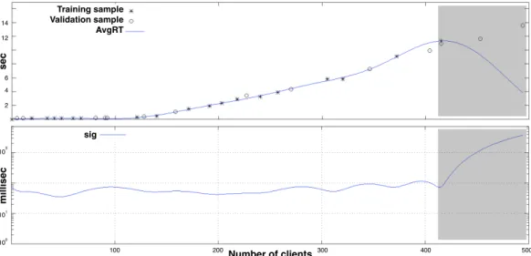
4.1 A Kriging model for predicting performance[31] . . . 57
4.2 Kriging model and confidence interval . . . 58
4.3 Runtime evolution of Kriging models . . . 63
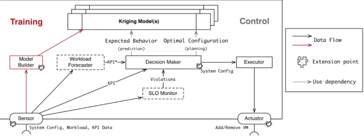
4.4 Conceptual architecture of Kriging-based self-adaptive controllers . . . . 67
5.1 Logical architecture of a Reservoir site . . . 70
5.2 Logical architecture of the Sun grid engine . . . 71
5.3 Logical architecture of the Doodle Web service . . . 71
5.4 Logical architecture of DoReMap . . . 72
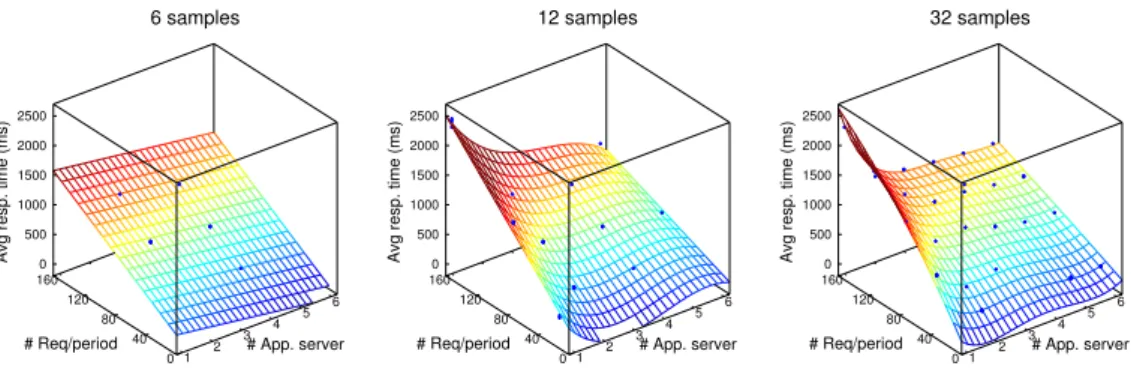
5.5 Different projections of the Kriging model for the Sun grid engine case study . . . 74
5.6 Different projections of the Multidimensional linear regression model for the Sun grid engine case study . . . 74
5.7 Different projections of the Regression tree model for the Sun grid en-gine case study . . . 74
5.8 Different projections of the Multivariate adaptive regression splines for the Sun grid engine case study . . . 77
5.9 Different projections of the Analytical model for the Sun grid engine case study . . . 77
5.10 Different projections of the Combined model for the Sun grid engine
case study . . . 77
5.11 Comparison of models cross validation error . . . 79
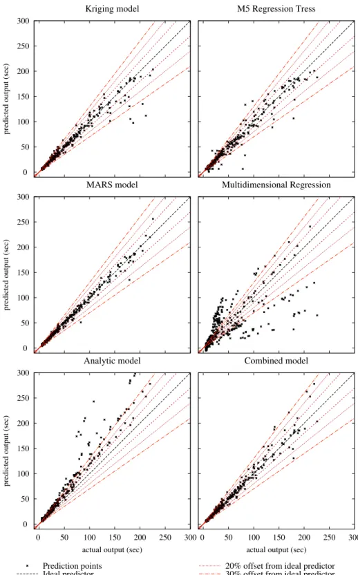
5.12 Actual vs predicted output plots for comparing alternative models . . . . 81
5.13 Dataset 1 for the evaluation of Kriging model robustness. . . 86
5.14 Dataset 2 for the evaluation of Kriging model robustness. . . 87
5.15 Kriging model predictions and prediction error on Dataset 1 . . . 89
5.16 Kriging model predictions and prediction error on Dataset 2 . . . 90
5.17 Data sets for evaluating the improvement of Kriging models over time. . 99
5.18 Adaptation of Kriging models: Heterogenous workload and fast actuators.100 5.19 Adaptation of Kriging models: Periodic workload and fast actuators. . . 102
5.20 Adaptation of Kriging models: Periodic workload and slow actuators. . . 104
5.21 Comparing models improvement . . . 106
5.22 Comparing models improvement . . . 108
5.23 Comparing models improvement . . . 109
5.24 Dataset for evaluating Kriging models adaptation to emerging behaviors 111 5.25 Adaptation of Kriging models . . . 112
5.26 Adaptation of Kriging models . . . 114
5.27 Best models for Experiment 1 . . . 121
5.28 Best models for Experiment 2 . . . 123
5.29 Best models for Experiment 3 . . . 124
A.1 Correlation ofsigand absolute error . . . 136
A.2 Comparison of Kriging and combined models . . . 137
B.1 Combined model predictions and prediction error on Dataset 1 . . . 140
B.2 Regression tree predictions and prediction error on Dataset 1 . . . 141
B.3 MARS predictions and prediction error on Dataset 1 . . . 142
B.4 Combined model predictions and prediction error on Dataset 2 . . . 143
B.5 Regression tree predictions and prediction error on Dataset 2 . . . 144
5.1 Comparison of models prediction ability . . . 78
5.2 Robustness of Kriging models. . . 85
5.3 Robustness of Kriging models: Break down of the first dataset. . . 88
5.4 Comparing model robustness . . . 91
5.5 Promptness of Kriging models for the Sun grid engine case study . . . 94
5.6 Comparison of model promptness for the Sun grid engine case study . . 95
5.7 Performances of controllers in the first experiment . . . 119
5.8 Performance of controllers in the second experiment . . . 120
5.9 Performance of controllers in the third experiment . . . 125
A.1 Comparing Kriging and Combined models . . . 138
B.1 Kriging model accuracy . . . 139
B.2 Kriging models training time . . . 141
Introduction
In this thesis, we explore the use of model-based self-adaptive controllers for dynamic resources allocation: Controllers change the allocation of resources to running systems to avoid violations of service level agreements and to minimize the amount of resources used by the controlled systems. In particular, we propose to use Kriging models as core components for engineering such self-adaptive controllers.
Business organizations and enterprises may provide functionalities to customers by means of Web services, playing in this way the role of service providers. Customers, also referred as final users, are willing to pay for using these Web services but require guarantees on services behavior. For this reason, service providers and final users stipulate contracts, called Service Level Agreements (SLAs) that define what are the expected service behavior and expected service usage. SLAs are commonly expressed in terms of Quality of Service (QoS), i.e., measurable levels of quality attributes, such as availability, reliability, and performance that may be specified over a finite temporal horizon. For example, an SLA may require that a service is always available during working days, that no more than five consecutive service requests fail within two min-utes, or that the service will respond to client requests at least 99.5% of the times in each calendar month with an average response time of five seconds[91]. If the service provider fails to adhere to such contract (i.e., violates the SLA) then clients can claim penalties that result in missed revenues, additional costs, and decreased reputation for the service provider.
Commonly, designers configure enterprise systems so that they can provide the re-quired levels of service. For example, with capacity planning designers decide upon the allocation of resources to systems to provide predictable levels of performances[2]. Capacity planning relies on principles such as resource partitioning and static resources allocation that aim to ensure performance isolation and predictable behavior of ap-plications. It consists of identifying cost-effective system configurations to cope with predefined workload scenarios that are expected to occur at runtime. Designers choose the optimal system configuration according to some high level organization policy. For
example, a company may want to completely avoid SLA violations, while another one may tolerate some amount of violations. In the former case, designers provision the system to cope with the worst scenario that they expect, otherwise, they provision the system to cope only with a fraction of it.
Following these principles, designers tend to provision applications with new re-sources to attain acceptable guarantees on the QoS of services, that is, designers over-provisionthe systems. In this configuration, the costs of ownership for the organization, which include for example costs for cooling, for electric supply, and for maintenance, increase. At the same time, resources are under-utilized for most of the time. As re-ported by several surveys, the average load of servers that are managed according to this model is between 5% and 15%[81; 87].
Besides cost-inefficiency, if design-time assumptions, like the workload distribution, the magnitude of its peaks, or its time-of-the-day dynamics, do not hold, static system configurations may become inefficient, systems may saturate, and services may stop behaving as prescribed by their SLAs. To reduce at the same time the risk of violating SLAs and the average costs of running the enterprise systems, providers can resort to dynamic resource provisioning.
Nowadays, with the advent of virtualization service providers can outsource the management of basic infrastructure resources to Cloud providers, and can cut infras-tructure costs by allocating and deallocating resources to their applications on the fly. More interestingly, service providers can implement dynamic adaptation strategies that automatically react to important changes in the working conditions and modify the system accordingly to avoid violations of SLA. Clouds offer the technical means to dynamically scale applications in order to support a variable number of clients during runtime. They can provision new servers within minutes and remove underutilized servers in seconds.
Problem statement
Unfortunately, Cloud providers do not yet solve the problem of finding the most suit-able configuration that systems should implement to avoid SLA violations. This prob-lem presents some non-trivial challenges: Uncontrolled changes inside the Cloud in-frastructure, unexpected fluctuations and sudden spikes in the service demands, va-riety and complexity of the virtualized applications, and heterogeneity of resources inside the Cloud.
Uncontrolled changes in working conditions of the Cloud may affect the availability of physical resources and the end-to-end QoS of applications that they run. For exam-ple, events like the deployment of new VMs or the failure of some physical machines may have an impact on the virtualized applications. These difficulties depend on the impossibility of directly monitoring these events from the outside of the Cloud.
Clouds are mainly used to run applications that are usually exposed to a large audi-ence and have variable workload. Workload can change in terms of both intensity and
request mix, and this may require different amounts and distribution of resources to application components. For example, the workload may naturally fluctuate consider-ably as its natural request distribution, but it may suddenly increase over a very short time if the service is under a flash-crowd, for example due to a slash-dot effect. These fluctuations may exhaust the available resources and result in service misbehavior and, possibly, in SLA violations.
The kind of systems deployed in Clouds ranges from multi-tier applications, to Web service compositions, content delivery networks, data processing systems, grid middleware and other customized systems[7]. Applications may have complex soft-ware architectures and it is not always clear what are the relationships between system configurations, parameter settings, resource allocations, incoming workload, and the end-to-end application behavior. In the same way, it is not clear what are the effects of acting on any of these concerns at rutime.
Cloud middlewares abstract heterogenous physical resources into virtual machines that from the final user point of view seem to be homogeneous. However, because of this inner heterogeneity different instances of the same virtual machine may show different behavior when run in the same Cloud. This implies that the applications running different virtual machines under a predefined load may provide different end-to-end QoS depending on the actual mapping of virtual machines to physical servers that is not under control of the service provider.
Controllers for dynamic resource provisioning
Service providers resort to controllers that continuously monitor the behavior of con-trolled systems and adapt the configuration of concon-trolled systems to provide a consis-tent level of service.
To be effective, these controllers should fulfill the strong requirements that derive from the non trivial challenges that we identified. For example, controllers should per-ceive unexpected and important changes in the application behavior, and plan actions to reduce the effects of these changes on the application QoS. They should predict ex-pected fluctuations of requests to proactively allocate the right amount of resources, and they should understand if sudden peaks that demand for a quick increase of al-located resources are harming the system. Controllers should also capture the global behavior of applications no matter their internal complexity or number of software tiers. They should learn from the actual perceived situation, update their control strat-egy, and consequently adapt to the working context.
Different solutions are currently available. Controllers that adopt fixed strategies, such as rule-based controllers, may be good if there are no unexpected changes, emer-gent behaviors and the virtual machines behave consistently during the system lifetime. They become less effective when the actual working conditions or system behavior dif-fer too much from design time expectations.
Controllers that are derived from control theory are fast, robust, have tunable pa-rameters and are grounded on a solid mathematical background[66]. They are ap-pealing but difficult to apply because the system identification process at their core is generally too expensive. Furthermore, they require strong assumptions about the linearity of the system behavior to prove properties like system stability and absence of oscillations.
Controllers that exploit machine learning techniques, such as reinforcement learn-ing, are general and do not require any a-priori knowledge. They are proven to pro-duce optimal control policies that are able to deal with unexpected cases and emergent behaviors, but unfortunately they come at the very high costs of exploration.
Model-based controllers exploit models of the system to support their analysis and planning activities. Some controllers use white-box models, like queuing network, while other use black-box and surrogate models.
Controllers based on white-box models are limited by the availability of knowledge about the system internals needed to build accurate models, and by the time required to obtain reliable prediction out of them. In the domain of Clouds for example, there is no visibility inside the system and the parameters of models are difficult to estimate correctly, therefore models can provide only approximate descriptions.
Controllers based on black-box and surrogate models build models of the system behavior by combining input/output data using regression techniques. They are gener-ally applicable because require no knowledge about system internals, and usugener-ally can work with data passively collected from the running systems. Furthermore, black-box models can be adapted or re-trained, thus enabling the implementation of model-based controllers that self-adapt.
In this thesis, we target self-adaptive model-based controllers that exploit black-box and surrogate models to dynamically control the allocation of resources to applications running in Clouds. Despite its application to this specific domain, our solution does not rely on any peculiarity of Clouds, has a general nature, and therefore it can be applied easily in other contexts.
There are a lot of possible models that can be used, but a trade off between accu-racy of representation, costs to manage the model, and time to obtain results out of it is evident: Very accurate models need a lot of data and a lot of time to process them, while simplistic linear models are very fast to train but provide poor predictions. For example, neural networks have the potential to be very effective, but are difficult to setup, have high training costs, and are difficult to interpret once ready. Bayesian trees instead are simpler to build and to interpret but require a lengthy training procedure. Simpler models, like traditional linear regression models, work in less time but at the cost of very rough approximations. Ideally, a model should provide good levels of ac-curacy, with acceptable speed, and at reasonable costs in a way to support controller’s activities without harming its reactiveness.
In this thesis, we propose to use Kriging models as core element of self-adaptive model-based controllers to implement an effective solution that can suitably balance the trade off between accuracy, cost and time of on-line control of complex systems. Kriging models, also called Gaussian process regressors, approximate target functions by means of a spatial correlation between training samples. They extend traditional linear regression with a statistical framework that allows them to predict the value of the target function in un-sampled locations together with a confidence measure.
We choose Kriging models because they are easy to set up, do not require any prior knowledge on system internals, but can accommodate it when available, and because we can use their statistical scaffoldings to implement robust controllers. Compared to other black-box models, they are either more accurate, faster to train and to query, and less expensive to manage.
Kriging-based controllers
We design self-adaptive Kriging-based controllers that exploit Kriging models in differ-ent ways: They analyze monitoring data to iddiffer-entify risky situations that may lead to SLA violations or inefficient use of resources, and they predict the system behavior in different workload scenarios and alternative system configurations. For each service level objective, controllers build a Kriging model that represents the objective metric, for instance the response time or the system throughput, as a function of system con-figuration, for instance the number and types of virtual machines, and a representation of the workload intensity and mix[103].
Kriging models pair predictions with confidence measures, and we leverage this feature to implement robust control policies that weigh the importance of model pre-dictions using their confidence measure, and take informed decisions about the best control strategy to implement. When the confidence of predictions is too low, con-trollers discard them and may resort to alternative strategies or heuristics. For exam-ple, controllers can query other models or take the system to the closest, yet known, system configuration.
Initially, we train Kriging models with data collected by measuring the system be-havior at staging time, and then in production we let controllers continuously update them. By means of model adaptation, controllers adapt themselves to the changing system behavior. As controllers collect more samples, the accuracy of models improve, while their uncertainty decreases, and the time to build the model increases. To avoid the collection of unmanageable sets of samples, many of which do not provide addi-tional information to the model, the controller filters out old samples belonging to the same configuration.
In this thesis, we make the following major contributions:
1) The identification of Kriging models as suitable core components of self-adaptive model-based controllers for dynamic resource management.
2) The design of controllers that exploit Kriging models and implement efficient, ef-fective, and robust model predictive control. The idea behind these controllers is to not only to use Kriging models to predict the immediate system behavior given the actual monitoring data and trigger system re-adaptation, but also to simulate the effects of control actions potentially implementable on the system state while planning the most suitable control strategy.
The proposed approach aims to be general. However, in this thesis, we refer to the domain of applications running in Cloud infrastructure under the Infrastructure as a Service (IaaS) paradigm[109]. We choose this domain because it is significative in the context of software services, is representative of the problem of SLA protection, and encompasses all the complexities that stem from self-adaptive model-based control of complex systems. Cloud IaaS is also increasingly attracting interest from both industry and academia[34; 25; 41].
During the evaluation, we consider only feasible SLAs that pertain to performance and costs. This choice is motivated by the fact that Clouds come with the mirage that systems can scale endlessly, but in practice, either service providers have limited budget or Cloud infrastructures have finite resources. This results in finite size system configu-rations that can sustain only limited workloads under specific SLA conditions. In other words, during the evaluation, we consider only workloads that can be sustained by at least one of the possible resource allocations. In the SLA, we consider performance and costs qualities because they are perceived by service providers and final users as the most important: Costs are primary concerns of commercial companies, in a sense they are also the main driver of the entire Cloud movement. Performance are what greatly impacts on the quality of service as it is experienced by the final users[63].
In the evaluation, we made two more working assumptions. First, we assume that controlled applications can correctly scale without any direct interaction with the controllers. The thesis focuses on the control of elastic applications, but not on their design. In practice, controllers interact with the Cloud platforms to start or stop the virtual machines, therefore we assume that virtual machines are able to automatically join (or leave) the running applications without causing any hard failure. Second, we assume that virtual machines start and stop in near-real time, and consistently across the deployments: It may take up to minutes to have a new instance ready, but there are no strong deviations from this behavior between different deployments. With this assumption, we clarify that controllers can act on the applications as fast as their actuators: If the actuator takes too much time to perform the control actions compared to the application dynamics then the effects of control appear too late, the controller account for long-term predictors, or the SLA is quite tolerant.
1.1
Research Questions
In this thesis, we tackle the problem of design efficient and effective self-adaptive con-trollers that guarantee consistent QoS while efficiently use the resources leased from Cloud infrastructures. We formalize our main research hypothesis as follows:
Research Hypothesis: Kriging models can be used as the core element of
efficient and effective self-adaptive model-based controllers.
In other terms, the thesis proposes the use of Kriging models to build efficient controllers for the Cloud, and investigates the effectiveness of Kriging models in the design and engineering of model-based controllers for the Cloud.
For validating our main research hypothesis, we divide it in two parts: First, we investigate how accurately Kriging models can capture the behavior of elastic appli-cations running in the Cloud. Second, we determine to what extend Kriging models can be used to build efficient and effective autonomic controllers. Following these observations, we refine the main research hypothesis in four research questions.
In the first part, we investigate the accuracy of Kriging models to capture the be-havior of elastic applications in relation to the complexity of elastic applications and the availability of data describing their behavior. We address this issue by means of the first research question:
RQ-1: How accurately do Kriging models capture the behavior of elastic applications
run by Cloud infrastructure?
Proving that Kriging models accurately describe elastic applications is a necessary but not sufficient condition to prove that they can be used inside self-adaptive controllers. In fact, the model accuracy is fundamental for model-based control, as controllers leverage models to predict the potential effects of their control strategies during plan-ning, and inaccurate predictions may lead to ineffective, or even damaging, control strategies. However, beside accuracy controllers require that models have additional properties: They should be easy to set up, to build, and to maintain; they should be robust when data are noisy; and, they should be flexible and adapt to changes of application behavior.
In the second part, we address the issue of the suitability of Kriging models to build autonomic controllers, by investigating the next research questions:
RQ-2: Are Kriging models robust with respect to monitoring data noise and precision? RQ-3: Are Kriging models fast enough to fit the self-adaptive control loop?
RQ-4: Can Kriging models adapt to the behavior of running applications by using the
Research question RQ-2 aims to assure that the accuracy of Kriging models remains sufficiently high to support effective analysis and provide good predictors of applica-tions behavior even when used in real, noisy environments. Research question RQ-3 aims to verify that the predictions are readily available to controllers just when they need them, and that models can be retrained on-line without causing any delay in the control loop. Research question RQ-4 aims to prove that Kriging models have the necessary flexibility to support controllers self-adaptation.
By answering all these research questions, we can prove that Kriging models are indeed suitable core elements to build efficient model-based self-adaptive controllers.
1.2
Scientific Contributions
This thesis advances the state of the art of self-adaptive model-based controllers and controllers for the Cloud by making the following major scientific contributions:
Suitability of Kriging models for control The first contribution is the suitability of
Kriging models in the context of model-based self-adaptive controllers. We show that Kriging models are accurate, robust in real situations, timely in predicting the behavior of applications, and can be trained on-line to implement controllers self-adaptation.
Kriging-based self-adaptive controllers The second contribution is the design of
ef-ficient and effective controllers that we apply in the context of Cloud computing. Our controllers leverage Kriging models to implement robust control policies that account for model inaccuracies by identifying them upfront and by reme-dying with alternative modeling choices. Controllers use Kriging models also to simulate the evolution of system state in the future and provide even more accurate predictions.
1.3
Structure of the Dissertation
The rest of this dissertation is organized as follows:
Chapter 2 presents the background concepts of the work. It describes main concepts
belonging to Cloud computing, Autonomic computing and self-adaptive systems applied in Clouds, and Kriging modeling.
Chapter 3 discusses state-of-the-art solutions that employ controllers for the Cloud,
use surrogate models for performance predictions, and other control solutions that exploits Kriging models.
Chapter 4 describes the solution that we propose in this thesis, i.e., Kriging-based
It motivates the use of self-adaptive model-based controllers, discusses the ra-tionales behind the choice of Kriging models, and presents details on the design and implementation of these controllers.
Chapter 5 describes the evaluation process to validate our solution. The chapter
shows the suitability of Kriging models for modeling applications in the Cloud and the performance of Kriging-based controllers. It critically discusses these results and compares them against related approaches.
Chapter 6 concludes the work. It summarizes our methodology, lists the achieved
scientific contributions, discusses the limitations of our solution, and illustrates the future research that can spring off our work.
Appendices contain additional material and further details about the solution and the
Background
This chapter introduces the basic concepts over which the thesis develops: Cloud com-puting, Autonomic comcom-puting, self-adaptive controllers for the Cloud, and Kriging models.
2.1
Cloud Computing
Clouds provide resources, like computing power, storage space, networking, applica-tions and data as part of large data centers, and offer them on demand as services[8]. Customers access them remotely through the Internet under a pay-as-you-go billing model, and they are charged proportionally to the amount of resources that they con-sume.
From an historical viewpoint, Cloud computing represents the last step of a trend started several years ago with distributed systems, Grids, and Utility computing[7]. This trend moved towards the delivery of services, mainly through the Internet, in a way that resembles the delivery of traditional services by utility companies, such as the one for water and electric power supplies. In this case customers are charged on the amount of resources used and do not participate to infrastructure setup or management.
Taking a different viewpoint, one can see Clouds also as an evolution of traditional Web hosting services. Nowadays, business organizations and enterprises outsource their infrastructures, platforms and applications to Cloud providers to reduce the costs of owning, managing and running IT infrastructures. Furthermore with Clouds, orga-nizations can exploit a set of resources that is unconstrained from their specific com-puting infrastructures.
Clouds are characterized by several aspects: i) The ubiquitous access to resources and electronic services: Everything is on-line and available from everywhere. ii) The opaque management of data and physical resources: Consumers are not able, by design, to locate and directly access the physical systems running their applications.
iii) The on-demand, self-service nature of service provisioning: Consumers can request more or less services, whenever they need, and receive them almost with no waiting time. iv) The usage-based economic model, commonly implemented as pay-as-you-go: Customers pay only for what they actually consume.
Clouds are organized with a strong separation of concerns. Subjects that provide the applications logic, and subjects that are in charge of carrying out the IT manage-ment are agnostic of one other. In this way, service providers can focus on its pri-mary businesses, while Cloud providers takes care of the other duties. For example, if providers want to focus on application development, Clouds can take care of system infrastructure and runtime environments. If providers want to focus on both applica-tions and platform, then Clouds can take care of just resource provisioning. Moreover, Cloud infrastructures allow customers to adjust at runtime their service demand: For example, customers can change the amount of resources allocated to their systems, can deploy new systems and can un-deploy them later on.
Many of distinguishing features offered by Cloud providers are implemented with state-of-the-art technologies and methods that derive from Service Oriented comput-ing[80], Grid computing [12], and system level virtualization [9]. Service Oriented computing has the biggest impact on the management processes relates to the Cloud, while virtualization has the biggest impact resource-wise[58]. As a matter of fact, vir-tualization is the game changing technology that provides isolated execution environ-ments, generally in the form of virtual machines (VM), and the tools for their dynamic allocation, deallocation and management, e.g., checkpoint, replication, cloning, and migration. Final Users Service Providers Cloud Providers LAMP JEE Linux VM infrastructure platform software VM Win Docs Spreadsheet App OS App
Invoke Services Service Service Service
Figure 2.1. Overview of Cloud computing
and delivers basic storage, networking and computational capabilities. The platform is the middle layer. It builds on top of the infrastructure and provides services in an integrated development or runtime environments. Finally, the application is the top layer and offers to final users complete, desktop-like applications as services[64].
Figure 2.1 exemplifies the internal organization of a generic Cloud: Final users access the electronic services as before. Cloud providers manages the “internals” of the Cloud at the different levels. Service providers interact with the Cloud by either managing virtual machines (left), deploying entire applications in predefined environ-ments (center), or composing third party electronic services (right). In these settings, service providers act as final users of Clouds. They buy resources and other services from the Cloud, and use them to provide added value services to their own final users.
Cloud computing defined the three service delivery paradigms:
Software as a Service (SaaS) where clients access complete software systems remotely
and use them as they were on local machines. In this paradigm clients have no control over the application nor the infrastructure. Everything is controlled by Cloud providers.
Platform as a Service (PaaS) where clients provide the application logic and have
the control over its configuration. In this paradigm, Clouds retain the con-trol over the system infrastructure and the middleware components upon which client applications are built. Usually, Clouds provide “sand boxed” environments and clients logic cannot implement critical system level calls.
Infrastructure as a Service (IaaS) where clients provide the whole software that
im-plements the services and Clouds control the system level resources. In this paradigm clients temporarily acquire remote and isolated virtual servers over which they have full control.
This thesis develops its contributions in the context of Cloud IaaS. We target plat-forms that offer infrastructure level resources as services, and run virtual machines on behalf of service providers. Service providers control the lifecycle of virtual ma-chines, while Clouds implement management actions like virtual machines placement and physical resources allocation. In essence, IaaS enables service providers to add or remove virtual servers on the fly, and dynamically scale their systems. Service provides use this feature to implement elastic applications that can be adapted to dynamically changing working conditions.
Commercial IaaS platforms, like Amazon Ec21, RightScale2, Scalr3, and many oth-ers, come with basic tools to automate the scaling of customer applications. These tools share the same threshold-based basic pattern: Service providers select a subset of the
1http://aws.amazon.com/ec2/
2http://www.rightscale.com/
application variables monitored by the Cloud platform, specify a set of conditions over their values, and specify how to react when those conditions are met. For example, service provider can monitor the average CPU usage of virtual machines, set a thresh-old on its value, add a new virtual machine whenever the average CPU usage passes the threshold. In this systems, Cloud providers take care of monitoring the system variables, checking all the conditions, and triggering the specified control actions.
Service providers manually specify these rules and have no tools other than their personal experience to check the suitability of their choice. Also commercial platforms have no tools to support the discovery, update and management of the rules: If the system behave differently from the service providers expectations service providers have to disable, modify and re-enable all the rules.
Static threshold- and rule- based strategies are intuitive and easy to understand, and they may be the right choice for cases when service providers can make strong assumptions on their systems or applications have simple software architectures. How-ever, as the situation becomes more complex, for example, in case of highly dynamic workload, more complex software architectures and unexpected events, fixed control strategies may not be cost-effective.
These situations require solutions that react to known, predictable and recurrent events, that predict the behavior of complex applications, and that proactively react to unexpected or potential risky situations. An ideal solution should be able to learn from its past experience and update its control strategy in spite of that, possibly with little or non human intervention, as fostered by the autonomic computing community.
2.2
Autonomic computing and self-adaptive controllers
Autonomic computing is about the idea of systems that can automatically and au-tonomously manage themselves according to high level objectives defined by system administrators[38].
The central element in the implementation of autonomic computing is the auto-nomic element, also called autonomic controller. Autonomic elements work in a closed loop with the systems they control: They sense the environment and the main vari-ables of the controlled system, and then apply control actions to modify it. In between sensing and acting, controllers implement activities that logically form a loop4, usually called the MAPE-K loop[40]. In the MAPE-K loop, controllers monitor data (M), an-alyze (A) them to plan (P) a suitable control strategy, and execute (E) the strategy by implementing the control actions on the system. In all of these activities, autonomic controllers rely on some knowledge (K) about the controlled systems and environ-ment[53].
4The activities of autonomic controllers are not necessary executed in sequence, even if this is the most common pattern.
This thesis focuses mainly on the two central activities of the loop, i.e., analysis and planning, and the knowledge component.
Se n so rs Act u a to rs Knowledge Monitor Execute Analyze Plan
Figure 2.2. Autonomic element
The high level objectives that controllers try to achieve may concern several as-pects, called self-* properties, that include: optimization, configuration, fault tolerance and security. Self-optimizing systems aim to maximize some utility function of the system; self-configuring systems adapt the software architecture to dynamic environ-ments; self-healing systems recover from failures; and, self-protecting systems deal with security attacks.
Simple self-* systems usually deal with only one property, while more advanced solutions deal with many properties at the same time. This thesis is centered around the design of controllers that provide the system mainly with optimizing and self-configuring abilities.
Common controllers architectures
Controllers come in different flavors and with several architectures as discussed by Brun et al.[15] and Patikirokorala et al. [83]. Authors group controllers in centralized and distributed depending on their architectures.
Centralized controllers are the most common solutions and refer to centralized single-controllers and centralized multi-controllers.
Figure 2.3 exemplifies some centralized controllers as block diagrams: I) Feedback controllers. They use output of the system to compute an error metric and plan a con-trol strategy that reduces it. II) Feed forward concon-trollers. They receive the same input signals of the controlled system and compute the control strategy on them. III) Feed-back and feedforward controllers. They combine the former two controllers in a single solution. IV) Model predictive controllers. They employ a model of the system in con-junction with an optimization procedure to define the control strategy: At each control interval, controllers simulate the system using the model and plan the best strategy over a receding horizon. V) Cascading controllers. They chain two multiple controllers such that outer controller controls the inner controller, and the inner controllers act on the system. VI) Multi controllers with switching. They run several controllers in parallel and use them in mutual exclusion to control the system.
Distributed controllers are the alternative to centralized controllers and their con-trol logic is deployed over multiple concon-trollers. We report the most common
archi-Target System A S Controller Set point Control error Control input System output Feedback controller Target System A S System output Controller Control input Disturbance
Feed forward controller
Target System A S Feedback controller Set point Control error Control input System output Feed forward controller Disturbance
Feedback, Feed forward controller
Model Optimization Set point Target System A S Control input System output
Model predictive controller
Cascading controller Outer controller Set point Inner controller Target System A S Control input Set point System output Target System A S System output Controller 1 Controller 2 Controller n Control input Control switch
Multiple controllers with switching
Figure 2.3. Block diagrams of centralized controller architectures [83]
tectures of distributed controllers in Figure 2.4: I) Hierarchical controllers. They are organized hierarchically, and controllers in upper-level act on controllers in the lower-levels, and eventually on the target system. II) Fully distributed controllers. They are composed of independent local controllers that communicate over a shared communi-cation substrate. Controllers collaborate to fulfill the control goals.
Hierarchical controller Target System Subsystem 1 Subsystem 2 Subsystem n Level 0 Controller Level 0 Controller Level 0 Controller Level 1 Controller Level 1 Controller Level 2 Controller
Fully distributed controller Communication Target System Subsystem 1 Subsystem 2 Subsystem n Controller 1 Controller 2 Controller n
Figure 2.4. Block diagrams of distributed controller architectures [83]
Controllers presented so far assume that the system behavior is stable and that all the system identification activities are done before going live. This is not always possible because the controlled systems and the environment may show transient and emerging behaviors, or because an extensive model identification is too expensive.
Self-adaptive controllers instead are able to adapt as the system behavior changes. Controllers adaptivity is a concept taken from advanced control theory where it is usually implemented in the form of automatic tuning of controller parameters or track-ing of hidden variables[116]. In the context of autonomic computing, self-adaptivity has a broader meaning than parameter estimation and variable tracking, and encom-passes also updates on control strategies and structural changes of controllers internal architecture[15].
In Figure 2.5, we illustrate the block diagrams of generic adaptive and self-tuning controllers. Self-self-tuning controllers employ an estimator component that tracks the hidden variables and provides the controller with their values. Self-adaptive con-trollers employ a reconfiguration layer that acts on the control layer to adapt it. For example, Magee and Kramer propose a three-layered control approach where an high level goal management layer controls the underlying levels for change management and software components[53].
Self-tuning controller Three-later self-adaptive controller
Target System A S controller Set point Control error Control
input Systemoutput Estimator Parameters Target System A S controller Specification Goal management Change management
Figure 2.5. Block diagrams of common self-adaptive controllers
In this thesis we focus on centralized controllers, in particular on model based self-adaptive centralized controllers, to tackle the problem of dynamically control elastic applications in the Cloud: The control strategy is derived from models that describe the system behaviors that are adapted at runtime. We choose the centralized approach over the distribute one, because it is conceptually simpler and easier to manage, and we choose a model based controller because is more flexible and generally applicable than standard feedback and feedforward solutions.
2.3
Autonomic and self-adaptive controllers for the Cloud
Autonomic and self-adaptive controllers are designed to deal with complex systems, highly dynamic environments, uncertainty and emerging behaviors. Additionally, they can learn from past experience[49]. These characteristics make them a sensible choice for managing elastic applications running in Clouds. In fact, Clouds are very dynamic environments that provide high degree of automation to carry out all the management tasks, and host complex applications that may be composed of several interdependent
software components, and may face highly variable workloads.
In Cloud settings, state-of-the-art approaches that are based on autonomic com-puting principles can be classified as: (i) approaches used inside the Cloud to perform activities on its internals, such as controlling resources allocation between the hard-ware and virtualized layers, (ii) approaches used outside the Cloud to perform activ-ities that target user applications and leverage Cloud features , and (iii) approaches that combine the previous two.
Inside the Cloud, controllers are applied mainly for optimization goals: For ex-ample, they are used to optimize the placement of virtual machine to minimize the number of active physical servers (server consolidation)[16]. Or they are used to ad-just the CPU frequency of physical servers to improve their power efficiency while maintain VM-related metrics to specified levels[48; 92].
Outside the Cloud, controllers are commonly used to manage final users applica-tions: For example, they are used to control the horizontal and vertical scale of elastic applications, or to dynamically migrate VMs between physical machine, data centers, or federated Clouds to maintain acceptable levels of dependability.
The focus of the thesis is on the use of autonomic approaches outside the Cloud, that is, exogenous controllers[115]. We make this decision bearing in mind generality and separation of concerns: By developing controllers that run outside the Clouds we can reuse the same controller across different Cloud infrastructures as long as the controlled application remains the same. Furthermore, by running controllers on the side of service providers, we leave full control to service providers on the controllers if they want to remove, change, or update them. This is different for example from the approach offered by Amazon and other Cloud providers that allow service providers to specify rules, but fully control their execution.
We design controllers that operate on behalf of service providers and manage their elastic applications at runtime: Controllers bind public interfaces exposed by Clouds, monitor applications behavior and billing status, and take informed decisions that trade off running costs and quality of service before acting upon the virtualized in-frastructure. In particular, controllers take decisions about what type and how many instances of virtual machines have to be replicated or removed, and when to implement the control actions.
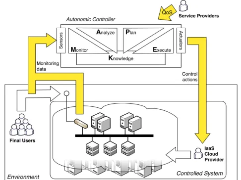
In this thesis, we follow the reference architecture for self-adaptive controllers and we adapt it to fit the Cloud domain. Figure 2.6 shows the resulting situation: The controlled system is a virtualized application that runs inside the Cloud. The Cloud is operated by an IaaS Cloud provider. The environment embeds both the controlled system and the Cloud. Final user perturb the application by means of the service invocations. The controller lies outside the Cloud, monitors the invocations by the final users and the service behavior, and invokes operations at the infrastructure level on the Cloud.
Environment Final Users Controlled System IaaS Cloud Provider Se n so rs Act u a to rs Knowledge Monitor Execute Analyze Plan
Autonomic Controller Service Providers
Control actions Monitoring
data
QoS
Figure 2.6. Reference architecture for autonomic controllers in the context of elastic applications and Cloud IaaS
2.4
Kriging models
This thesis proposes Kriging models as the basis to build self-adaptive model based controllers. This section introduces Kriging modeling, focusing on the aspects of in-terest in this thesis. The inin-terested reader can find a comprehensive presentation of Kriging models in[90; 107].
Kriging models were defined in the context of mathematical geology by the French mathematician Georges Matheron [72]. They are named after Daniel G. Krige, the South-African mining engineer who firstly proposed them in the 1950s [54]. Origi-nally, Kriging models were proposed to approximate the underground concentration of valuable minerals by interpolating samples taken at different locations, and gradually they have been used in other contexts. Starting from the seventies, Kriging models have been used to develop approximations5 of deterministic and expensive simulation for designing optimization functions in domains such as geo-statistics, meteorology, avionics and circuit design[94]. Recently, Kriging models have been used in Machine Learning, where they are known as Gaussian processes[90].
Kriging models are a family of black box models that approximate non linear multi-modal functions. They are build starting from a training data set and capture the rela-5In relation of this application as approximations of simulations Kriging models are also referred to as
x1 x2 Input, x O ut put , y x1 x2 Input, x x1 x2 Input, x Figure 2.7. Example of regression with Gaussian Processes [88]
tions among input and output data, a process commonly known as supervised learning. Once trained, they predict output values at input locations that were not present in the training set and that we denote by x∗. Kriging models are suitable for regression problems when inputs and outputs refer to continuous dimensions, but can also be used for classification problems that involve non-continuous features[23]. Figure 2.7 shows how Kriging models works over a simple example taken from [88]: The left panel reports the training points (as black dots) that we use to train a Kriging model to predict the output function ( y). The panel highlights two unknown points (x1and x2) that we want to predict with the model. The central panel shows the Kriging model that results from the training data (as solid gray line). For x1and x2, the panel shows also the confidence interval that is associate with the predictions as error bars centered in x1 and x2. The right panel shows the complete Kriging model. In this panel, we plot the model predictions and the corresponding confidence area for the whole input space.
Kriging models have many interesting properties: (i) They are global, i.e., they span over the whole input space, differently form classic regression models that are commonly preferred for local predictions. (ii) Whenever it is assumed that data are noise free, like in the context of deterministic computer simulations, Kriging models produce the exact interpolation of data. Otherwise, they implement a form of data smoothing. (iii) Kriging models can provide a measure of the uncertainty of their own predictions; this measure accounts for both the availability of training samples, their distribution over the input space, and their level of noise. (iv) Kriging models in general do not need a very large amount of training samples to provide acceptable predictions, thus are relatively fast to train.
Kriging are a valuable alternative to other black-box models, either classic regres-sion methods that are based on first- or second-order polynomials, and non-parametric models, such as smoothing splines and radial basis functions[107]. Differently from classic models like artificial neural networks (ANNs) or traditional linear regressors
that require extensive configurations in terms of layers, neurons and model degrees to match systems complexity, Kriging models are easier to use because they automatically search for the relationships among measured data in the scope of a fixed, but very expressive, internal structure.
Both ANNs and Kriging models can be used as black-box models to predict not yet experienced values, but only Kriging models can be inspected and interpreted to better understand the properties of the predicted values: By inspecting the model after the training, we can derive conclusions about the relative influence of each input dimension on the modeled output, and this can be used, for example, to filter out not-informative input features, thus reducing the complexity of the model itself[90].
As any other approach based on data, Kriging models depend on the availability and the quality of training data to make accurate prediction. However, Kriging mod-els can leverage an uncertainty measure to identify regions in the input space where training data are scarce compared to the complexity of the unknown function. We can use this measure to account for the reliability and risks of using the values predicted by the models.
The remaining sections give an intuition on how Kriging models work along with the two main point of view: Kriging models as extensions of traditional linear regres-sion, and Kriging models according to the Bayesian theory.
Internals of Kriging models
Given a training set consisting of input vectors (xi) and corresponding observations ( yi), the aim of supervised learning is to infer a model of the (unknown) function ( f )
that has generated the data. The model of the unknown function is generally given by a linear combination of parameters and functions to be estimated.
ˆy = f (x) + ε (2.1)
whereε is the error term. Observations are assumed independent and identically dis-tributed (i.i.d) and the error is assumed Gaussian with zero mean and given standard deviationσ2ε.
Two main viewpoints describe how Kriging models work: According to the first, Kriging models extend traditional interpolation methods with a statistical framework based on stochastic processes6, typically Gaussian processes [23]. According to the second viewpoint, Kriging models can be framed in the Bayesian theory in terms of prior and posterior distributions, likelihoods and observations.
6Stochastic processes generalize stochastic distributions to functions: A distribution describes a ran-dom variable, while a process describes a ranran-dom function.
Kriging model as extensions of linear regression
As summarized by Jones et al. [45], Kriging modeling can be interpreted as an ex-tension of classic regression with stochastic processes. In fact, they share a common mathematical framework that includes regressors and errors, but they put different emphasis on the two aspects: Classic regression focuses on the regressors and their co-efficients, and makes simplistic assumptions about the errors and their independence. Kriging modeling instead focuses on the correlation structure of the errors, and makes simplistic assumptions about the regressors. In other words, classic regression is about estimating regression coefficients that together with the assumed functional form fully describe what the function is about, while Kriging modeling is about estimating corre-lation parameters that describe how the function typically behaves, thus describing how much the function tends to change while moving along different input dimensions.
Kriging models correlate training samples by assuming that the target function is continuous and that there is a spatial correlation between observations: Samples that are close to each other in the input space have similar output values. Kriging models capture this correlation by exploiting the error terms: ε is modeled as a stochastic process and it depends on the observation, therefore it can be re-written as ε(xi). From the assumption of continuity of the unknown function and the general trend, it follows thatε(x), which is computed as their difference, must be continuous too. And for any two points close together (xiand xj) the corresponding errors terms (ε(xi) and ε(xj)) should be also close.
Figure 2.8 captures this intuition over a simplified example that we take from[45]: The thick line represents the unknown function, and the black dots represent the col-lected observations. Let’s assume that there is no additive noise in the data and that the empirical mean (ˆµ) is the global trend, which is represented as a thin line in the diagram. According to the theory, given an xi, the error termε(xi) is computed as the distance between the model, which is ˆµ, and the actual value of the function yi. From the figure, we can intuitively see that error termsε(x∗) and ε(xi) that corresponds to the unknown location x∗and the nearby location xi have similar values.
Unknown function Global trend Unknown function
Global trend
Figure 2.8. Error correlation in Kriging models [45]
Kriging models capture the correlation of samples in a correlation matrix that we denote by K. Given K, Kriging models predict the value of the target function in the unknown coordinates x∗ as the most consistent value with respect to the estimated
typical behavior of the function that is summarized by best linear unbiased predictor: ˆy(x∗) = µ(x∗) + kT K−1 (y − µ(x∗)1) (2.2)
The first term of the predictor is the evaluation of the mean at the untrained input and the second term is the adjustment that is based on the correlation among the errors. It must be noted that, if there is no correlation (k= 0) the predictor reduces to the mean (ˆµ), while at a sampled points (k=Ki) the predictor interpolate the data. In between these extremes, ˆy is based on a smooth interpolation of the data
The estimation of accuracy of the prediction is affected by the correlation of the error terms and it can be measured as the mean squared error (MSE) with the following formula:
s2(x∗) = σ2ε[1 − kTK−1k + (1 − 1
TK−1k)2
1TK−11 ] (2.3)
The term kTK−1k represents the reduction in prediction error due to the fact that x∗
is correlated with the training points, i.e., no correlation implies no adjustment. The term(1 − 1TK−1k)2/1TK−11 reflects the uncertainty that stems from not knowing the
function exactly.
Kriging model according to the Bayesian view
Kriging models can be interpreted also according to the Bayesian theory. This is the viewpoint of the Machine Learning community, and is summarized by Rasmussen et al.[90].
The inference process starts with a prior distribution over a set of possible func-tions that may represent the unknown function. In this particular case, the prior is a Gaussian process and samples drawn from the unknown function are assumed to be normally distributed. Their covariance is assumed to be depend on samples spatial location, i.e., the distance between them. The prior is combined with a set of observa-tions, i.e., the training points, to obtain the posterior distribution that is used to make the predictions. This combination is governed by the Bayes rule:
posterior= likelihood× prior marginal likelihood
The prior encapsulates all the knowledge that is available at the beginning, i.e. before collecting any data. In our context, the prior encapsulates the expectations over the kind of functions to be observed: Smooth functions with stationary variance. The in-formation from the training set are used to derive the likelihood and the marginal like-lihood (or evidence). Finally, the resulting posterior, which is also a Gaussian process, describes the expected behavior of the function as was derived from the observations. Figure 2.9 gives the intuition of the inference process with the Bayesian model in a simple example. We take the example from [90]. The left panel shows some of
the distributions (as solid lines) that are drawn from the Gaussian process used as prior. The same panel highlights also the confidence interval of the Gaussian process as gray area. The right panel instead shows how this evolves after the observation of two samples. The panel shows some distributions (as dotted lines) that are drawn from the resulting posterior and the confidence interval. In particular, and as the intuition suggests, the confidence interval adapts to the data: It is reduced close to the observations while is not changed away form them.
Figure 2.9. Bayesian inference with Gaussian processes [90].
Informally, the net result of this inference process is that some of the potential dis-tributions that could be drawn from the prior are filtered out with the observations: Distributions that behave according to the original prior and the data are retained while the others, which do not interpolate the observations, are removed. Once the posterior is available, its mean function computes the predictions and its variance (at the prediction locations) computes their uncertainty. The figure shows the mean func-tion of the posterior as solid bold line.
This theory involves the computation of several integrals and other complex math-ematical operations, but by focusing on stochastic processes that are Gaussian, it turns out that these computations become relatively easy as the model can be treated ana-lytically. We can write the general model (see 2.1) in terms of the parameters w and make inference on them7:
f(x) = xTw (2.4)
In this formulation, the problem is to find the value for the parameters using the Bayes rule, i.e., find the posterior distribution of the parameters given the prior and the observations
p(w|X, y) = p(y|X, w)p(w)
p(y|X) (2.5)
In absence of evidence, the common prior (p(w)) is the zero mean Gaussian with covariance matrixΣp. This choice is not a huge limitation because the resulting poste-rior will have a mean that is different from zero because that depends on the training data. Of course, whenever some a-priori knowledge is available, it can be plugged in the model by defining a suitable prior.
Thanks to the independence assumption of the observations, we can factor the likelihood over the training points to obtain
p(y|X, w) = n
Y
i=1
p(yi|xi, w) = . . . = N (XTw,σ2εI) (2.6)
which is Gaussian. Finally, the marginal likelihood is independent of the parameters and is given by
p(y|X) = Z
p(y|X, w)p(w)dw (2.7)
It can be shown that the posterior is Gaussian and is given by
p(w|X, y) ∼ N (w, A−1), where (2.8)
A = σε−2XXT + Σ−1p , and
w = σε−2A−1Xy
The model computes the prediction for a given input by averaging over all the possible parameter values weighted by their posterior probability. The prediction and its uncertainty are given again by the mean and variance of a Gaussian distribution that correlates test input with the observed values in a well defined form.
p(y∗|x∗, X, y) = Z p(y∗|x∗, w)p(w|X, y)dw = ... = N ( 1 σ2 ε x∗TA−1Xy, x∗TA−1x∗) (2.9)
Sample correlation is the central point of Kriging modeling
In their more general formulation, Kriging models contains two terms: The first is called global trend and is meant to capture model-wise variations; the second instead accounts for local modifications and it is implemented by means of Gaussian processes. Universal Kriging models put no constraints on the global trend, Ordinary Kriging models assume a constant but unknown global trend, while Simple Kriging models as-sume a known constant trend that, by convention, is equal to zero. These models allow for different levels of expressivity, but in any case, the most important part remains the correlation function.

![Figure 2.9. Bayesian inference with Gaussian processes [90].](https://thumb-eu.123doks.com/thumbv2/123doknet/15027993.686503/38.892.158.728.329.573/figure-bayesian-inference-with-gaussian-processes.webp)