Evaluating the effect of climate change on groundwater resources : from local to catchment scale

(1)

Evaluating the effect of climate change on

groundwater resources:

From local to catchment scale

Thèse présentée à la Faculté Science

Centre d’hydrogéologie et géothermie (CHYN)

Université de Neuchâtel

Pour l’obtention du grade de docteur ès Science

Par

Christian Möck

Acceptée sur proposition du jury :

Prof. Daniel Hunkeler, University of Neuchâtel, Switzerland, directeur de thèse Prof. Philip Brunner, University of Neuchâtel, Switzerland, co- directeur de thèse

Prof. Alain Dassargues, University of Liège, Belgium, rapporteur Prof. Richard Taylor, University College London, England, rapporteur

Soutenue le 11.11.2013 Université de Neuchâtel

(2)

(3)

2000 Neuchâtel - Suisse Tél: + 41 (0)32 718 2100 E-mail: [email protected]

IMPRIMATUR POUR THESE DE DOCTORAT

La Faculté des sciences de l'Université de Neuchâtel

autorise l'impression de la présente thèse soutenue par

Monsieur Christian MOECK

Titre:

Evaluating the effect of climate change on groundwater resources :

From local to catchment scale

sur le rapport des membres du jury composé comme suit:

x Prof. Daniel Hunkeler, Université de Neuchâtel, directeur de thèse x Prof. Philip Brunner, Université de Neuchâtel, co-directeur de thèse x Prof. Alain Dassargues, Université de Liège, Belgique

x Prof. Richard Taylor, University College London, UK

Neuchâtel, le 20 mars 2014 Le Doyen, Prof. P. Kropf

(4)

(5)

Mots clés en français : Changement climatique, renouvellement de la nappe

phréatique, simplification de modèle, fréquence des sécheresses, effets des plantes Mots clés en anglais : Climate change, groundwater recharge, model simplification, crop effect, drought frequency

(6)

(7)

1

Abstract

There is strong evidence that climate is changing and will affect the water resources. A major question arising from the evaluation of climate change (CC) impacts on groundwater resources is to what extent groundwater recharge will change. Given that for Switzerland, climate models predict more frequent hot and dry summers in the future while precipitation will tend to increase in winter, a special attention was given to possible changes in the seasonal distribution of recharge. However, to provide robust predictions, uncertainty has to be considered in all simulations. Three uncertainty sources can be distinguished: the latter can originate from climate models uncertainty, the unknown evolution of land use and society in general, and the hydrological models themselves. The role of these three types of uncertainty has received a major attention in this study. Three studies were carried out to evaluate the effect of CC on the hydrological system. Two of these studies were dedicated to the topic of groundwater recharge whereas the third was focused on the CC response of an aquifer system.

The first recharge related study deals with the question of how uncertainty due to climate models interacts with uncertainty associated with different hydrological models. Although different models were used to simulate groundwater recharge in numerous climate impact studies, it is not yet clear whether models of different complexity give similar recharge predictions for a given climate scenario. Therefore, five different commonly used approaches to simulate groundwater recharge were compared under CC.

In this analysis models with different complexity were applied over a time span of several years and predictive model bias occurs. Using CC data with more extreme weather conditions increases the resulting bias. The potential for model predictive error increases with the difference between the climatic forcing function used in the CC predictions and the climatic forcing function used in calibration period. The difference between the reference recharge and simulated recharge from physical based but homogenous model as well as semi-mechanistic model are smallest whereas the differences increase with the simple models. The differences are due to structural model deficits such as the limitation of reproducing preferential flow. Thus, results of CC impact studies using the soil water balance approach to estimate recharge need to be interpreted with caution, although the majority of CC impact assessment studies are using this approach. Comparison of both uncertainties, i.e. CC and model simplification, indicate that the highest uncertainty is related to CC, but a model simplification can also introduce a significant predictive error.

The second recharge related study explores how different crops and crop rotations influence CC effects on groundwater recharge. The predicted temperature increase will doubtlessly lead to an increase in evaporation and can be intensified by the

(8)

2

presence of crops. To address this question, we relied on lysimeter data to ensure that the models represent previously measured crop specific effects on groundwater recharge appropriately before attempting to simulate future trends. In addition to effects of crop types, effects of soils types were considered. To study the effect of soil types on recharge was possible thanks to the presence of three Swiss dominant soil types in the lysimeter facility. This study attempts to explore the combined effect of CC and changes in land use on groundwater recharge. We address these questions by combining numerical modeling techniques with high quality lysimeter data. The simulated results of the 1D numerical model indicate that for most crops a decreasing trend occurs (between -5 to -60%) due to higher evapotranspiration rates. However, for catch crops (fast-growing crop that is grown between successive plantings of a main crop) such as Phacelia and Temporary grassland, an increasing recharge trend can also be observed (up to 15%). Using these catch crops in a crop sequence can buffer the decreasing trend in future recharge rates, but the buffer capacity depends strongly on the growing season.

It is very likely that crop parameters such as leaf area index (LAI) and root depth (RD) will change in future due to increasing water stress (reduced water content in the lysimeter). Therefore, an analysis of the sensitivity of LAI and RD on recharge was carried out. It was found that simulated recharge is inversely related to LAI and RD where recharge is more sensitive to a decrease in LAI than to RD. Therefore, recharge estimates based on literature LAI and RD values probably represent an upper boundary on recharge rate changes for the future. However, in all simulations a high predictive uncertainty in results is given due to the variability originating from general circulation model (GCM) and regional climate model (RCM) combinations and stochastic realisations of the future climatic conditions.

The final study explored how changes in groundwater recharge might influence groundwater levels for a small aquifer used for water supply. The soil-unsaturated zone-groundwater system was considered as a whole using the physically based model HydroGeoSphere (HGS). The model was based on a wide range of field data. The main objective of this part was to evaluate if seasonal shifts of groundwater recharge can lead to lower groundwater levels in late summer and a potential water shortage. Such effects are mainly expected for highly transmissive systems with a low storage capacity that are expected to react rapidly to seasonal variations in recharge. Therefore, a small aquifer consisting of highly permeable glacio-fluvial deposits and used for water supply for a small town was selected.

The physically based model HydroGeoSphere (HGS) was used to simulate changes in recharge rates and groundwater levels based on 10 GCM (Global Circulation Model) - RCM (Regional Climate Model) combinations for the A1B emission scenario. Future recharge rates were compared to rates observed during historical drought periods. The recharge drought frequency was quantified using a threshold approach. The flow simulations indicate that the strongest effect of CC on recharge occurs in autumn and not in summer, when the temperature changes are the highest. For the winter season, recharge rates increase for almost all climate model chains and

(9)

3

periods. In summer and autumn, temporal water stress, which is defined as reduced drinking water supply, can occur but the intensity depends on the chosen climate model chain. The uncertainty which comes from the variability among different model chains is large although all climate model chains show the same trend in the recharge seasonality. An estimation of drought frequency for a “worst-case” scenario indicates an increase in frequency and intensity under predicted CC. For the water supply in Wohlenschwil, water shortage will most likely more frequently occur in summer and autumn whereas no water stress is predicted for all other seasons.

All studies demonstrated that the uncertainty surrounding projected recharge rates and groundwater levels are relatively large. Some model chains indicate decreasing recharge and groundwater levels until the end of century, while other show increasing trends. For instance for the Wohlenschwil aquifer a change in annual recharge between -16% and 12% was simulated, while the mean of all climate model chains indicate no changes. Therefore, it is quite difficult to state on the magnitude of the change with high confidence. However, not the mean is important, but rather the seasonality. Almost all climate model chains lead to a change in seasonality but with a different magnitude. In addition, the uncertainty linked to the interannual variability of the climate is highly uncertain and can lead to strongly different results and conclusions depending on analyzed equiprobable stochastic realisations. However, the main uncertainty is linked to GCM-RCM combinations. This uncertainty is followed by the uncertainty originated by natural variability of the climate and model simplification. The calibration of the hydrological model is a further uncertainty, but could be reduced by improving the model calibration, if needed.

Although uncertainty in all predictions makes it difficult to state on the magnitude of the change with high confidence, it becomes obviously that a proper consideration of possible effects of CC on groundwater are needed. Results indicate that groundwater is only slightly effected in northern Switzerland on an annual basis but temporal changes can lead to periods with low recharge rates and groundwater tables and therefore to limit water supply.

(10)

(11)

5

Acknowledgments

I have been very happy and proud to perform this research at the Centre of Hydrogeology and Geothermics (CHYN), a very inspiring research environment with great colleagues. Of course, there were a lot of people supporting me during my study and I would like to thank all them gratefully.

A special thanks to Daniel Hunkeler and Philip Brunner who supervised this thesis. I would like to thank for support, mentoring and openness to discussion. Thanks for raising new ideas after each discussion.

Thank you to Richard Taylor and Alain Dassargues who have accepted to join the jury of this thesis and to take time to read this report.

I wish to thank Volker Prasuhn for his guidance and patience, while introducing me into the world of lysimeters. I also would like to thank Mario Schirmer for taken always time for meetings about the project and providing support of various issues. I wish to thank John Doherty for his support in using his code PEST. His support at the initial state of my study prevent a lot of frustrations and headache about PEST. Special thanks to Daniel Käser, we shared the office for 3 years, Oliver Schilling and Daniel Partington for discussions about hydrological modeling and private issues. You guys were being such a pleasant office mates.

The fieldwork would not have been possible without the guidance of Roberto Costa. Thanks for helping me in the field and solving all technical problems. I would like to thank also Antoine Baillieux, who was working with me at the Wohlenschwil catchment. I really enjoyed the fieldwork and discussion with you. I want to thank my colleagues at the CHYN for a good balance between work and pleasure, making my PhD years to such a pleasurable experience. A special thanks to Alice, Philip, Jessica, Yuexia, Oliver, Daniel K., Daniel P., Daniel B., Jordi, Simon, Florian, Bibiane, and Fabio.

Thanks to Swiss National Foundation NFP61 “Sustainable water resources”, which allowed me to carried out this research.

I am very grateful to my friends for their support and for making life outside the office so appreciated. Last but not least I wish to thank my family. I am very grateful to my family for their love and support. Thanks for everything. Particular thank to Katrina and my daughter Nele. Your daily smiles makes every day so worthwhile. Neuchâtel, October 2013

(12)

(13)

7

Table of Figures

Figure 2. 1: The three pathways of anthropogenic greenhouse gas emissions, along with projected annual mean warming for Switzerland for the 30-year average centered at 2085 (aggregated from the four seasons and three representative regions). These pathways are based on assumptions about global demographics and societal development, energy demand, technologic and economic trends, and corresponding decisions and choices that our world is taking now and may take in the future. The unit «CO2eq» is a reference unit by which other greenhouse gases (e.g. CH4) can be expressed in units of CO2. (Figure taken from CH2011

(2011)). 24

Figure 2. 2: Schematic illustration of the utilized model chains of the ENSEMBLE project, all using the A1B emission scenario. Short and long RCM-bars represent simulations that cover the periods 1951–2050 and 1951–2100, respectively. All model chains marked by stars (***) have been used in this PhD. (Figure taken

from CH2011 (2011)). 26

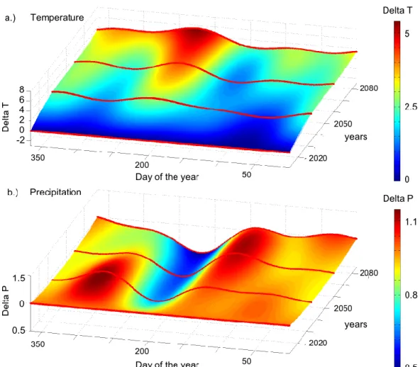
Figure 2. 3: Linear delta change factor interpolation between the year 2011 and the three time periods 2035, 2060 and 2085 (red lines) for a.) temperature and b.) precipitation for each year from 2011 to 2085 and each day is shown. Red and blue colors indicate increase and decrease trends, respectively. 28 Figure 2. 4: Past and future changes in seasonal temperature (°C) and precipitation

(%) over northern Switzerland. The changes are relative to the reference period 1980–2009. The thin colored bars display the year-to-year differences with respect to the average of observations over the reference period; the heavy black lines are the corresponding smoothed 30-year averages. The grey shading indicates the range of year-to-year differences as projected by climate models for the A1B scenario (5–95 percentile range for the available model set). The thick colored bars show best estimates of the future projections, and the associated uncertainty ranges, for selected 30-year time-periods and for three greenhouse gas emission scenarios. (Figure taken from CH2011 (2011)). 30 Figure 2. 5: Illustration of potential changes in frequency and intensity of temperature

and precipitation extremes in a changing climate. Current and potential future distributions are depicted with full and dashed lines, respectively. Changes in the distribution of temperature and precipitation (mean, variability and shape) potentially lead to changes in the frequency and intensity of hot, cold, wet and

dry extremes. (Figure modified from CCSP 2008). 31

Figure 2. 6: Cascade of uncertainty for CC impact studies in hydrology. Uncertainty is a function of the chosen emission scenario, the choice of GCM, GCMs imperfection and natural variability, the downscaling method, the transfer or bias-correction method, the model structure and parameterisation of the

(18)

12

Figure 3. 1: Soil structure for the heterogeneous synthetic 2D reference model with saturated hydraulic conductivity distribution from 8.5*10-6 to 1.0*10-3 [m d-1]

59 Figure 3. 2: Daily climatic change factors (delta - Change approach) for each climate

model chain for the scenario A1B. Left column show changes in daily precipitation and right column in daily mean temperature for Meteoswiss

weather station in Zurich-Reckenholz. 63

Figure 3. 3: 2D simulated cumulative reference recharge (red dashed line) and fitted recharge for 1d1l (orange line), Lumprem (blue line), Finch model (green line) and SWB (purple line). The 2D references recharge from year 2010 was used for the calibration of the simplified models. The recharge values from year 2011 were used for the validation (without data calibration). 66 Figure 3. 4: 2D simulated cumulative reference recharge (red dashed line) and fitted

recharge for 1d1l (orange line), Lumprem (blue line), Finch model (green line) and SWB (purple line). The 2D references recharge from year 2010 was used for the calibration of the simplified models. The recharge values from year 2011 were used for the validation (without data calibration). 67 Figure 3. 5: Boxplot of 30 year past recharge and for 10 climate model chains for the

period 2035 based on delta change factors. Filled boxes show the upper and lower quartile with mean value as black line within the boxes. The whisker, the vertically lines elongating the box indicate values outside the upper and lower

quartile. 68

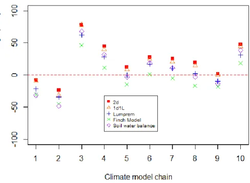
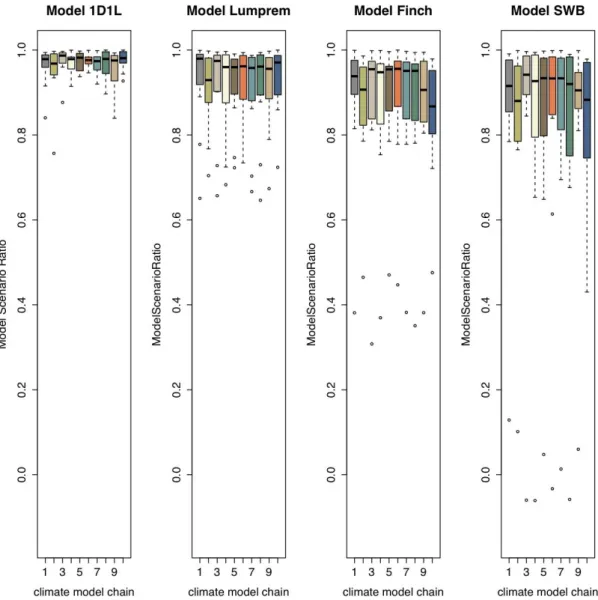
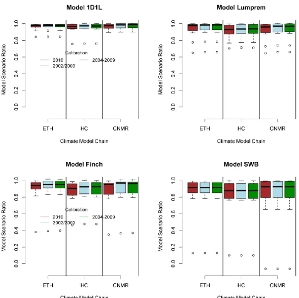
Figure 3. 6: Deviations between mean annual recharge from the baseline (past mean recharge) and for the period 2035 for 10 model chains. 70 Figure 3.7: Model scenario ratio (Equation 13-15) for simplified groundwater

recharge models for each climate model chain. 71

Figure 3. 8: Variations of NSE-Coefficient and PBIAS for different groundwater recharge models. ETHZ_HadCM3Q0_CLM climate model chain is used for the

periods 2035, 2060 and 2085. 73

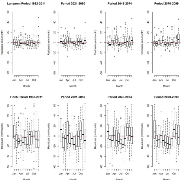
Figure 3. 9: Residuals between simulated monthly Recharge from the reference 2D model and the Lumprem (upper panel) as well as the Finch Model (lower panel)

for the four simulated time slices. 74

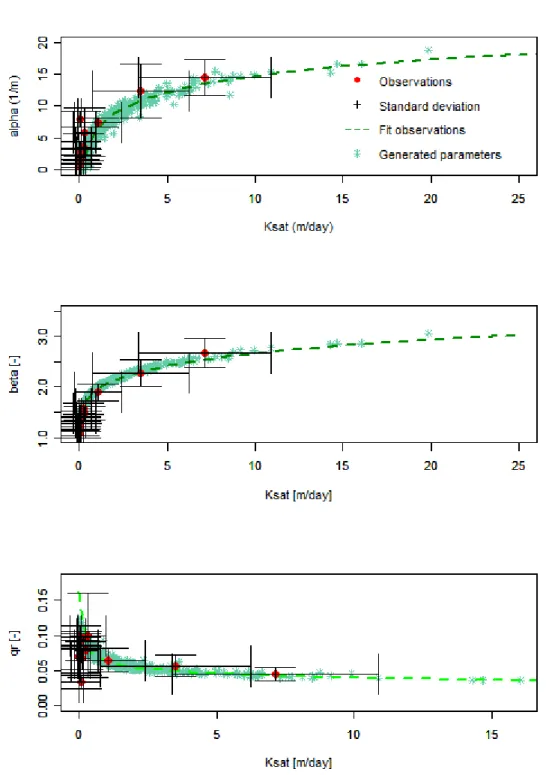
Figure 3. 10: Comparison between the archived MSR for each simplified model under the calibration period 2010 (brown color), 2002/2003 (light-blue color) and 2004-2009(green color) are shown for three model chains. 75 Figure A3. 1: Relationship of the van Genuchten parameters alpha, beta and residual

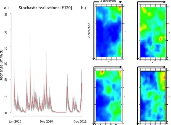
water content (qr) with saturated hydraulic conductivity (Ksat). 84 Figure A3. 2: a.) Daily recharge pattern (mm/day) for year 2010 and 2011 for 130

stochastic hydraulic parameter fields used in the references 2D field. The red line shows the mean recharge from all 130 simulations whereas the gray lines display the variations b.) Four hydraulic conductivity fields from the 130 stochastic

(19)

13

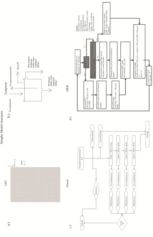
Figure A3. 3: Structure of simplified models for a.) 1D homogeneous soil structure with 1layer (1d1l), b.) Semi-mechanistic model (Lumprem), c.) Soil water balance model with 4 layers and root distribution (Finch) and d.) Simple 1 soil column model without runoff, interception or direct recharge (SWB). 86 Figure A3. 4: Daily recharge pattern for all applied recharge models for the year

2010. 87

Figure A3. 5: Deviations between upper (left panel) and lower (right panel) annual recharge from the baseline (past mean recharge 30 years) and for the period 2035

for 10 model chains. 87

Figure 4. 1: Lysimeter facility surface (a.) and basement (b.) as well as the three

present soil types (c-e). 95

Figure 4.2: Lysimeter data with recharge (mm/h), precipitation (mm/h), mean soil moisture content (SMC in Vol%) and calculated ETa (mm/h) for lysimeter 3 with

the soil type Cambisol. 98

Figure 4.3: Soil moisture content (SMC) for lysimeter 3 in 4 different depths for the entire time series (left panel) and a chosen time slot where differences in SMC

occur (right panel). 99

Figure 4.4: Hourly (left panel) and cumulative seepage (right panel) for lysimeter 3 for the entire time series (top row) and a chosen time slot (bottom row). 100 Figure 4. 5: Daily climatic change factors (Delta-Change Approach) for each climate

model chain for the scenario A1B. a.) Daily precipitation and b.) Daily mean temperature from Meteoswiss weather station in Zurich-Reckenholz. 102 Figure 4. 6: Linear delta change factor interpolation between the year 2011 and the

three-time period 2035, 2060 and 2085 (red lines) for a.) Temperature and b.) Precipitation for each year from 2011 to 2085 and each day is shown. Red and blue colors indicate an increase and decrease trend, respectively. 103 Figure 4. 7 :Fit between measured (grey) and simulated (blue) soil moisture content (SMC) (top row), cumulative seepage (middle row) and cumulative ETa (bottom row) for Winter barley, Phacelia, Sugar beets and Feed wheat for lysimeter 3. The vertical gray line distinguish between calibration and validation period

110 Figure 4. 8: Boxplot summary of all simulations for each crop type and lysimeter as

well as climate model chain and 10 stochastic realisations for 2085 is shown (Period from 2011 to 2085). The percentile change compared to the baseline (past recharge) is displayed. A positive value indicates a recharge increase and a negative a decrease compared to the baseline. The different colours of each boxplot represent the seven different GCM-RCM combinations. 115 Figure 4. 9: Absolute change in recharge rate from the reference period for each

chosen lysimeter and associated crop types. The vertical arrows show the combined uncertainty originated from GCM-RCM combinations and stochastic realisation of the interannual variability in precipitation and temperature. The size of the rectangle shows the model parameter value Leaf area index (LAI) for the related crop, whereas the position indicate the mean simulated change out of

(20)

14

the different from GCM-RCM combinations and stochastic realisation. The

horizontal arrows show the growing period. 116

Figure 4. 10: Absolute change in recharge rate from the reference period for each chosen lysimeter and associated crop types. The vertical arrows show the combined uncertainty originated from GCM-RCM combinations and stochastic realisation of the interannual variability in precipitation and temperature. The size of the rectangle shows the model parameter value root depth (RD) for the related crop, whereas the position indicate the mean simulated change out of the different from GCM-RCM combinations and stochastic realisation. The

horizontal arrows show the growing period. 117

Figure 4. 11: Cumulative seepage water amount between 2011 and 2085 of the transient CC simulation for a.) Temporary grassland, b.) Colza and c.) Feed wheat during their specific vegetation period is shown. The dashed black line represents the baseline (past recharge) whereas the coloured solid lines displayed the seven different GCM-RCM combinations with the associated equiprobable

stochastic realisations. 120

Figure 4. 12: Sensitivity of recharge rates on the Feed wheat a.) LAI and b.) RD. In the references scenario (“original” LAI or RD) LAI and RD corresponds to the original literature values. The red dashed line corresponds to the past recharge rates (baseline). A RD increase for Feed wheat could not be simulated because the actual RD already reaches the bottom depth of the lysimeter. 122 Figure A4. 1: Cumulative seepage water amount between 2011 and 2085 of the transient CC simulation for crops on lysimeter 3 and 5 during their specific vegetation period is shown. The dashed black line represents the baseline (past recharge) whereas the coloured solid lines displayed the seven different GCM-RCM combinations with the associated equiprobable stochastic realisations. 131 Figure A4. 2: Cumulative seepage water amount between 2011 and 2085 of the

transient CC simulation for crops on lysimeter 9 and 10 during their specific vegetation period is shown. The dashed black line represents the baseline (past recharge) whereas the coloured solid lines displayed the seven different GCM-RCM combinations with the associated equiprobable stochastic realisations 132 Figure 5. 1: Schematic simplified geological plane view and cross-sections of the

Wohlenschwil catchment (modified from geological map). 136 Figure 5. 2: a.) Model geometry with finite element model mesh and geological units b.) Calibrated hydraulic conductivity (Ksat m/day) distribution for the sand-gravel aquifer based on the pilot point calibration approach. 140 Figure 5. 3: Ensemble means (red dashed line) and uncertainty ranges (gray shaded area) of daily climatic change factors for 10 GCM-RCM combinations of the A1B scenario. Left column show changes in daily precipitation and right column in daily mean temperature for the time period 2035, 2060 and 2085 for the

Meteoswiss weather station Buchs. 142

Figure 5. 4: Transient calibration of groundwater levels for six piezometers from

(21)

15

Figure 5. 5: Boxplot of annual recharge (mm/a) evaluation for 10 model chains for

time periods a) 2035, b.) 2060 and c.) 2085. 145

Figure 5. 6: Monthly mean recharge rates for the three time periods over 30 years simulation and past conditions (black line). Seasonal decomposition was done for all model chain.5.7.4 Projected change in groundwater level 148 Figure 5. 7: Evolution of the groundwater levels (Water table) at well 96-1 for a.) Period 2035 (2021-2050), b.) Period 2060 (2045-2074) and c.) Period 2085 (2070-2099). The grey shaded line shows the uncertainty range originated from variability among the 10 climate model chains. The black line shows the references period, whereas the green line displays the mean calculated groundwater level based on the simulations under the 10 different climate model

chains. 149

Figure 5. 8: Monthly mean groundwater levels for the three time periods for the past

and future periods. 151

Figure 5. 9: Monthly recharge differences (mm/month) from mean monthly recharge values from the reference period 2012, 360 months) for the a.) Past (1983-2012), b.) Period 2035, c.) Period 2060 and d.) Period 2085. Red lines correspond to the threshold values from the summer heatwave 2003. 152 Figure 5. 10: a.) Probability density function (Kernel density estimates) of recharge differences (mm/month) for past period (grey area), Period 2035 (blue dashed line), Period 2060 (red dashed line) and Period 2085 (green dashed line). The red vertical lines correspond to the threshold values from the summer heatwave 2003. b.) Kernel density estimates of groundwater level differences (m). The Kernel density estimation is a non-parametric way to estimate the probability

density function 154

Figure A5. 1: 24 electrical resistivity profiles in the study area, where dark red colors relates to sand-gravel and blue colors to loam to loamy sand material In the upper panel the location of the 2D sections in the catchment are indicated.

160 Figure A5. 2: Tracer trasnport times, injected mass and assumped flow direction in

the catchement are shown. 161

Figure A5. 3: NaCl tracer concentration over depth used to calculate the drainage rate

with the peak displacement method. 161

Figure A5. 4: Calculated hydraulic conductivity over depth for three locations in the catchment based on Rosetta, a pedo-transfer model, which used the obtained

grain size data. 162

Figure A5. 5: Seasonality of soil moisture content (SMC) in 44cm depth for past conditions and under the ETH climate model chain for period 2035, 2060 and

2085. 162

Figure App1. 1: Flowchart of the methodology to combine pilot point calibration using PEST with HGS. In the top panel, the pre-processing and the preparation of the input files are shown. The lower panel illustrates the calibration procedure.

(22)

16

Figure App1. 2: (a) Distribution of reference hydraulic conductivity [m day-1] within the finite element model domain. (b) Simulated heads within the model domain. 176 Figure App1. 3: Model domain with locations of 12 observation wells (red points), uniformly distributed 130 pilot points (small green points) and constant head

boundary conditions 177

Figure App1. 4: Simulated versus observed heads. Residuals of all observation wells

are displayed in the small rectangle. 178

Figure App1. 5: (a) Reference and (b) calibrated hydraulic conductivity [m day-1]

field within the model domain. 179

Figure App1. 6: Left panel: Influence of observations on predictions (equation 2, see tutorial) by CV. On the x-axis the omitted observation is shown. The predictions, which takes subsequently place are the simulated head produced with parameter values estimated when the chosen observation is omitted. Right panel: The increase of predictive uncertainty variance for each head due to the loss of observation is shown (equation 1, see tutorial). 180 Figure App1. 7: Parameter influence statistics (Equation 1, see tutorial) from the CV experiment. Omitted parameters are labels as observation 1 to 12 as well as observation group top (the 4 observations close to the northern border), down (the 4 observations close to the southern border) and middle (the 4 observations between down and top). All 130 pilot points used in the calibration are displayed at the x-axis. The statistic shows the differences between a calibration with all observation and the re-calibration with omitted observation(s) for the pilot point

(23)

17

List of Tables

Table 2. 1: Summary of the different modeling approaches to estimate groundwater recharge in CC impact studies………..38 Table 3. 1: Percentage changes for the scenario period 2035 (2021-2050) in

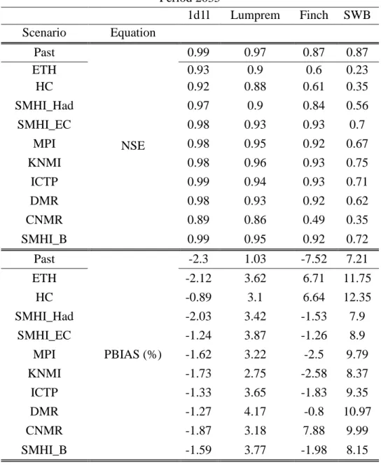
groundwater recharge rates due to variability among the different climate model chains and through different groundwater recharge models………69 Table 3.2: Variation of NSE-Coefficient and PBIAS to different groundwater

recharge models and climate model chains…..………72 Table 3. 3: Variation of NSE-Coefficient and PBIAS to different groundwater

recharge models and climate model chains for calibration period 2010 and

2002/2003 and 2004-2009. ……….77 Table A3. 1: Calibrated model parameter for each recharge model with initial values

and lower as well as upper bound for each calibrated model parameter………..88 Table A3. 2: Climate change scenarios with associated GCMs and RCMs…………89 Table 4. 1: Crop sequences for the five different lysimeters represent three different

soil types. The sowing and harvesting time is given for each crop………..96 Table 4. 2: Table of the used performance criteria to evaluate the fit between

simulated and observed moisture content (MC), seepage water amount and ETa for

each crop and lysimeter. 112

Table 4. 3: Percentage differences in future recharge rates for original crops and with an assumed change from agriculture crop sequence to Temporary grassland for the period 2011-2085. The absolute values indicate the change compared to the baseline (past recharge). ………118 Table 4. 4: Sensitivity of recharge rates to variations in Leaf area index (LAI) and

root depth (RD) for lysimeter 3 and two crops……… 123 Table A4. 1: Vegetation model parameters such as maximum root depth (cm) and

maximum leaf area index (LAI) and transpiration limiting saturation parameters. The calibrated transpiration fitting parameters C1 to C3 are shown as well….130 Table 5. 1: Van Genuchten parameters, residual water saturation, total porosity,

specific storage and saturated hydraulic conductivity. The hydraulic conductivity range for the gravel-sand aquifer is obtained by the calibration. ………. 139 Table 5. 2: Climate change scenarios with associated GCMs and RCMs………… 141 Table 5. 3: Percentage change in mean annual recharge for each climate model chain

and statistics for each time period………. 146 Table 5. 4: Changes in groundwater levels (∆ h) for 2035 (2021-2050), 2060

(2045-2074) and 2085 (2070-2099) for 10 model chains compared to the reference period………..150

(24)

(25)

19

Chapter 1 1.1 Introduction

As highlighted in the Fourth Assessment Report of the Intergovernmental Panel on Climate change (IPCC, 2007) the recently measured increase in global average air and ocean temperatures, the widespread melting of ice and the global average sea level rise are many factors that point towards climate warming. Numerous studies argue that these changes are mostly related to human activities, particularly to the emission of greenhouse gases and aerosols into the atmosphere. An increase in temperature is predicted for most areas in the world. On a global scale, wet climates are becoming wetter and dry climates are becoming drier. Not only the mean climate is expected to change but also extremes such as strong precipitation events and dry spells.

However, these future climate predictions are associated with a large spatial and temporal variation as well as uncertainties. Local climate systems, which can react differently to external forces compared to global systems, are difficult to predict. These climate predictions are affected by several sources of uncertainties. These uncertainties can be due to site-specific reactions caused by topography for example, or the difficulty to predict anthropogenic factors such as greenhouse gas emission trends and land use changes. In addition, the climate system is very intricate as it contains many nonlinear feedback mechanisms such as atmosphere-ocean or atmospheric-dynamic vegetation feedbacks. Some of these relationships are well understood whereas many other are still doubtful. For instance, many small-scale processes such as cloud formation are too small to be represented on the computational grid. However, Stephens (2002) shows how clouds can strongly affect climate change (CC) predictions. This complexity of the climate system makes it very difficult to predict the effect of greenhouse gases and aerosols on the future climate.

Furthermore, when comparing climate model data to observed values, often-systematic errors can be found in variables such as precipitation and temperature, making it necessary to scale and apply correction methods on the data. This bias correction is needed to use the data for hydrological impact studies. In addition to bias correction, there is also a need to downscale results from general climate models (GCM) to regional climate models (RCM) for the investigated catchments to archive the necessary spatial resolution.

However, apart from uncertainties in the predictions and downscaling, observed changes and simulations provide evidence that water resources are potentially affected by CC (IPCC, 2008). CC can modify water availability and water demand.

(26)

20

The combination of decreasing water availability and increasing demand can lead to water shortage. These changes can have consequences for societal, political, economic and ecologic conditions. The United Nations Environment Program about groundwater (UNEP - Morris et al., 2003) mentioned that the contribution from groundwater is vital for water supply. Around two billion people depend directly on aquifers used for drinking water supply. In addition, groundwater is largely used for food production and drinking water supply for almost the half of the largest megacities in the world. In this context of CC, groundwater will likely become more important due to increasing water shortage. This key water source is already under pressure in many regions of the world with a high conflict potential but the conflict potential will certainly still increase due to CC.

Therefore, evaluating the effect of CC on groundwater resources is crucial. Impact studies can indicate how hydrological systems react under CC and are therefore needed and important. A good system understanding and uncertainty projection of CC is always required to make prediction with a high degree of confidence. Only then, policymakers and water managers can develop a sustainable water management strategy.

1.2 Aim and objectives

The project was carried out in the framework of the Swiss national research program on sustainable water management (NRP 61).

The general aim of this PhD study is to increase the understanding of how and to what extent CC affects groundwater systems in Switzerland and influences groundwater availability for water supply. The project focuses on aquifers that are mainly renewed by direct recharge i.e. by infiltration of precipitation through the soil zone. These groundwater systems provide around 40% of drinking water in Switzerland while another 40% originates from aquifers in interaction with rivers. CC effects on alluvial aquifers were investigated in a companion project.

Evaluating CC impacts on groundwater resources raises the question to what extent groundwater recharge will change. Therefore, a major part of this PhD thesis focuses on this topic. Given that for Switzerland, climate models predict more frequent hot and dry summers, while precipitation tends to increase in winter, a special attention was given to possible changes in the seasonal distribution of recharge. The studies mainly considers conditions typically for the Swiss plateau, where most of the population, industrial and agricultural activities are located. In this region, precipitation in form of snow plays only a minor role. Hence, the question of how snow-melt water influences groundwater recharge is not considered in detail in this PhD.

In addition to groundwater recharge, the effect of CC on groundwater levels was explored based on a case study. The main objective of this part was to evaluate if seasonal shifts of groundwater recharge can lead to lower groundwater levels in late

(27)

21

summer and a potential water shortage. Such effects are mainly expected for highly transmissive systems with a low storage capacity that are expected to react rapidly to seasonal variations in recharge. Therefore, a small aquifer consisting of highly permeable glacio-fluvial deposits was selected that is used for water supply for a small town.

When evaluating CC effects on any system, uncertainty is a major challenge due to the strong impact on all predictions. In CC impact studies in hydrology, mainly three sources of uncertainty can be distinguished, uncertainty due to the uncertainty of climate models, the uncertainty due to unknown evolution of land use and society in general, and the uncertainty related to the hydrological models themselves. In this PhD, the role of these three types of uncertainty has received a major attention. Before outlining the research approach in more detail, methods that have previously been used to simulate CC effects on groundwater resources will be reviewed. First, common approaches to simulate future climate conditions will be briefly summarized and downscaling methods (from the global to the local scale), which are relevant for groundwater models, are discussed (Chapter 2.1). Then, a brief overview of expected climate change trends for Switzerland will be given (Chapter 2.2.). A major part of the review (Chapter 2.3) will be dedicated to the analysis of modeling approaches used in previous studies to predict future groundwater recharge and impacts on aquifers. Finally, the role of different types of uncertainties in CC impact studies will be discussed (Chapter 2.4).

(28)

(29)

23

Chapter 2 2.1 General circulation model

GCMs are tools to simulate the climate response to an increase in both greenhouse gas and aerosol concentrations (McGuffie and Henderson- Sellers, 1997). These 3D numerical mathematical models are based on the Navier-Stokes equation. GCMs can cover processes and interplay between the atmosphere, ocean, land surface, snow and ice (Le Treut et al., 2007).

Although GCMs provide geographically distributed and physically consistent predictions of CC, the mesh resolution is frequently around 100-300 km and therefore too coarse for many impact studies. The regional feedback mechanisms are poorly represented for catchment impact studies (Stoll et al., 2011). Downscaling of the GCMs to local/regional scale is therefore required.

Although the GCMs are sophisticated tools for CC studies, any physical process that occurs on scales smaller than the grid of a GCM such as radiation, turbulence or cloud formation must be represented using effective parameters. Distinct parts of the model which describe for instance clouds, cumulus convection, turbulence and surface albedo must be represented with semi-empirical mathematical expressions (McGuffie and Henderson-Sellers, 1997). However, this parameterisation contributes to the model uncertainty (IPCC-TGICA, 2007). Feedback processes such as cloud formation, radiation and snow albedo are another type of uncertainty in the simulations of future climate. For these reasons, GCMs can give different responses to the same forcing depending on how certain processes and feedback are represented (IPCC-TGICA, 2007). Another type of uncertainty originates from the socio-economic scenario. These scenarios are based on a large number of assumptions about global demographics and societal development, energy demand, technologic and economic trends, and corresponding decisions and choices that our world is taking now and may take in the future (IPCC, 2000). In total four storylines, also referred to as pathways, are created to describe the future anthropogenic greenhouse gas emissions (A1, B1, A2 and B2).

In this PhD thesis, only the scenario A1B, which is moderate in terms of CO2 emission increase compared to other scenarios, is used. Only one scenario, the A1B was chosen to lower the computational demand but still representing a reasonable future developing within both extremes, strong increase as well as constant to decrease of greenhouse gas emission (Nakicenovic 2000). The A1B emission scenario is characterized by a balance across technological emphasis between fossil intensive and no fossil energy sources, where balanced is defined as the point where one does not rely too heavily on one particular energy sources. Balance is defined as the point where one does not rely too heavily on one particular energy source. It is assumed that similar improvement rates of all energy supply and end-use technologies arise. The A1B scenario belongs to the A1 scenario family describing a

(30)

24

future world of very rapid economic growth, global population that peaks in mid-century and declines thereafter, and the rapid introduction of new and more efficient technologies (CH2011, 2011).

A temperature increase of 2.1 to 4.5°C with a mean of 3.1 °C is predicted for Switzerland compared to the reference periods 1980-2009 due to the increase in emissions of both gas and aerosol, (Figure 2.1). For comparison, the A2 scenario is described as a “high” radiative forcing scenario with a mean temperature increase of 3.8°C. High radiative forcing scenarios enclose a very heterogeneous world, where a continuous population growth is assumed and technological changes are more fragmented and slower than other storylines. All these assumptions lead to the largest increase in greenhouse gas concentrations of all possible pathways.

Figure 2. 1: The three pathways of anthropogenic greenhouse gas emissions, along with projected annual mean warming for Switzerland for the 30-year average centered at 2085 (aggregated from the four seasons and three representative regions). These pathways are based on assumptions about global demographics and societal development, energy demand, technologic and economic trends, and corresponding decisions and choices that our world is taking now and may take in the future. The unit «CO2eq» is a reference unit by which other greenhouse gases (e.g. CH4) can be expressed in units of CO2. (Figure taken from CH2011 (2011)).

The inter-model spread between the three pathways of anthropogenic greenhouse gas emissions (Figure 2.1, left panel) as well as the variability in the predictions originated by different climate models (right panel; 10 GCM-RCM combinations) in the predicted temperature ranges is shown. All scenarios follow a similar trend between 2011-2020, whereas they deviate increasingly from each other later on. As mentioned earlier, GCMs model runs are time consuming. GCMs are therefore often not run over a complete time series in transient mode but for certain time intervals denoted as time slices or periods.

(31)

25

2.2 Spatial downscaling

Downscaling results from GCMs is needed to obtain the spatial resolution for the investigated catchment scale on a more regional scale. Two downscaling methods are available. (1) statistical-empirical methods such as “Prefect Prog” can be used, which establish relationships between synoptic-scale predictors and local weather conditions, based on observed evidence and transfer relations into the future. (2) “MOS” (Model Output Statics) also known as “weather generators” approach, applies transfer functions to relate simulations to observations. It involves stochastic modeling of (mostly daily) local weather sequences. The advantages of these methods are their cheapness and their efficiency (Stoll et al., 2011). The disadvantages lie in the assumption of a stationary state and in the lack of account for feedback mechanisms. Dynamical downscaling, which implies the use of regional climate models (RCMs), is frequently performed. This methodology implies that a RCM is nested at a higher resolution into a coarse resolution GCM. This is very attractive due to the physically consistent responses. However, limited spatial resolution is given by the RCM, and simulations are computationally expensive. In this process, time-varying large-scale atmospheric fields like wind, temperature and moisture are supplied as lateral boundary conditions. These boundary conditions provide consistent solutions compared to the GCM, but on a sub-grid scale with a more detailed physical description of the orography and land use (CH2011). This process gives the opportunity to generate different GCM-RCM combinations based on different GCM or RCM model parameterisation or structure (CH2011). RCMs can simulate changes in a finer mesh resolution and can take complex topography features, lakes and land cover differences into account. These physically based simulations can improve in respect to GCM output predictions on regional scales (Wang et al. 2004). This is important because land surface feature regulates the regional distribution of climate variables in many regions. However, RCMs are still computationally time expensive and therefore only data for specific scenario periods are available. More comprehensive information about the different approaches and methods can be found in many reviews and research papers (e.g. Wilby and Wigley 1997, Nakicenovic 2000, Fowler et al. 2007, Buser, Kuensch et al. 2009, Buser et al. 2010, Buser, Kuensch et al. 2010, Bosshard et al. 2011, Fischer et al. 2012).

Different model chains were used in this study (stars in Figure 2.2). The chosen GCM and RCM combinations represent a wide range of model structures and assumptions in the model parameterisation. These most reliable model chains are given by the ENSEMBLE project, a project supported by the European commission to develop an ensemble prediction for CC.

(32)

26

Figure 2. 2: Schematic illustration of the utilized model chains of the ENSEMBLE project, all using the A1B emission scenario. Short and long RCM-bars represent simulations that cover the periods 1951–2050 and 1951–2100, respectively. All model chains marked by stars (***) have been used in this PhD. (Figure taken from CH2011 (2011)).

The spatial resolution of the RCMs is, however, still too coarse for the CC impact studies carried out in this PhD thesis. Therefore, additional downscaled data were required, which were provided by the Center for Climate Systems Modeling (C2SM; http://www.c2sm.ethz.ch/). In this study the following two methodologies were used: (1) The so-called delta change approach (Hay et al. 2000, Xu et al. 2005) was used. This method shifts an observed time series by a climate change induced value (Hay et al. 2000). Future weather periods are thus a function of the past climate conditions with added (temperature) or multiplied (precipitation) delta change values (factors). These delta change values are provided for many weather stations in Switzerland for mean temperatures and precipitations (C2SM). Observed time series of both parameters are scaled on a daily basis according to the climate change signal derived from individual GCM-RCM chains. The daily time series of delta change factors for precipitation and temperature covers three periods (2035, 2060 and 2085) relative to the reference period 1980-2009. Details of the methodology are described in Bosshard et al. (2011). This method, however, assumes that the model bias remains constant through time. Furthermore, future interannual variability is not taken into account. The length and numbers of dry or wet spells hence remains unchanged. (2) In addition to the delta change approach, a stochastic weather generator was used (LARS-WG, Racsko et al. 1991, Semenov and Barrow 1997, Semenov et al. 1998) which generates long, synthetic, daily time series of climatic forcing functions. These

(33)

27

simulations are highly related to properties of the observed weather records (Wilby and Wigley 1997). Relationships between daily weather generator parameters and climatic averages for the present period combined with CC signals were established to generate future time series

A combination of the delta change approach with the stochastic weather generator is described in the following. The model chains (GCM-RCM combinations, Figure 2.2) provide a daily time series of delta change factors for precipitation and temperature for three periods (2035, 2060 and 2085) relative to the reference period 1980-2009. In this PhD, these values were combined with the stochastic ‘‘weather generator’’ approach to generate transient climate change scenarios. Linear interpolation was carried out between the three periods with delta change values in order to obtain a continuous time series for each day and each year between 2011 and 2085. These continuous time series of delta change values were subsequently used in a stochastic weather generator (LARS-WG, Racsko et al. 1991, Semenov and Barrow 1997, Semenov et al. 1998) to create possible different realisations of future precipitation and mean temperature values for each of the model chains used for the CC impact studies in this PhD. The different realisations were needed to cover in the most realistic way future possible weather patterns. Using this stochastic approach, it is possible to simulate climate variability. Another advantage of the transient climate change scenarios is that it is possible to analyze in detail the occurrence of expected change. Whereas for the delta change method a recharge increase or decrease can only be predicted for stationary time periods.

The conceptual approach is shown as an example in figure 2.3 for the climate model chain “ETHZ_HadCM3Q0”. The linear interpolation between the years 2011, 2035, 2060 and 2085 for temperature and precipitation for each year from 2011 to 2085 and day during the year is presented.

(34)

28

Figure 2. 3: Linear delta change factor interpolation between the year 2011 and the three time periods 2035, 2060 and 2085 (red lines) for a.) temperature and b.) precipitation for each year from 2011 to 2085 and each day is shown. Red and blue colors indicate increase and decrease trends, respectively.

2.3 Projected climate change for Switzerland

There is strong evidence that climate is changing, as reported in the CH2011 report. The projected increase in temperature for Switzerland follows a similar trend as the trend predicted for Europe (CH2011, 2011). Generally, for southern Europe, a stronger warming is predicted compared to the northern part. For the winter period, a decrease in snow cover is expected for many regions, which intensifies the warming due to lower albedo. In Europe wet climates are becoming wetter and dry climates are becoming drier, which is consistent with the global trend. The climate models indicate that summer temperatures increase more strongly than winter temperatures, and that the warming is slightly more pronounced south of the Alps than in the north. For precipitation amounts, no clear trend between north and south can be shown. Especially for the alpine region, precipitation could either increase or decrease. In this region, predictions of precipitation are quite difficult due to a broad range of mechanisms and microclimates. Due to the fact that studied areas in this project are located in the northern part of Switzerland, changes in precipitation and temperature

(35)

29

of this region will be described in more detail and only a brief description about the changes in the southern part will be given.

Observed and predicted temperatures and precipitations for summer and winter seasons for northern Switzerland show an increasing trend (Figure 2.4) with the three different emission scenarios and selected time periods. For the A1B scenario, the seasonal mean temperature will increase by 2.7-4.1°C until 2100 compared to the reference periods (1980-2009) while the increase is slightly higher (3.2-4.8°C) for the A2 scenario. For the three scenario periods of A1B, an increase in temperature of 0.9–1.4°C by 2035, 2.0–2.9°C by 2060, and 2.7–4.1°C by 2085 is expected (Fischer et al., 2011). Regional and seasonal differences in temperature are relatively small for the first two scenario periods but become more important towards the end of the time series (2100, scenario period 2085). Also, the chosen emission scenario has a weak impact on the predicted changes for the scenario period 2035. However, with increasing time, differences between the emission scenarios in predicted temperature rise.

Trends for precipitation show differences between the summer and the winter. Projected summer precipitation will decrease by 18-24% for the A1B scenario, whereas a 21-28% decrease is predicted for the A1 scenario. Winter precipitation will probably increase, especially in southern Switzerland. However, these predictions are highly uncertain compared to projected changes in temperature. Simulations indicate that an increase in the northern part of Europe is very likely, whereas a decrease in the southern part is predicted. Switzerland is, however, located close to the so-called “transition zone” between these two regimes (CH2011, 2011), implying that uncertainties on the sign of future precipitation changes are large.

No clear trend is seen for all emission scenarios for 2035, but for the subsequent scenario periods, summer precipitation decreases. For the A1B scenario, a decrease in mean precipitation of 10-17% by 2060 and 18-24% by 2085 is predicted (Fischer, Weigel et al. 2012). For the winter period, a small increase is very likely. The decrease in summer precipitation and increase in winter precipitation partly compensate each other with a net decrease of only 10% or less. For southern Switzerland, a bigger change is predicted (an increase of 20% in winter), but the net effect is likely to be more negative compared to the northern part.

(36)

30

Figure 2. 4: Past and future changes in seasonal temperature (°C) and precipitation (%) over northern Switzerland. The changes are relative to the reference period 1980–2009. The thin colored bars display the year-to-year differences with respect to the average of observations over the reference period; the heavy black lines are the corresponding smoothed 30-year averages. The grey shading indicates the range of year-to-year differences as projected by climate models for the A1B scenario (5–95 percentile range for the available model set). The thick colored bars show best estimates of the future projections, and the associated uncertainty ranges, for selected 30-year time-periods and for three greenhouse gas emission scenarios. (Figure taken from CH2011 (2011)).

Together with changes in precipitation and mean temperature, extreme events are also likely to be affected by CC. More frequent and longer warm spells and heat waves are expected. The length of dry spells will also probably increase (BUWAL 2004). During the last decades, the frequency and duration of heat waves have already substantially increased over central Europe including Switzerland (Frich et al. 2002, Della-Marta et al. 2007, Anagnostopoulou and Tolika 2012, Fernandez-Montes and Rodrigo 2012, Kostopoulou et al. 2012, Long et al. 2012, Buishand et al. 2013, Nemec et al. 2013). Schär et al. (2004) point out that by the end of 2100, every second summer could be as warm as the well acknowledged European summer heatwave of 2003 (Stott et al. 2004, Orsolini and Nikulin 2006, Olita et al. 2007, Schiaparelli et al. 2007, Wegner et al. 2008, Trigo et al. 2009, Munari 2011). Many other studies confirm this finding (e.g. Beniston 2007, Beniston 2007, Beniston and Goyette 2007, Beniston et al. 2007, Beniston 2009, Beniston 2013, Fischer et al. 2007, Vidale et al. 2003, Lenderink et al. 2007).

The prediction of frequency and intensity of heavy precipitation events is quite difficult and highly uncertain. However, in the past, an increase in heavy precipitation events was observed in Switzerland (Beniston 2006, Hohenegger et al.

(37)

31

2008, Jaun et al. 2008). Once again it is very likely that the frequency, duration and intensity of both wet and dry extremes changes under CC.

A conceptual scheme, which tries to merge the aforementioned findings for extreme events for the past, together with the actual weather and future predictions is illustrated in figure 2.5. Potential changes in frequency and intensity of temperature and precipitation extremes in a changing climate are shown (dashed lines are used to present the future distribution). Changes in the distribution of temperature and precipitation (mean, variability and shape) might lead to changes in the frequency and intensity of hot, cold, wet and dry extremes.

Figure 2. 5: Illustration of potential changes in frequency and intensity of temperature and precipitation extremes in a changing climate. Current and potential future distributions are depicted with full and dashed lines, respectively. Changes in the distribution of temperature and precipitation (mean, variability and shape) potentially lead to changes in the frequency and intensity of hot, cold, wet and dry extremes. (Figure modified from CCSP 2008).

2.4 Climate Change and Hydrology

The aim of this section is not to provide a complete picture about CC and hydrology but rather to summarise the main aspects of this wide research field.

It is indisputable that the evaluation of the effect of climate change on water resources is essential for a successful water management under future climate conditions. Changes in precipitation patterns and amounts as well as increases in mean temperatures can have a significant impact on all components of the hydrological cycle. Changes in

 river discharge (Eckhardt and Ulbrich 2003, Scibek 2007, Serrat-Capdevila and Valdes et al., 2007, van Roosmalen et al., 2007, Woldeamlak et al., 2007, Goderniaux et al., 2009, Mileham et al., 2009, van Roosmalen et al., 2009, Kingston and Taylor 2010, van Roosmalen et al., 2010, Gosling et al., 2011, Kingston et al., 2011, Velázquez et al., 2013, Barthel 2011, Barthel 2011, Barthel et al., 2011, Barthel et al., 2011, Todd et al., 2011, van Roosmalen et

(38)

32

al., 2011, Barthel et al., 2012, Gosling et al., 2012, Sonnenborg et al., 2012, Thompson et al., 2013),

 surface runoff (Woldeamlak et al.. 2007, Mileham et al., 2008, Mileham et al., 2009, Gosling et al., 2011, Barthel et al., 2012, Gosling et al., 2012, Bush et al., 2010, Gosling 2013, Seidel and Martinec 2004, Furher et al,. 2013, Alaoui et al., 2013, Chiew et al., 1995),

 groundwater recharge (Holman 2006, Holman 2006, Scibek 2006, Serrat-Capdevila et al., 2007, van Roosmalen et al., 2007, Woldeamlak et al., 2007, Barthel et al., 2008, Mileham et al., 2008, Goderniaux et al., 2009, van Roosmalen et al., 2009, Barthel et al., 2010, Kingston and Taylor 2010, van Roosmalen et al., 2010, Barthel 2011, Barthel 2011, Barthel et al., 2011, Barthel et al., 2011, Stoll et al., 2011, van Roosmalen et al., 2011, Barthel et al., 2012, McCallum et al., 2010, Crosbie et al., 2011, Crosbie et al., 2012, Thampi and Raneesh 2012, Crosbie et al., 2013),

 snowpack (Graham et al., 2007, Seidel and Martinec 2004, Andréasson et al., 2004, Wilby et al., 2008, Benistion 1997, Benistion et al., 2003, Furher et al., 2013, Alaoui et al., 2013),

 and soil moisture content (Asiedu et al., 2013, Rodriguez‐Iturbe 2000, Laio et al., 2001, Chiew et al., 1995, Seneviratne et al., 2010, Fischer et al., 2007) can occur. An excellent review can be found in Green et al. (2011) and a summary of recommendations on how to deal with CC and groundwater is presented in Holman et al. (2012).

The majority of CC impact studies focus on surface water. Although groundwater has received more attention in the past years (Green et al., 2011), there is still little known about the sensitivity of groundwater to CC compared to surface water. The often slow response of groundwater to changes in the climatic forcing functions due to CC compared to surface water can be an explanation. The significance of impact studies dealing with CC and groundwater is perhaps less noticed.

A major requirement in CC impact studies is a good knowledge about groundwater recharge. Quantification is needed because for any robust model prediction, groundwater recharge is one of the main drivers of the hydrological system. This applies not only to groundwater studies but also to surface water as baseflow directly depends on the renewal of groundwater resources.

Further trends in groundwater recharge are directly related to the predicted changes in temperature and precipitation due to an increase in greenhouse gas concentrations. However, it is unlikely to assume that societal, political and economic conditions will remain unchanged in the future and that only climate change will be the driving force for changes in recharge rate (Holman et al., 2012). Land use will likely change which has a direct impact on the water balance (e.g. Holman 2006, Keese et al., 2005, Eitzinger et al., 2003).

For predictions of CC impacts on water resources, mathematical models are essential. These models provide insight into the response of groundwater systems to CC (Green