Understanding and Guiding the Computing Resource Management in a Runtime Stacking Context

HAL Id: tel-02438652

https://hal.inria.fr/tel-02438652

Submitted on 14 Jan 2020

HAL is a multi-disciplinary open access

archive for the deposit and dissemination of sci-entific research documents, whether they are pub-lished or not. The documents may come from teaching and research institutions in France or abroad, or from public or private research centers.

L’archive ouverte pluridisciplinaire HAL, est destinée au dépôt et à la diffusion de documents scientifiques de niveau recherche, publiés ou non, émanant des établissements d’enseignement et de recherche français ou étrangers, des laboratoires publics ou privés.

Management in a Runtime Stacking Context

Arthur Loussert

To cite this version:

Arthur Loussert. Understanding and Guiding the Computing Resource Management in a Runtime Stacking Context. Distributed, Parallel, and Cluster Computing [cs.DC]. Université de Bordeaux, 2019. English. �tel-02438652�

PRÉSENTÉE À

L’UNIVERSITÉ DE BORDEAUX

ÉCOLE DOCTORALE DE MATHÉMATIQUES ET

D’INFORMATIQUE

par Arthur Loussert

POUR OBTENIR LE GRADE DE

DOCTEUR

SPÉCIALITÉ : INFORMATIQUE

Understanding and Guiding the Computing

Resource Management in a Runtime Stacking

Context

Rapportée par :

Allen D. Malony,Professor , University of Oregon

Jean-François Méhaut, Professeur , Université Grenoble Alpes

Date de soutenance : 18 Décembre 2019

Devant la commission d’examen composée de :

Raymond Namyst, Professeur , Université de Bordeaux – Directeur de thèse

Marc Pérache,Ingénieur-Chercheur , CEA – Co-directeur de thèse

Emmanuel Jeannot, Directeur de recherche, Inria Bordeaux Sud-Ouest – Président du jury Edgar Leon, Computer Scientist , Lawrence Livermore National Laboratory – Examinateur

Patrick Carribault, Ingénieur-Chercheur , CEA – Examinateur

Julien Jaeger, Ingénieur-Chercheur , CEA – Invité

ment

Abstract With the advent of multicore and manycore processors as building blocks of HPC supercomputers, many applications shift from relying solely on a distributed programming model (e.g., MPI) to mixing distributed and shared-memory models (e.g., MPI+OpenMP). This leads to a better exploitation of shared-memory communications and reduces the overall memory footprint. However, this evolution has a large impact on the software stack as applications’ developers do typically mix several programming models to scale over a large number of multicore nodes while coping with their hiearchical depth. One side effect of this programming approach is runtime stacking: mixing multiple models involve various runtime libraries to be alive at the same time. Dealing with different runtime systems may lead to a large number of execution flows that may not efficiently exploit the underlying resources.

We first present a study of runtime stacking. It introduces stacking config-urations and categories to describe how stacking can appear in applications. We explore runtime-stacking configurations (spatial and temporal) focusing on thread/process placement on hardware resources from different runtime libraries. We build this taxonomy based on the analysis of state-of-the-art runtime stacking and programming models.

We then propose algorithms to detect the misuse of compute resources when running a hybrid parallel application. We have implemented these algorithms inside a dynamic tool, called the Overseer. This tool monitors applications, and outputs resource usage to the user with respect to the application timeline, focusing on overloading and underloading of compute resources.

Finally, we propose a second external tool called Overmind, that moni-tors the thread/process management and (re)maps them to the underlying cores taking into account the hardware topology and the application behav-ior. By capturing a global view of resource usage the Overmind adapts the process/thread placement, and aims at taking the best decision to enhance the use of each compute node inside a supercomputer. We demonstrate the relevance of our approach and show that our low-overhead implementation is able to achieve good performance even when running with configurations that would have ended up with bad resource usage.

Host Laboratory:

CEA, DAM, DIF, F-91297 Arpajon, France Inria Bordeaux Sud-Ouest

Mots-clés Calcul Haute Performance, Programmation Parallèle, MPI, OpenMP, Mélange de Modèles de Programmation, Allocation des Ressources, Gestion des Ressources

Résumé La simulation numérique reproduit les comportements physiques que l’on peut observer dans la nature. Elle est utilisée pour modéliser des phénomènes complexes, impossible à prédire ou répliquer. Pour résoudre ces problèmes dans un temps raisonnable, nous avons recours au calcul haute per-formance (High Perper-formance Computing ou HPC en anglais). Le HPC regroupe l’ensemble des techniques utilisées pour concevoir et utiliser les supercalcula-teurs. Ces énormes machines ont pour objectifs de calculer toujours plus vite, plus précisément et plus efficacement.

Pour atteindre ces objectifs, les machines sont de plus en plus complexes. La tendance actuelle est d’augmenter le nombre cœurs de calculs sur les processeurs, mais aussi d’augmenter le nombre de processeurs dans les machines. Les ma-chines deviennent de plus en hétérogènes, avec de nombreux éléments différents à utiliser en même temps pour extraire le maximum de performances. Pour pallier ces difficultés, les développeurs utilisent des modèles de programmation, dont le but est de simplifier l’utilisation de toutes ces ressources. Certains modèles, dits à mémoire distribuée (comme MPI), permettent d’abstraire l’en-voi de messages entre les différents nœuds de calculs, d’autres dits à mémoire partagée, permettent de simplifier et d’optimiser l’utilisation de la mémoire partagée au sein des cœurs de calcul.

Cependant, ces évolutions et cette complexification des supercalculateurs à un large impact sur la pile logicielle. Il est désormais nécessaire d’utiliser plusieurs modèles de programmation en même temps dans les applications. Ceci affecte non seulement le développement des codes de simulations, car les développeurs doivent manipuler plusieurs modèles en même temps, mais aussi les exécutions des simulations. Un effet de bord de cette approche de la programmation est l’empilement de modèles (‘Runtime Stacking’) : mélan-ger plusieurs modèles implique que plusieurs bibliothèques fonctionnent en même temps. Gérer plusieurs bibliothèques peut mener à un grand nombre de fils d’exécution utilisant les ressources sous-jacentes de manière non optimale. L’objectif de cette thèse est d’étudier l’empilement des modèles de program-mation et d’optimiser l’utilisation de ressources de calculs par ces modèles au cours de l’exécution des simulations numériques. Nous avons dans un premier temps caractérisé les différentes manières de créer des codes de calcul mélan-geant plusieurs modèles. Nous avons également étudié les différentes interactions que peuvent avoir ces modèles entre eux lors de l’exécution des simulations.

outil permettant de diriger automatiquement l’utilisation des ressources par les différents modèles de programmation.

Pour illustrer les différentes techniques permettant de mélanger plusieurs modèles de programmation dans un code de calcul, ainsi que les interactions possibles, nous avons introduit des configurations et catégories de mélange. Cette taxonomie est la base des travaux de cette thèse ainsi que sa première contribution. Les catégories définissent comment des situations de mélange de modèles peuvent être créées. Elles illustrent également l’influence que peuvent avoir les développeurs sur ces modèles à l’exécution. En effet, certaines tech-niques de programmation laissent les programmeurs décrire tous les appels aux modèles de programmation. Dans ce cas, c’est aux utilisateurs des applications de gérer tous les paramètres de ces modèles. Il est possible d’optimiser ces paramètres en fonction de l’application, de la machine, des besoins etc. Des erreurs d’optimisation sont aussi possible, car il faut gérer un très grand nombre de paramètres, et ces paramètres peuvent changer en fonction de l’architecture de la machine, etc. De l’autre cote du spectres, certains langage de program-mation font une totale abstraction des modèles et gèrent les ressources sans que l’utilisateur n’ait a faire quoi que ce soit. Dans ce cas, les possibilités d’optimisation sont moindres, mais c’est aussi le cas des possibles erreurs. De ces catégories ressortent plusieurs points importants. Le premier est qu’il existe un grand nombre de techniques différentes permettant de créer des codes de calcul utilisant plusieurs modèles de programmation. Chacune a ses avantages et inconvénients, selon l’application, la machine, les utilisateurs etc. La seconde est qu’il n’existe pas de solution miracle pour toutes ces plateformes de pro-grammation, il existe trop de modèles et techniques. De ce fait, nous avons dû dans la suite de cette thèse, nous raccrocher au bloc de base de ces modèles : ils utilisent tous des processus et processus légers. C’est le point d’entrée que nous avons utilise pour étudier et optimiser l’utilisation des ressources par tous ses différents modèles de programmation.

La seconde partie de la taxonomie définit les possibles interactions entre les mo-dèles de programmation pendant l’exécution des simulations. Ces interactions sont découpées en deux configurations : les interactions spatiales et temporelles. Si deux modèles sont spatialement concurrents par exemple, il est possible qu’ils se disputent des ressources de calcul. Deux modèles spatialement indépendants peuvent aussi interagir entre eux, s’ils sont temporellement concurrents et qu’ils s’envoient des messages par exemple. Les configurations de mélange nous informent sur les éventuels interactions entre modèles. De plus, connaitre la configuration des modèles permet aussi de concentrer les efforts d’optimisations sur les problèmes réellement rencontrés.

mé-sur les processus et processus légers, mais aussi mé-sur quel type d’erreur nous focaliser. Suite a la création de cette taxonomie, nous avons également remarque qu’aucun outil d’aide au développement ne prenait en compte le mélange de programmation. Commettre une erreur dans les paramètres des modèles ne soulève aucune erreur ou avertissement à la compilation, et il en est de même pour une mauvaise utilisation des ressources à l’exécution. De ce fait, nous avons décidé de nous pencher sur l’utilisation des ressources par les modèles de programmation.

La seconde contribution de cette thèse est une suite d’algorithmes per-mettant de détecter les possibles mauvaises utilisation de ressources par les processus et processus légers. Ces algorithmes restent centrés autours des pro-blématiques liées aux modèles de programmation. Ils se basent sur des traces d’exécution, contenant des indices sur le placement des fils d’exécution sur les ressources. En utilisant ces informations, ils déterminent si certaines ressources ont pu être surchargées ou non utilisées par exemple. Nous avons implémenté ces algorithmes dans un outil d’analyse pour aider à l’optimisation des codes de calcul. La première étape est de récolter les informations sur le placement des fils d’exécution. Pour ce faire, nous avons développé une bibliothèque dyna-mique qui récolte toutes les informations nécessaire pendant l’exécution des applications. Cette bibliothèque apporte un très faible surcout en temps, et ne nécessite aucun changement dans le code ou la chaine de compilation de l’application ciblée. Une fois les informations récoltés, nous pouvons utiliser nos algorithmes. Ceux-ci fournissent un rapport décrivant l’utilisation des ressources par les fils d’exécution. Ce rapport permet de déterminer si un changement dans les paramètres des modèles de programmation peut être bénéfique pour les performances de l’application. Cependant, même si cet outil peut donner des indices sur les améliorations et optimisations possibles, il reste toujours un très grand nombre de paramètres à connaitre et modifier pour optimiser une application.

La troisième contribution de cette thèse est second un outil, aillant pour objectif de placer dynamique les fils d’exécution sur les ressources de calcul. Il utilise les développements et informations récoltés par ce premier outil pour déterminer dynamiquement un placement en fonction des fils d’exécution en présence ainsi que l’architecture de la machine. Cet outil n’est encore qu’une preuve de concept, mais il présente des résultats encourageants pour la suite. Nous avons tout d’abord observé que la grande majorité des codes de simulation utilisent MPI pour gérer les communications entre les nœuds de calculs. Parfois, un modèle à base de processus légers est ajouté pour optimiser l’utilisation de la mémoire partagée sur les nœuds. Dans ce type de configuration,

l’optimisa-un maximum de ressources pour leurs calculs et les processus légers partageant de la mémoire sont regroupes sur les mêmes mémoires physiques. Nous avons utilisé cette heuristique pour développer notre outil. Les tests que nous avons effectués montrent que cette heuristique produit les meilleurs résultats sur les applications utilisées de nos jours sur les supercalculateurs. Utiliser notre outil permet de minimiser les erreurs de placement de modèles de programmation. Dans le futur, nous souhaitons développer de nouveaux algorithmes pour cet outil. Ceux-ci apporteraient une plus grande flexibilité et permettraient d’adap-ter notre outil à des applications présentant des comportement différents de ceux observes jusqu’à maintenant.

En conclusion, cette thèse apporte un regard sur une problématique impor-tante du calcul haute performance : l’empilement de modèles de programmation. Avec l’évolution des architectures des supercalculateurs, cette problématique risque de devenir de plus en plus importante pour les performances des codes de calcul. Cette thèse propose une taxonomie permettant de décrire les tech-niques menant à l’empilement de modèles ainsi que les potentiels problèmes qui peuvent survenir à l’exécution. Nous avons également développé des algo-rithmes permettant de détecter les mauvaises utilisations de ressources sur les supercalculateurs. Ces algorithmes ont été implémentés dans un outil d’aide à l’optimisation. Nous avons également développé un second outil permettant de gérer dynamiquement les fils d’exécution et les ressources pendant l’exécution de codes de calcul. Toutes ces contributions sont centrées sur les modèles de programmation et prennent en compte des problématiques qui leur sont propres. Plusieurs pistes d’amélioration sont envisagées pour nos différents outils : • Les deux outils développés sont toujours au stade de preuve de concept.

Nous souhaitons ajouter des paramètres pour leur donner une vision plus large des problèmes de gestion de ressources. Nous nous sommes pour l’instant focalisés sur les processus et processus légers ainsi que les cœurs de calcul. Il est envisageable d’étudier d’autres ressources comme la mémoire par exemple. De plus, les futures architecture risquent d’exposer de plus en plus d’hétérogénéité. Certains cœurs de calculs pourraient par exemple être spécialisés dans les communications entres nœuds. Dans ce cas, placer le fils d’exécution effectuant les communications sur le cœur approprié serait une optimisation intéressante pour les performances. Nos outils doivent donc évoluer et prendre en compte les problématiques futures.

• Nous nous sommes aussi focalisés sur un type d’application particulier. Ce type d’application correspond à la grande majorité des codes de calculs utilisés sur supercalculateurs mais cela pourrait évoluer. Dans certains cas,

nous avons pour objectif de développer un langage simple permettant à un utilisateur de décrire ses besoins. Grâce a cette description, nos outils pourraient prendre les meilleurs décisions pour coller aux besoins des utilisateurs.

Dans un contexte plus large, cette thèse est centrée sur ce qu’il se passe quand une application utilise plusieurs modèles de programmation. Cependant, un supercalculateur fait rarement une seule simulation, plusieurs sont en cours en même temps. De ce fait, nous pensons qu’élargir les problématiques d’empi-lement de modèles au gestionnaire de ressource pourrait être bénéfique. Celui-ci pourrait par exemple utiliser les périodes creuse des applications pour effectuer des travaux légers. Ceci améliorerait le rendement des supercalculateurs en augmentant leur taux d’utilisation et en diminuant les pertes d’énergie. Laboratoires d’accueil :

CEA, DAM, DIF, F-91297 Arpajon, France Inria Bordeaux Sud-Ouest

Contents ix

1 Introduction 1

I

Context and State-of-the-Art

5

2 Computer Hardware and Software Evolution 7

2.1 Computer architecture: From single-core to actual multi and

many-cores . . . 7 2.1.1 Moore’s Law. . . 8 2.1.2 Clock speed . . . 9 2.1.3 Parallelism Advent . . . 12 2.1.4 Instruction-Level Parallelism . . . 13 2.1.4.1 Pipelining . . . 14 2.1.4.2 Hazards in pipelines . . . 16

2.1.4.3 Conclusion on Instruction Level Parallelism . . 17

2.1.5 Thread level parallelism . . . 18

2.1.5.1 Multicore Architectures . . . 18

2.1.5.2 Memory Hierarchy . . . 19

2.1.5.3 Non Uniform Memory Access (NUMA) . . . 22

2.1.6 Data level parallelism in vector and manycores . . . 23

2.1.6.1 Vector Architecture. . . 23

2.1.6.2 Manycore architectures. . . 23

2.1.7 Conclusion on evolutions . . . 24

2.2 Supercomputer Architecture . . . 24

2.2.1 Supercomputers Tops . . . 24

2.3 Parallel programming models . . . 26

2.3.1 Shared-memory models . . . 28

2.3.1.1 POSIX Threads. . . 28

2.3.1.2 OpenMP standard . . . 30

2.3.1.3 Shared-memory models conclusion . . . 31

2.3.2.1 Message Passing Interface (MPI) . . . 31

2.3.2.2 Distributed-memory model conclusion . . . 32

2.3.2.3 Hybrid programming . . . 32 2.4 Conclusion . . . 33 3 Problem 35 3.1 Motivating Example . . . 36 3.2 Contributions . . . 38

II

Contributions

39

4.3.1 Explicit addition of runtimes. . . 48

4.3.1.1 Intra-application . . . 48

4.3.1.2 Inter-application . . . 50

4.3.2 Implicit use of runtimes . . . 50

4.3.2.1 Direct addition . . . 50

4.3.2.2 Indirect addition . . . 52

4.3.3 Discussion . . . 52

4.4 Taxonomy conclusion . . . 53

5 Algorithms and Tools 55 5.1 Bibliography. . . 56

5.2 Algorithms detecting resource usage. . . 56

5.3 Tool producing logs . . . 60

5.3.1 Other trace possibilities . . . 61

5.4 Putting it all together: analysing logs and producing warnings . 63 5.5 Experimental Results . . . 64

5.5.1 Test bed description . . . 64

5.5.2 Tool overhead . . . 65

5.5.3 Benchmark Evaluation . . . 65

5.5.4 Improving analysis with temporal information . . . 70

6 Hypervising Resource Usage 75

6.1 Bibliography. . . 75

6.2 Overmind’s Design . . . 77

6.3 Thread management Algorithm . . . 79

6.4 Overmind’s Implementation . . . 81 6.4.1 Information Gathering . . . 81 6.4.2 Worker Placement. . . 82 6.5 Experimental Results . . . 83 6.5.1 Overmind Overhead . . . 83 6.5.2 Benchmark Evaluation . . . 84

6.6 Conclusion and Discussion . . . 87

6.6.1 Conclusion. . . 87

6.6.2 Discussion . . . 87

III

Conclusion and Future Work

89

7.2 Contributions’ Perspectives . . . 92

Introduction

Numerical simulation is the reproduction of real, physical behavior using computers and the tremendous computing power assiociated with them. It is used to model complex phenomena, otherwise impossible to replicate or predict. It has become an essential tool in the industry as it can reduce the cost of expensive experiments. Numerical simulation is for example present in engineering design. Automotive industry relies on simulation to design cars and perform thousands of crash-test experiments without having to build multiple expensive prototypes. The same principles apply to wind tunnel experiments performed by automotive and aerospace industry to optimize aero dynamics of a car, plane wings, or a space rocket. Oil and gaz companies reduce risks and costs when drilling for oil. Simulation also helps to predict weather forecast, for financial simulations, by biosciences, and so on. However, simulation is not only used to reduce costs in industry. It is also hugely exploited in research. Recently, reaserchers at Los Alamos Natrional Laboratory simulated an entire gene of DNA, composed of one billion atoms, that will help better understand and develolp cures for deseases like cancer [1]. Earlier, in 2012, the DEUS consortium managed to simulate the structure of the observable universe since the Big Bang [2]. Scientists from both Research and Industry perform these simulations using the most powerful computers in the world, called supercom-puters. These specialised machines are designed to provide as much computing performances as possible. The science and techniques related to the design and exploitation of these computing beasts is called High Performance Computing (HPC).

Supercomputers are more complex to exploit than traditional desktop com-puters. Two major factors are to take into account. First, supercomputers are composed of multiple inter-connected machines, and second, they are composed of high-performance processors. Let us focus on each factor independantly.

mance, the codes need to be designed in a way that they can be split into pieces, performed in parallel. These parts sometimes need to communicate with each other to update data and move the simulation forward. All these constraints on code parallelism require new programming methods. Parallel algorithms first, but also standards to help with communications. The most widespread standard for parallel programming is called Message Passing Interface [3] (MPI).

Supercomputers are using high performance processors. This perfor-mance comes from the large number of compute cores. The Intel KNL is for example composed of 72 cores accessing some shared-memory. Exploiting shared-memory also requires dedicated techniques, to avoid non-deterministic results. Standards exist to help with this side of the programming too. The most widespread model for shared-memory exploitation in HPC is certainly OpenMP [4]. Finally, to always provide more compute power, heterogeneous components are added to already complex architectures. Some are specialised in certain kind of parallelism, for specific simulations. In the future we will certainly see heterogeneous processors, with some core specialised in communi-cations, some in I/O operations, and so on.

Therefore, to exploit supercomputers to their maximum, simulation codes need to rely on multiple programming models standards and their implemen-tations, called runtimes. It creates situations where multiple runtimes may cohabit and share supercomputer resources. We propose to call these situations Runtime Stacking. One issue is that these models were designed independently from one another. Thus, at execution time, they could potentially be unaware of each other, and compete for resources, creating resource misuse and a slow down of applications. With the complexity and specialisation of compute resources, the number of runtimes used in simulation codes is increasing, and with it the probability of resource misuse. Runtime stacking study is therefore necessary to better seize supercomputer compute power and limit performance degradations.

In this context, this thesis proposes a study of runtime staking techniques and effects on application performances. First we focus on the way runtimes can be mixed at execution time. We define runtime stacking configurations to describe how compute instructions from different runtimes share resources spa-tially and temporally. We also identify runtime stacking categories to illustrate the different situations where mixing multiple parallel programming models may appear. From these observations we design and implement algorithms to check the configuration of an HPC application running on a supercomputer.

These algorithms detect misuse of any resource used by the application. We then implement these algorithms in a software tool call the Overseer that not only checks resource usage, but also warns the user in case of misuse. This tool is used to show how runtime placement and resource usage can impact the performances of parallel applications. We then present a new approach to dynamically handle resource assignment in HPC parallel environments. This approach is implemented in the Overmind, a software that catches the creation of compute workers and reorganizes their binding to avoid misuse of resources relying on the previous algorithms.

This document is organized in three parts. The first one is composed of the Chapter2 presenting the context of the thesis and Chapter 3formulating the problem. The context chapter introduces all the basic knowledge needed to understand the document. It presents the evolution of parallel computer architectures as well as techniques to exploit them. The next chapter brings the focus on our problem with a motivating example. The second part of the thesis is composed of its contributions. We first define taxonomies of runtime stacking configurations and categories in Chapter 4. Chapter5 then describes our algorithms to detect the current runtime-stacking configuration and check for resource usage. This chapter also presents and evaluates our implementation of these algorithms in our first tool, the Overseer. Next, Chapter 6describes the design of our second tool, the Overmind. Finally, the last part concludes the document. We summarize our contribution and discuss future work as well as mid and long term perspectives in Chapter 7.

Computer Hardware and Software

Evolution

Since the invention of computers, tremendous changes have happened both in technology and design. As a comparison, a low-budget laptop bought today around $300 with any Intel i3 processor would produce around 2 GFLOPS (i.e., two billion floating-point operations per second). In 1985 the best

super-computer, the Cray-2 peaking at 1.9 GFLOPS, cost more than $10 million. This massive growth came from advances in technologies used to build com-puters and from innovations in computer design. This first chapter introduces basic HPC concepts needed to understand this PhD Thesis. It also presents the evolutions that took place to reach the current supercomputer performances. Section 2.1 is an overview of important computer evolutions that led to supercomputer we use today. The technological and architectural advances are not necessarily presented chronologically as there is too much overlap and fields advancing at the same time. They are thus presented in an almost chronological, convenient order. Section 2.2presents the architecture of current HPC clusters. Section 2.3 then presents an overview of the methods used to exploit these complex architectures.

2.1

Computer architecture: From single-core to

actual multi and many-cores

This section presents the relevant advances related to computer architecture from the very beginning of computers to current massively parallel supercom-puters. All the presented advances are related to microprocessors and how to exploit them. However, showing a clear chronological view of these advents is not practical. In fact, there are two main possibilities to extract more perfor-mances from microprocessors: make them work faster, or add units to process

Figure 2.1.1 – Evolution of Uniprocessor Performance since 1978 [5]

more tasks at once. Advances on both front were conducted concurrently, creating a chaotic timeline to follow. Lastly there was also another solution. This one is not to extract more from microprocessors, but from the machine in general: use more processors. This is also a massively used technique, particularly in HPC machines.

2.1.1

Moore’s Law

The first design of the computer framework dates back to the early/mid 19th century by Charles Babbage. From there, and to even build the first computer, breakthroughs had to happen. In 1949, the concept of integrated circuits appeared. However, we had to wait almost 10 more years to see the first working example of such circuit in September 1958. From there, advances in technology used to build computers and innovations in computer design made possible to deliver performance improvement of about 25% per year.

In 1965 G. E. Moore predicted an increase in the number of transistors on integrated circuit doubling every year. In 1975, he revised the forecast to doubling every two years. This prediction proved accurate for several decades. Figure 2.1.1 presents the actual growth in processor performance since 1978. Performances of processors are relative to the VAX 11/780, a minicomputer introduced in October 1977, the first to implement the VAX architecture and

measured by the SPEC benchmark. We can observe the rapid growth in performances of processors from their creation to the beginning of the third millennium. Then the growth slows a bit each year. We will present the major innovations which made this rapid growth possible, and the limits we reached in the past decades.

When creating the first processors, electronic components could not fit on only one integrated circuit. Thus, multiple circuits had to be connected. The invention of the microprocessor greatly reduced the cost of processing power as well as speed up computations thanks to reduced distances between components. The first iteration of commercialized microprocessor happened in 1971 by Intel with the Intel 4004. This processor was composed of 2300 transistors. From there, the number of transistors on a microprocessor has been constantly rising based on the decreasing size of transistors. Today’s processors incorporate up to 20 millions transistors. In fact, following Moore’s law was possible just by decreasing semiconductor feature size. All these factors also led to a higher rate of performance improvement with an average of around 35% per year. This growth rate as well as mass-produced microprocessors led to important changes: no need for assembly language any more, and vendor independent standardized operating systems like UNIX and later Linux. This in turn made the development of a new set of architectures, with simpler instruction sets pos-sible. The RISC architecture (Reduced Instruction Set Computer), developed in the early 80s, focused on the exploitation of instruction parallelism (initially pipeline) and the use of caches (initially simple then sophistically organised and optimized). This led to 17 years of sustained growth in performances at an annual rate of over 50% as we can see on Figure 2.1.1. This period unfortunately had to end due to multiple factors. Most importantly, process technology (the semiconductor manufacturing process) is at its limits. Indeed, diminishing semiconductor size, the backbone of performance improvement is not as easy any more, if actually possible.

Since 2003 single processor performance improvement has dropped to less than 22% per year due to the twin hurdles of maximum power dissipation of air-cooled chips and the lack of more instruction-level parallelism to exploit efficiently

2.1.2

Clock speed

Concurrently and linked to processor density evolution, another factor in performance growth is the clock rate increase in processors. In their basic oper-ational principles, processors use transistors. These transistors put together form logical gates that can perform operations. The speed at which these operations can be done represent the clock speed of a processor. If we can give

Figure 2.1.2 – Evolution of microprocessor clock rate between 1978 and 2010 [5] 1 10 100 1000 10,000 1978 1980 1982 1984 1986 1988 1990 1992 1994 1996 1998 2000 2002 2004 2006 2008 2010 2012 C lo ck ra te (MH z)

Intel Pentium4 Xeon 3200 MHz in 2003

Intel Nehalem Xeon 3330 MHz in 2010 Intel Pentium III

1000 MHz in 2000 Digital Alpha 21164A

500 MHz in 1996 Digital Alpha 21064 150 MHz in 1992 MIPS M2000 25 MHz in 1989 Digital VAX-11/780 5 MHz in 1978 Sun-4 SPARC 16.7 MHz in 1986 15%/year 40%/year 1%/year

Figure 2.1.3 – Evolution of the processor-memory performance gap starting in the 1980 [6]

our processor 1 input signal and get 1 result (error free) per second, then our processor’s clock rate is 1Hz. For a while, clock speed was the main concern of manufacturers. It’s easy to understand why. By doubling the clock speed of a processor, codes ran two times faster. And this only by changing architecture, nothing had to be done with the code itself.

Now how can clock speed increase? Getting transistors to perform faster has a limit. This limit is the frequency at which the transistors can switch from on to off and off to on. However, a solution to this physical limit is to add more transistors, adding a new physical limit in the equation: space. We can see how Moore’s law comes into account with this first solution: decreasing component size, adding more components, and in the process improving pro-cessor performances. However, since CPUs stay roughly the same size, adding more and more transistors is not possible eternally. In fact, feature size of processors is getting to its physical limit.

Moreover, energy consumption is becoming a limiting factor too. In fact power is today the biggest challenge. Two factors enter into account: getting enough power for the components and heat dissipation. If we look back at the first microprocessors, we can see that they were using less than a watt of energy. Today’s desktop 3.6Gz 8 core Intel i7 is consuming 130 Watts. On the HPC side, the ARM Cavium ThunderX2, a 32 core chip running at 2.5Gz tops out at 200 Watts. Intel’s Xeon Skylake line that goes up to 3.8Gz and 28 cores are consuming just over 200 Watts. This is also creating a new problem. A microprocessor is basically a 1.5 cm wide chip. This chip is heating from all the energy used. Another physical limit to take into account is the cooling that can be achieved by air. Actually this limit as long been reached. Today’s HPC clusters are cooled with water. However, this technology also is reaching its limits. This led to a clock frequency evolution slow down in 2003 as we can’t reduce voltage or increase power per chip. Figure2.1.2 shows the evolution of clock since 1978 and illustrates the clock rate wall reached in 2003.

Moreover, while the microprocessor performances were improving at an al-most 55% rate, the memory access time was only getting 10% better every year. Figure 2.1.3 shows this disparity. The performance gap grows exponentially, and microprocessor are becoming too powerful compared to memory. This means that the rate at which data is supplied to microprocessors is too slow. Computation is done before new data arrives, and thus precious cycles are lost waiting.

Clock rate is no longer the focal point for hardware improvements, both because of the clock rate wall and the memory performance gap. In 2004 Intel cancelled its high-performance uni-processor projects and joined others in

declaring that the road to higher performances would be via multiple processors per chip rather than faster uni-processors. This was the milestone signalling a historic switch from relying solely on instruction-level parallelism, to data-level parallelism and thread-level parallelism.

2.1.3

Parallelism Advent

As we have seen with Intel’s statement, parallelism is the driving force of computer design with energy and cost being the primary constraints. The more recent Intel’s Xeon processors are using up to 28 cores and 56 hardware threads. Other constructors are also following this trend. The ARM Cavium ThunderX2 for example is build with up to 32 cores and 128 hardware threads. There are two kinds of parallelism that can be exploited in applications. The fist one is data-level parallelism. Data parallelism arises when there are many data items that can be operated on at the same time. The second one is task-level parallelism Task level parallelism arises because work instances that can operate independently and in parallel are created.

Computer hardware can exploit these two kinds of application parallelism in 4 major ways. Instruction level parallelism uses ideas like pipelining and speculative execution to exploit data-level parallelism to different degrees. A second way to exploit data level parallelism is with Vector architectures and Graphic Processor Units (GPUs) as they apply a single instruction to a collection of data in parallel. Thread level parallelism exploits either data level parallelism or task level parallelism in a tightly coupled hardware model that allows for interaction among parallel threads. Lastly, request level parallelism exploits parallelism among largely decoupled tasks specified by the programmer or the operating system.

These four ways for hardware to support the data level and task level parallelism go back to the 60s. In 1966, Michael Flynn proposed a classification, presented in Figure 2.1.4, by comparing the number of instructions and data items that are manipulated simultaneously [8]. The sequence of instruction read from memory constitutes an instruction stream. The operation performed on data in the processor constitute a data stream. This classification is still used today.

Here is a definition of each category:

• Single Instruction stream, Single Data stream (SISD): This corresponds to the uniprocessor. This category looks to be aimed at sequential com-puters, but they can still exploit instruction-level parallelism (pipelining, superscalar execution, speculative execution).

• Single Instruction stream, Multiple Data streams (SIMD): The same instruction is executed on multiple different data streams. Computers in

Figure 2.1.4 – Flynn’s Classification of computers [7]

Instruction Stream

Data Str

eam

this category exploit data-level parallelism (vector architecture, GPUs) • Multiple Instruction stream, Single Data stream (MISD): No commercial

computer of this type exists, but this category rounds up the classification. • Multiple Instruction stream, Multiple Data stream (MIMD): Each pro-cessor fetches its own instruction and operates on its own data. It targets task-level parallelism. This is more flexible than SIMD, thus more ap-plicable, but also more expensive. These computers exploit thread-level parallelism where multiple cooperating threads operate in parallel. MIMD architectures are largely used in HPC clusters, and exploit request-level parallelism where many independent tasks can proceed in parallel. This category often involves little to no need for synchronization.

This taxonomy is a coarse model as many processors are hybrid of these four categories. Still, it is useful to create a loose classification and describe processors, architectures and computers. The following subsections present techniques used to implement these concepts.

2.1.4

Instruction-Level Parallelism

Instruction-Level Parallelism (ILP) is a form of parallelism which aims at executing multiple instructions simultaneously. It can be implemented in multitude ways and as been present for almost as long as processor exists. It has been implemented in superscalar processors. The Cray CDC 6600 which dates back to 1966 is often mentioned as the first superscalar design. Pipelining for example is used in all processors since about 1985. Other techniques extend basic pipelining concepts by increasing the amount of parallelism exploited

among instructions. There are two approaches to Instruction Level Parallelism, one that relies on hardware to exploit parallelism dynamically, and one that relies on software to find parallelism statically at compile time. Let us first look at pipelining.

2.1.4.1 Pipelining

To access the computer’s computing resources, human beings need to write computer programs. These programs are transformed into instructions that a processor can execute. An instruction is divided into multiple actions. A simplified example would be adding two numbers together. First we need to pull the two numbers from memory and place them in the processor, then perform the addition, and finally push the results back to memory. There were three steps here: getting from memory, the actual addition instruction, and the save into memory. Each of these steps are done by different parts of the processor, thus could be done at the same time. Of course, it is not possible to store the result of the addition before its completion, so it is not possible to do everything at the same time. However, if multiple operations are queued, all the steps can work at the same time on different instructions, as machine working on an assembly line. This is what pipelining is, breaking instructions into smaller parts to create an assembly line and work on multiple instructions in parallel. If the step times are perfectly balanced, the time per instruction on a pipelined processor is equal to ‘time per instrucion / number of stages’. In practice, steps are not balanced, and the stage time is equal to the longest step. This means that pipelining involves some overhead. In fact, the time to complete an instruction on a pipelined processor is not its minimum possible, but if multiple instructions are queued, the overall time will be lowered. The pipeline increases the instruction throughput making programs run faster even though no single instruction runs faster. Pipelining exploits parallelism among instructions in a sequential stream. This has the large advantage to be invisible to the programmer, as well as to be largely applicable.

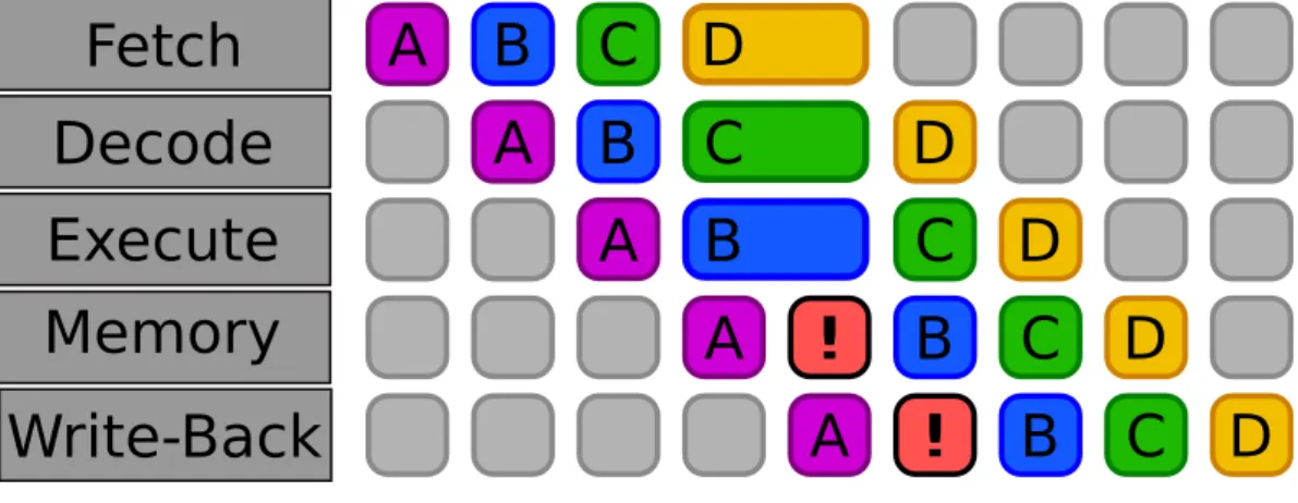
To illustrate pipelining, we present the classic five-stage RISC pipeline displayed in Figure 2.1.5. First we need to look at the RISC instruction set. The basic operations are: ALU instructions, Load and Store, Branch and Jumps. Each instruction in this RISC instruction set can be implemented in at most 5 clock cycles. The 5 clock cycles presented in Figure 2.1.5 are as follows: Instruction Fetch, Instruction Decode, EXecution, MEMory access, Write-Back. Note that branch instructions require 2 cycles, store instruction 4, and all other instructions 5. Although each instruction takes 5 clock cycles to complete, the hardware will be executing some part of the different instructions each cycle, resulting in the execution of an instruction per cycle. From the figure, we see at the first time step the instruction A entering the pipeline:

Figure 2.1.5 – Basic RISC five-stage pipeline [5]

A B C

A B

A

A

A

Fetch

Decode

Execute

Write-Back

Memory

D

B

B

B

C

C

C

C

D

D

D

D

Figure 2.1.6 – Basic five-stage pipeline with a bubble starting at the instruction decode phase

A B C D

A B C

D

A B

C D

A ! B C D

A

!

B

C D

Fetch

Decode

Execute

Write-Back

Memory

the instruction is fetched from memory. At the second step, instruction A is decoded while instruction B enters the pipeline and gets fetched. By adding more instructions in the pipeline every time step, we can hope to completely fill the pipeline. Unfortunately, blindly pipelining instructions is not always the best thing to do. Pipelining hazards can happen. Those are data hazards and control hazards. They can sometimes stall the pipeline, these situations are called pipeline ‘bubbles’. To solve these problems other instruction level parallelism mechanisms can be used.

2.1.4.2 Hazards in pipelines

Let us look at some usual hazards in pipeline and ways to solve them.

Data Hazards happen when an instruction in the pipeline is dependent on the result of another instruction in the pipeline. Consider two instructions: an addition followed by a subtraction. We represent this sequence as follows: ADD R1, R2, R3;

SUB R4, R1, R5;

ADD R1, R2, R3; is the addition operation, where the data in register R2 and R3 are summed and the result is stored in R1. In the same way, SUB R4, R1, R5; is the subtraction operation, subtracting the data in register R1 to data in the register R5 and storing the result in R4. The subtraction is using the result of the addition (the R1 register). If we look back at the pipeline from figure 2.1.5we can see that to perform the ID stage, the SUB needs to wait for the WB stage of the ADD operation. This creates a ‘bubble’ in the pipeline i.e., a time loss for all instructions. Figure 2.1.6shows the creation of a bubble at the ‘decode’ phase. This simple stall can be avoided by using a hardware technique called forwarding (also called bypassing). Indeed, the result of the ADD operation is not really needed until it is actually produced. It can be directly used for the next instruction (the SUB ) without going through the MEM and WB phases. Thus, in the end of the EX phase, a copy of the result is made and fed to the ALU for the next instruction in case of a dependence between two instructions. Note that the MEM and WB phase are still completed after the EX phase as usual.

Unfortunately, bypassing cannot solve all the data hazards. Consider the following sequence:

LD R1, R2; ADD R3, R1, R4;

The LD instruction loads data from memory to processor registers. This in-struction cannot forward the data until the MEM phase. Thus, it would be too late to avoid a stall. A solution to this problem would be to insert another independent instruction between the Load and the Add, thus filling the pipeline. Of course this instruction should not create a stall for it to be a good candidate. This technique is called out-of-order execution or dynamic scheduling. It avoids delays that occur when the data needed to perform an operation are unavailable.

Control Hazards , also called branching hazards, occur when a branch can be taken in a program, for example after an ‘if’ statement. When there are two possibilities, the processor will not know the outcome of the branch before it is computed, and thus will not be able to insert new instructions in the pipeline. There are many methods for dealing with pipeline stalls caused by branch delays. There are for example multiple prediction schemes [9] which look at the most likely way the branch should go and fill the pipeline with these instructions. For example, in a while loop, a scheme could say ‘always assume the while will continue for another iteration’. This will, most of the time, work better than a random scheme as we can assume that if the programmer used a ‘while’ loop, the following instructions should (hopefully for the pipeline) be

performed more than one time.

A ‘recent’ technologies called SMT can also help reduce hazards in pipelines. It was first researched by IBM in 1968. However, the first commercial modern desktop processor to implement SMT was the Intel Pentium 4 released in 2002. It is now included in most of the Intel processor line. This technology is better known under its Intel denomination of ‘Hyperthreading’. Other constructors will follow with sometimes new denomination. IBM releases the POWER5 in 2004 which includes a two-thread SMT engine, Sun Microsystems release the UltraSPARC T1 ‘Rock’ in late 2005 which uses its own ‘CMT’ approach, and so on. The principle is simple: a hyperthreaded core will be executing two (or more) material threads at the same time. However, these threads will be sharing the core’s ALU components. On the physical core, only data and control registers are duplicated. Thus, two hyperthreads also share caches and pipeline. In the end, hyperthreads are helping ILP by filling pipeline hazards. However, two hyperthreads does not mean twice the performances as ALU is not duplicated. At the Pentium 4 release, Intel claimed that the hyperthreaded version added up to a 30% speed improvement.

2.1.4.3 Conclusion on Instruction Level Parallelism

At the beginning of the third millennium, research showed that Instruction-Level Parallelism was at its limit. Indeed, processor were beginning to get

inefficient in terms of performance per watt. Moreover, the complexity of the processors was getting to high, increasing the issue rate. By 2005 the focus shifted to multicore processors. Thread level parallelism would increase performance, and Instruction Level Parallelism would not be the main focus any more. During the same period, SIMD and data-level parallelism saw developments. The next sections introduce Thread-level parallelism as well as Data-level parallelism.

2.1.5

Thread level parallelism

To exploit thread-level parallelism, the MIMD model is often used. It is the architecture of choice for general-purpose (multi-)processors. Indeed, MIMD offers flexibility as it can be used for a single core processor, an application using multiple threads running on a multicore processor as well as for multiple tasks from multiple applications running at the same time. Moreover, MIMD multi-processors can be build efficiently by replicating single processors.

2.1.5.1 Multicore Architectures

As we’ve seen, the improvement of computer performances happened through shrinking integrated circuits. Starting in the 1990s, technology allowed processor designers to place multiple microprocessors on a chip. Each processor is then called a core. Initially called on-chip multiprocessor or single-chip multiprocessor, processor including multiple ‘cores’ are now called multicore. Today they are used in almost all personal computers as well as HPC clusters and in other application domains like embedded, network and so on.

As the clock rate limit was getting closer, increased use of parallelism and thus multicore has been the main research interest to improve overall processing performances. Cores on these processors usually share some resources like second- or third-level caches, or I/O buses for example. These processors are built to exploit the MIMD class of computer parallelism. Each core is executing its own instruction stream. These could be used in general purpose computer to run multiple applications at the same time with more fluidity than with only one core scheduling multiple applications. They can also be used to run multiple threads of the same program as we will see later. Actually, multicore can also be used to exploit data-level parallelism. However, they would cer-tainly be slower than dedicated SIMD machine optimized for these operations. As we will see in a future section, SIMD exploitation requires some prerequi-sites to be optimal. However, taking advantage of a multicore with n cores is usually done with n threads executing the same instructions at the same time. Possible gains are limited by the parallelism that a software can generate

as described by Amdahl’s law presented at the AFIPS Spring Joint Computer Conference in 1967 [10]. These performance gains are called speedup. Amdahl’s law gives the theoretical speedup of a fixed workload that can be expected when system’s resources are improved. It is often used in parallel computing to predict speedup when using more compute nodes or cores for an application, and to determine efficiency of adding more compute resources. Here is the theoretical speedup formula:

1/(1-p)

where p is the part of the workload that can be parallelised. Basically a workload’s speedup is limited by its non-parallel part. By adding an infinite number of resources to a perfectly parallel workload we could reach almost instant computation. However, if the non parallelised part is one hour long, then the resulting execution will be one hour long. Figure 2.1.7 shows the evolution of the theoretical speedup in function of the number of processors. Using the efficiency formula: E = S/p where E is efficiency, S is the speedup gained by a hardware upgrade, and p the parallelism of the target workload, we can determine if making a hardware upgrade is efficient enough or not. For example, it is possible to study the efficiency of making an upgrade compared to its cost.

However, the number of cores is not the only factor to take into account. The raw material for a processor to work is data. This data is stored in memory and needs to find its way to the processor’s registers.

2.1.5.2 Memory Hierarchy

Data are stored in memory. Obviously the best possible memory would be unlimited and fast. The first factor’s limitation is obvious: memory takes space on chips, thus it is not possible to fit unlimited memory there. It is possible to get a very large amount of memory a little further away from the processor, but then we affect the second factor as we get higher latency than close on-chip memory. A clever solution to these two factors is memory hierarchy.

The locality of reference or principle of locality tells us that an application as the tendency to access the same set of memory locations repetitively over a short period of time. This is due to the way codes are written, using loops and arrays and updating the same set of data over and over. In fact, widely held rule of thumb is that a program spends 90% of its time in 10% of the code. This 10% are loops, accessing the same data multiple time or contiguous data objects that can be fetched by batch. Then we can differentiate between two types of reference locality. Temporal locality, the first one, refers to the use of the same data within a small duration time. The second, spacial locality,

refers to the use of data elements close to one another. There is also a special case of spacial locality called sequential locality where arranged data elements are accessed linearly, such as going through an array. This principle of locality (as well as the cost of large and fast memory) led to hierarchies of memory of

different sizes and speeds.

Memory is organized into a hierarchy of several levels where each level is smaller, faster, and more costly per bit than the previous one. The objective is to provide a memory system with speed almost as fast as the last level, but with cost and size of the first. Here are the main levels present in almost every memory hierarchy.

• Registers: The smallest memory on the processor. Registers may hold an instruction, a storage address, or any kind of data. Usually one word or a couple words of data in vectorial processors. The processor units (the ALU) directly use data contained in registers to perform computations. This is the fastest memory, directly accessed by the processor, present in very limited amount.

• Caches: This memory is really close to the cores. It is actually embedded in microprocessors and thus is extremely quick to access. However, as space is limited on the chip, cache memory is really small. They range from tens of KB to a hundred MB of data.

• Main memory: Main memory provides data to caches and serves as I/O interface. It is also called RAM (Random Access Memory). Modern compute node typically have around 256 GB of memory per node. • Disks: really large storage devices. They are used to store the machine’s

file system. Depending on usage, these disks can be as fast as SSD and as slow as LTO (Linear Tape-Open). As multiple disk can be used, capacity is almost unlimited.

Most CPUs have multiple caches. First, a hierarchy of instruction caches. These caches contain the instructions to be executed by the processor. Then a second hierarchy, this time containing data. We often talk of cache levels (L1, L2, L3 and so on). Usually with multicore processors, each core has access to its own L1 and L2 caches. The first level is often split for instruction (L1i) and data (L1d). The L2 cache is only used for data. Then the L3 cache is shared between all cores. L4 and higher cache level are highly uncommon. Usually, L1 cache is only a couple dozen of KB per core. L2 is a bit larger with a few hundreds KB per core. L3 would be between a hundred MB and a GB per chip. As caches are tiny, programs are loaded into main memory to be executed. Main memory is significantly larger than caches with up to hundreds of GB (and reaching the TB). However, it is also significantly slower. The order of magnitude to read data is 1 cycle to read a register, less than 5 to read in L1 cache, 10 to 15 to read in L2 and less than 100 to read in L3. Reading data from main memory is around 200 to 400 cycles. Lastly, at the

Figure 2.1.8 – Diagram of a basic four node NUMA system

C1

C2

C3

C4

C1

C2

C3

C4

C1

C2

C3

C4

C1

C2

C3

C4

end of the hierarchy we can find disks. These are really slow, even compared to RAM memory. Access to data in disks could cost a dozen ms (where RAM access is around 100ns and L1 cache less than 1ns). However, they are really cheap compared to the other memories and thus offer almost unlimited storage. Actually, tape data storage is used to store large amounts of data that don’t need to be read often. This technology is useful for its cheap price, and low power consumption as tapes don’t need to be powered. Accessing data stored on disks takes a few seconds to minutes depending on the technology used.

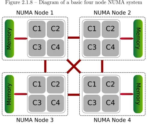
2.1.5.3 Non Uniform Memory Access (NUMA)

An additional factor to take into account when looking at memory access time is distance from each core to the memory. Indeed, two memories from the same hierarchy level can have different access times. This is the case on NUMA systems which are often used in HPC clusters. Under the NUMA memory design, a processor can access its own local memory faster than non-local memory. The non-local memory could be memory local to another processor or memory shared between processors. Figure 2.1.8 is the representation of a simple 4 processors NUMA node. Multiple cost-effective nodes on different sockets are connected by a high-performance connection. Each node contains processors and memory. However, a node is allowed to use memory from all other nodes thanks to a memory controller that keeps memory coherency. Access time to remote memory will obviously be slower than local memory. This

is called the NUMA effect. This means that using memory efficiently takes some thinking but the upside is in limiting the number of message exchange. Indeed, NUMA effect between two cores on the same NUMA system will certainly be less time-consuming than the cost of messages sent on the network.

2.1.6

Data level parallelism in vector and manycores

There are two main variations around SIMD: vector architectures (actually designed in the 70s), and graphics processing units (GPUs). As SIMD will not be a focal point of this thesis, this section only highlights the main principles of these SIMD variations.

2.1.6.1 Vector Architecture

Vector processors (also called array processors) are designed to operate on multiple data at the time. Vectors are one-dimensional arrays of data. With a single instruction, the processor will operate on all the data contained in the vector. Data are then put back into memory. The issue is to get data from memory to the processor. Indeed, filling the vector requires a large amount of data. To reduce the time consumed by load and stores, these steps are deeply pipelined. In the end, working on a lot of data at the same time with one instruction (i.e., using large vectors) helps hiding the memory latency. However, large vector means specific set of data, with no data dependencies or hazards. This also means that when parallelism is not optimized for vectors (i.e., when using instruction on small vectors), this kind of processors becomes

less efficient.

2.1.6.2 Manycore architectures

Manycore processors are architectures using a lot more cores than traditional multicore processors. They are composed of simpler cores, worst at single thread performances but optimized for higher throughput and/or lower consumption. They benefit from high degrees of parallelism. In fact, using these architectures for MIMD would be highly inefficient. Moreover, to limit energy consumption and provide more space for cores, these chips usually do not include out-of-order execution technology, deep pipelines, and large caches. There exists many specific manycore architectures. During this thesis, I used the Intel Xeon Phi, which has MIC (Many Integrated Cores) architecture. The first commercialized in 2013, called Intel Knights Corner (KNC), was a coprocessor using 57 to 61 cores. Each core was using 4 hyperthreads. The version I used during this PhD is the Intel Knights Landing (KNL), commercialized in 2016. This one is composed of 64 to 72 cores, with still 4 hyperthreads per core. On the other hand, another kind of manycore are GPUs (Graphic Processing Unit). These can be described as manycore vector processors. Originally designed to

rapidly manipulate and alter memory to create images intended for output to a display, they have been redesigned to be used in HPC clusters. Thus, all the cores can only execute simple instructions. Moreover, at each clock tick, every core is executing the same instruction (on different data). This highly parallel structure makes them really efficient for algorithms that process large block of data in parallel. In HPC, this is particularly interesting for matrix computations used in simulations.

2.1.7

Conclusion on evolutions

Evolutions presented are not the only ones that permitted computer perfor-mance growth rate. Other evolutions in memory, cache, software also helped. These evolutions are not presented here as they don’t add that much to the point we are trying to make: architectures are becoming complex, with a lot of processors, cores, hardware threads, deep memory hierarchies and so on. This complexity brought better possible performances, but also more complex programs and optimizations. The next sections present the actual look of HPC clusters architecture as well as techniques used to harness their compute power.

2.2

Supercomputer Architecture

Simulations are often iterative calculations, each step refining the solution. The closer the computed solution is to the measured value, the more accurate the solution is. The objectives of current supercomputer is to compute fast and accurate simulations. The next global goal is to reach the Exascale milestone. To do so, they use all the resources at their disposal. As we have seen, architectures are always evolving and supercomputers use the best innovations among them. Today in HPC, supercomputers are massively parallel systems. Figure2.2.1 shows how supercomputers can be assembled. They are composed of a large quantity of nodes linked together. A node is itself composed of multiple multicore processors, and sometimes also connected to accelerators like GPUs. Each node uses its own operating system. In the end, programming applications for these architectures is a complex task. Programmers need to create highly parallel code taking clusters’ topology into account. This means code capable of using a large quantity of nodes and cores, accessing memory efficiently, not wasting time in communication and so on. Moreover, each generation of supercomputer adds a layer of complexity and the exascale machine will, without a doubt, provide even larger problems to the code developers [12].

Figure 2.2.1 – Architecture of the Blue Gene/L Supercomputer [11]

2.2.1

Supercomputers Tops

Before we can look at how to use these complex architecture, let us look at the current most powerful computer systems in the world. A couple of tops exist to determine which computer is the ‘best’. In HPC the Top500 [13] is the most used one. Twice a year, machines are compared on a specific benchmark and the best 500 are ranked. This benchmark is the Linpack benchmark [14]. It computes the solution of a dense linear system with n equations and n unknown. In the end, it determines the Flops of the computer (i.e., the number of floating-point operation it can compute per second).

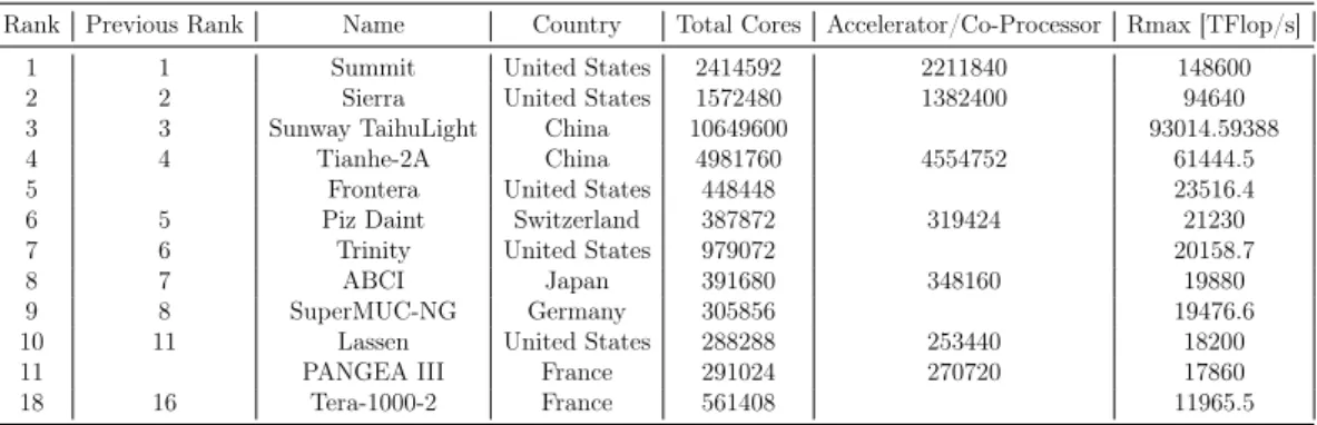
Table 2.2.1 shows the last Top500 highest ranked computers (results from the June 2019 Top500 ranking). We can see that the United States dominates the ranking with the top two places, as well as 5 computers in the top 10. China is not far behind with two computers at the third and fourth places. France’s first computer to appear in the Top500 is PANGEA III, an industrial machine from the Total firm. It is also the most powerful industrial computer of the Top500. The first research computer from France, Tera-1000-2 from the CEA places as sixteenth. However, the Flops metric does not entirely reflect HPC applications. While it is true that some codes do a lot of matrix computations that are highly parallel, some don’t.

Rank Previous Rank Name Country Total Cores Accelerator/Co-Processor Rmax [TFlop/s] 1 1 Summit United States 2414592 2211840 148600 2 2 Sierra United States 1572480 1382400 94640 3 3 Sunway TaihuLight China 10649600 93014.59388 4 4 Tianhe-2A China 4981760 4554752 61444.5 5 Frontera United States 448448 23516.4 6 5 Piz Daint Switzerland 387872 319424 21230 7 6 Trinity United States 979072 20158.7

8 7 ABCI Japan 391680 348160 19880

9 8 SuperMUC-NG Germany 305856 19476.6 10 11 Lassen United States 288288 253440 18200 11 PANGEA III France 291024 270720 17860 18 16 Tera-1000-2 France 561408 11965.5

Table 2.2.1 – Top 10 best ranked computer in the Top500 plus the fist two French ones

Thus, other benchmarks and tests are proposed. In particular, the High Performance Conjugate Gradient (HPCG) benchmark, which uses the Conju-gate Gradient algorithm, is intended to complement the Linpack benchmark. Table 2.2.2 shows the top computers ranked with this benchmark (results from June 2019). The United States are also well represented in this top with the top two places and 4 computers in the top 10. We can also see that Summit and Sierra are the top two computers of the two rankings. The third computer in this top is the K computer from Japan which was 20th in the Top500. This shows that the two rankings and benchmarks look at different optimizations made in computers architectures. Tera-1000-2, the French su-percomputer from CEA, is just outside the top 10 with the 11th place. But performance is not the only issue any more, energy consumption is also a limit-ing factor for supercomputers. It is now at the core of architectures innovations.

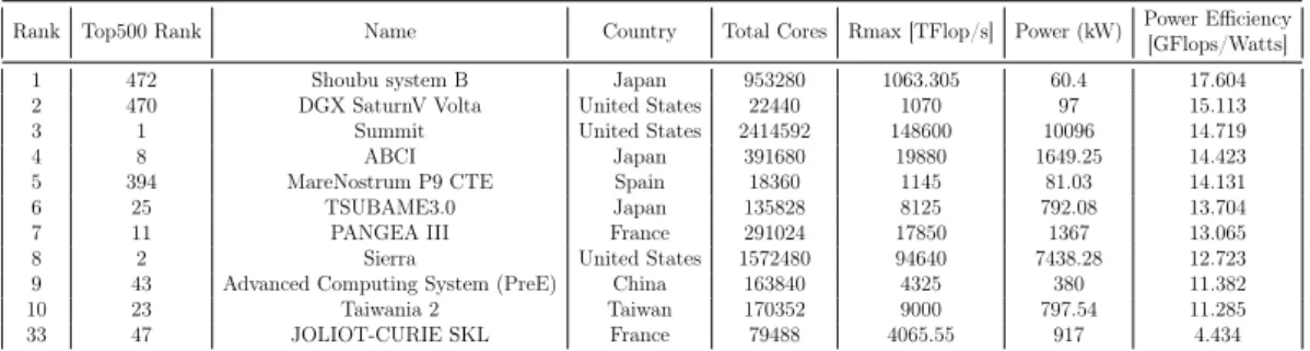
To reflect this focus, another ranking can be used. It is called the Green500, and ranks computers from the Top500 depending on their energy consumption (or GFlops/watt). Table2.2.3 shows the results of the last Green500 ranking (results from June 2019). This time Japan and the United States are dominating the top 10 with 3 computers each and the four top places. We can see that a couple of top 10 computers from the Top500 are still well places here. Summit and Sierra, the first two computers of the Top500 (and HPCG) from the United States as well as ABCI the 7th from Japan. The fact that Sierra and Summit appear in the top 10 of these three rankings shows that the new supercomputers look for low energy consumption to reach higher performances.

2.3

Parallel programming models

We have seen that HPC architectures are becoming more and more complex. To exhibit more parallelism, more cores are added, but memory per core is

Rank Top500 Rank Name Country HPCG [PFlop/s]

1 1 Summit United States 2.926

2 2 Sierra United States 1.796

3 20 K computer Japan 0.603

4 7 Trinity United States 0.546

5 8 ABCI Japan 0.509

6 6 Piz Daint Switzerland 0.497

7 3 Sunway TaihuLight China 0.481

8 15 Nurion Korea 0.391

9 16 Oakforest-PACS Japan 0.385

10 14 Cori United States 0.355

11 18 Tera-1000-2 France 0.334

Table 2.2.2 – Top 10 best ranked computer with HPCG Benchmark plus the first French one

Rank Top500 Rank Name Country Total Cores Rmax [TFlop/s] Power (kW) Power Efficiency

[GFlops/Watts]

1 472 Shoubu system B Japan 953280 1063.305 60.4 17.604

2 470 DGX SaturnV Volta United States 22440 1070 97 15.113

3 1 Summit United States 2414592 148600 10096 14.719

4 8 ABCI Japan 391680 19880 1649.25 14.423

5 394 MareNostrum P9 CTE Spain 18360 1145 81.03 14.131

6 25 TSUBAME3.0 Japan 135828 8125 792.08 13.704

7 11 PANGEA III France 291024 17850 1367 13.065

8 2 Sierra United States 1572480 94640 7438.28 12.723

9 43 Advanced Computing System (PreE) China 163840 4325 380 11.382

10 23 Taiwania 2 Taiwan 170352 9000 797.54 11.285

33 47 JOLIOT-CURIE SKL France 79488 4065.55 917 4.434

Table 2.2.3 – Top 10 best ranked computer in the Green500 plus CEA’s best one

getting smaller. To limit energy consumption, co-processors are added to the already complex multiprocessors nodes. In the end, machines are made of nodes with dedicated memories linked together by a network. Each node is then composed of multicore processors with their own memory but also sharing collective memory with each other. Co-processor and accelerators like GPUs can also be added to the mix. To exploit all these resources, application developers need to create highly parallel codes, by taking complex architectures into account. To minimize the complexity of programming on these clusters, programming models have emerged. They are an abstraction of the parallel computer architecture used to express parallel algorithms. They are evaluated on there generality (how many problems they can express and how many architectures can use them), and performances. This section presents the main ones and their basic mechanisms. Programming models are separated into two big groups: shared-memory models to help manage memory shared by multiple cores of the same node, and distributed memory models that are used to send messages between cores or nodes all over the machine.

2.3.1

Shared-memory models

Processors are now composed of multiple cores. All the cores of a processor have access to its memory. Moreover, cluster nodes are often composed of multiple processors creating NUMA nodes. These nodes also have memory shared by all the processors. Using a shared memory programming model on these kinds of architectures allows multiple threads or processes running on the same processor or node to share data and communicate. Threads read and write asynchronously in shared memory. Asynchronous access to memory can lead to race conditions when multiple threads read and write in the same location. Specific techniques are used to avoid these hazardous behaviours. Programmers can implement locks, mutex, semaphores and in a larger extent critical sections to protect data from race conditions. All these mechanisms can be used to ‘protect’ variable from concurrent accesses and thus certify memory coherence. If a multi-threaded code only manipulates shared data structures so that all threads can’t have unintended interactions it is said thread safe. We then present the two most commonly used shared programming models in HPC, POSIX threads and OpenMP.

2.3.1.1 POSIX Threads

POSIX Threads, usually referenced to as pthreads, is part of the POSIX (Portable Operating System Interface) standard. This standard specified by the IEEE Computer Society is used to maintain compatibility between operating systems. The POSIX Thread part defines an API to create, control multiple flows of work that overlap in time. These flows are called threads. To understand