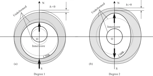
Degree one loading by pressure variations at the CMB
15
0
0
Texte intégral
Figure


Documents relatifs