HAL Id: hal-01806181
https://hal.archives-ouvertes.fr/hal-01806181
Submitted on 28 Oct 2020
HAL is a multi-disciplinary open access
archive for the deposit and dissemination of
sci-entific research documents, whether they are
pub-lished or not. The documents may come from
teaching and research institutions in France or
abroad, or from public or private research centers.
L’archive ouverte pluridisciplinaire HAL, est
destinée au dépôt et à la diffusion de documents
scientifiques de niveau recherche, publiés ou non,
émanant des établissements d’enseignement et de
recherche français ou étrangers, des laboratoires
publics ou privés.
Alina Găinuşă-Bogdan, Pascale Braconnot, Jérôme Servonnat
To cite this version:
Alina Găinuşă-Bogdan, Pascale Braconnot, Jérôme Servonnat. Using an ensemble data set of turbulent
air-sea fluxes to evaluate the IPSL climate model in tropical regions. Journal of Geophysical Research:
Atmospheres, American Geophysical Union, 2015, 120 (10), pp.4483 - 4505. �10.1002/2014JD022985�.
�hal-01806181�
RESEARCH ARTICLE
10.1002/2014JD022985
Key Points:
• Database of 14 turbulent air-sea flux products is assembled for model evaluation
• Proposed methodology is suited for systematic large-scale model evaluation
• Robust biases in state variables do not result in robust biases in IPSL fluxes
Correspondence to:
A. G˘ainu¸s˘a-Bogdan,
alina.gainusa-bogdan@lsce.ipsl.fr
Citation:
G˘ainu¸s˘a-Bogdan, A., P. Braconnot, and J. Servonnat (2015), Using an ensemble data set of turbulent air-sea fluxes to evaluate the IPSL climate model in tropical regions, J. Geo-phys. Res. Atmos., 120, 4483–4505, doi:10.1002/2014JD022985.
Received 16 DEC 2014 Accepted 1 APR 2015
Accepted article online 15 APR 2015 Published online 19 MAY 2015
©2015. American Geophysical Union. All Rights Reserved.
Using an ensemble data set of turbulent air-sea fluxes to
evaluate the IPSL climate model in tropical regions
Alina G ˘ainus¸ ˘a-Bogdan1,2, Pascale Braconnot1, and Jérôme Servonnat1
1Laboratoire des Sciences du Climat et de l’Environnement, Unité mixte CEA-CNRS-UVSQ, Gif-sur-Yvette Cedex, France, 2Laboratoire de Météorologie Dynamique, Intitut Pierre Simon Laplace, Paris, France
Abstract
Ocean-atmosphere interactions represent a key component of the hydrological cycle in tropical regions and their variability has profound influences on low-latitude climate. In order to evaluate how climate models represent these fluxes while taking into account the observational uncertainties, we assemble a comprehensive database of 14 climatological surface flux products, including in situ-based, satellite, hybrid, and reanalysis data sets. We find that the large observational uncertainties are reflected in the climatological magnitudes, as well as in the spatial patterns and seasonal variations and that, for the most part, they do not carry specific signatures of product type. This data ensemble allows us to draw several conclusions on the current representation of the intertropical turbulent air-sea fluxes in the atmospheric component of the Intitut Pierre Simon Laplace-Coupled Model 5A, when forced by observed sea surface temperatures. Despite significantly underestimated near-surface wind speeds over the entire tropical oceans domain, the atmospheric model produces generally well represented zonal and meridional wind stress values, and only weak biases in the spatial patterns and seasonality. The simulated latent heat flux develops a bias pattern matching that of the wind speed, but with no systematic underestimation. Compared to the same reference, the sensible heat flux is overestimated over the entire region of interest, in response to a significant overestimation of the sea-air temperature contrast. The observational ensemble and analyses presented in this paper offer a good framework for large-scale model surface flux evaluation.1. Introduction
Ocean-atmosphere heat and water fluxes play a major role in the global climate, as they determine the vertical transport of heat, momentum, and moisture and their availability for meridional transport and exchange with the other components of the climate system.
These fluxes are expected to be modified in response to climate change, introducing a complex feedback in the evolution of the global climate. However, the nature of this response is yet uncertain. Furthermore, due to their coupling role on smaller time scales, they also have an important effect on seasonal and decadal model prediction skill [Gulev et al., 2008]. Their correct representation in global numerical models is thus of chief importance [Barnier, 2001], as is the development of quantitative and objective methods of evaluation of simulated fluxes with observations.
In this paper we are interested in evaluating the representation of the turbulent ocean-atmosphere interactions in the Intitut Pierre Simon Laplace-Coupled Model 5A (IPSL-CM5A) at low latitudes. The choice of this region is motivated by the ongoing improvement on tropical convection in the IPSL model [Rio et al., 2013]. A future revision to the model will concern the representation of the turbulent surface fluxes. This is why they represent the focus of the present evaluation, the radiative fluxes being beyond the scope of this study. The IPSL-CM5A model is part of the Coupled Model Intercomparison Project Phase 5 (CMIP5) modeling exercise and is presented in detail by Dufresne et al. [2013]. In this study we present the first step of this assess-ment, focused on its atmospheric component, LMDZ5A. This evaluation considers not only the flux estimates but also the available meteorological variables used in the flux calculations.
In models as well as global gridded observational products turbulent fluxes are based on bulk formulae. Surface wind stress (𝜏), latent heat flux (LH) and sensible heat flux (SH) are thus estimated as follows:
LH = Λ𝜈𝜌CE(q(z) − qsat(𝜃0))|Δ⃗U(z)| (2)
SH =𝜌cpCH(𝜃(z) − 𝜃0)|Δ⃗U(z)| (3)
where𝜌 is the near-surface air density, Δ⃗U is the relative surface wind (sometimes approximated to the near-surface wind velocity, the ocean surface current being neglected), q is the near-surface specific air humidity, qsatis the saturation humidity at the sea surface temperature,𝜃0and𝜃 are the surface and the
near-surface potential air temperatures, respectively, Λ𝜈is the latent heat of vaporization and cpthe specific
heat of air. The wind speed, air temperature, and air humidity are attributed to a standard level z, usually 10 m above the surface. The bulk transfer coefficients for momentum (CD), humidity (CE), and sensible heat (CH) are parameterized as functions of wind speed and atmospheric stability, as well as, in some cases, other factors (e.g., sea state) [Jones and Toba, 2001]. These parameterizations vary considerably from one study to another [Dyer, 1974; Blanc, 1985; Fairall et al., 2010], potentially representing the main source of uncertainty in the flux estimates in many cases, especially for LH [Brunke et al., 2011].
Evaluating a model naturally implies having a reference against which to compare the model. Several types of flux products are now available. They have been developed from in situ measurements [da Silva et al., 1994;
Berry and Kent, 2009; Hughes et al., 2012], satellite observations [Andersson et al., 2010; Tomita et al., 2010; Bentamy et al., 2003; Shie et al., 2010], or meteorological reanalyses [Kalnay et al., 1996; Onogi et al., 2007; Dee et al., 2011]. Hybrid products also consider reanalyses together with other types of observations [Yu and Weller, 2007; Kumar et al., 2012; Large and Yeager, 2009; Brodeau et al., 2010]. Uncertainties in the different
types of retrieval of the meteorological state variables, in the parameterization of the transfer coefficients and differences in the assembly of the final-gridded products all add to the uncertainty of surface flux products. The large uncertainties in the “observational” turbulent flux fields have been widely discussed in the literature and shown to be on the order of 0.01–0.02 N m−2for wind stress, 30–60 W m−2for the latent heat flux, and
10–15 W m−2for the sensible heat flux, or up to 0.04 N m−2for wind stress and up to 100 W m−2for the
sur-face heat flux [Kumar et al., 2012; Tomita et al., 2010; World Climate Research Programme (WCRP), 2000; Bourassa
et al., 2008; Smith et al., 2011; Chaudhuri et al., 2013; Josey and Berry, 2010; Gulev et al., 2010; Röske, 2006].
They need to be accounted for in model evaluation [Braconnot and Frankignoul, 1993] and are a reason why estimating the quality of simulated fluxes and of their feedbacks requires the development of specific strategies. Yet, due to the difficulty in estimating it, observational uncertainty is rarely explicitly included in analyses of model results, as done by Wittenberg et al. [2006] for the tropical Pacific. The most recent large-scale model flux evaluation study of Bates et al. [2012] employs a single-observational reference for most of its analyses. It is only for an assessment of regional averages that this is put in the context of the multiproduct analysis of Röske [2006]. In their key paper on climate model performance, Gleckler et al. [2008] take into account the observational uncertainty by calculating the large-scale metrics against two reference products. While for particular regions, time periods, or applications some flux products are shown to be superior to others or certain products are shown to be unsuitable [World Climate Research Programme (WCRP), 2000; Smith
et al., 2011; Tomita et al., 2010; Yu et al., 2011; Kumar et al., 2012; Röske, 2006], there is currently no consensus on
one global data set to be used for large-scale model surface flux validation [World Climate Research Programme
(WCRP), 2000; Bourassa et al., 2008; Smith et al., 2011; Gulev et al., 2010; World Climate Research Programme (WCRP), 2012]. Therefore, our approach is to consider the major available climatological gridded surface flux
products that we combine into an observational ensemble to compare our model results with.
In a first step, we describe the observational database. We characterize the spread between the different flux products and related atmospheric and oceanic variables, we check the consistency between the products and investigate whether there are systematic biases pertaining to the different product types. The results of this first analysis consolidate the observational ensemble approach for our purposes. We then use this data compilation to evaluate the representation of intertropical ocean-atmosphere turbulent fluxes in the IPSL-CM5A model [Dufresne et al., 2013], starting with its atmospheric component LMDZ5A [Hourdin et al., 2013]. Rather than attempting to calculate a skill score for the model, our focus is on the identification of the robust flux-related biases in the model climatology. Wherever the model results fall outside the so-defined observational envelope, a significant model bias is identified and can be targeted for model improvement
Table 1. Summary of Observational Data Sets Used in This Studya
Data Category Data Set Period Covered Reference
In situ- Da Silva 1945–1989 da Silva et al. [1994]
based NOC2 (Version 2 of the National 1973–2011 Berry and Kent [2009]
Oceanography Center flux data set)
FSU3 (Florida State University fluxes) 1978–2004 Hughes et al. [2012]
Satellite- HOAPS3 (Version 3 of the Hamburg 1988–2005 Andersson et al. [2010]
based Ocean Atmosphere Parameters and
Fluxes from Satellite data)
J-OFURO2 (Japanese Ocean Flux 1988–2007 Tomita et al. [2010]
Data Sets with Use of Remote Sensing Observations)
IFREMER 1993–2007 Bentamy et al. [2003]
GSSTF2b (Version 2 of the Goddard 1988–2008 Shie et al. [2010]
Satellite-Based Surface Turbulent Fluxes)
Reanalysis NCEP/NCAR (National Centers for 1948 to the present Kalnay et al. [1996]
Environmental Prediction/ National Center for Atmospheric Research reanalysis)
JRA25 (Japanese 25 year reanalysis) 1979–2005 Onogi et al. [2007]
ERA-Interim (European Center for 1979 to the present Dee et al. [2011]
Medium-Range Weather Forecasts reanalysis)
Hybrid OAFlux (Objectively Analyzed air-sea 1958–2009 Yu and Weller [2007]
Fluxes for the Global Oceans)
TropFlux 1989–2011 Kumar et al. [2012]
CORE2 (GFDL version 2 forcing for 1949–2006 Large and Yeager [2009]
common ocean-ice reference experiments)
DFS4 (DRAKKAR Forcing Set v4.3) 1958–2006 Brodeau et al. [2010]
aThe underlined characters represent the short names for the observational data sets. These are the names
used throughout the document to refer to observational products. What follows these short names in the table, in parentheses, are, where applicable, the corresponding extended names.
and accounted for in studies using that model. We mainly focus on aspects that can be of interest for the evaluation of other models, such as climatological magnitudes and spatial patterns, shape and amplitude of the seasonal cycle, and coherence with large-scale atmosphere and ocean dynamics.
The manuscript is organized as follows: the observational and model data used in the analysis, as well as the preliminary data treatment, are presented in section 2. In section 3 we first offer a brief overview of the main statistics employed in the analyses. We then describe the observed distribution of turbulent air-sea fluxes in the intertropical region, quantify the observational uncertainty of the fluxes and of the associated surface state variables and address the question of systematic differences between different observational data types. Section 4 presents the LMDZ5A model results in comparison with the observational ensemble, all the while considering the intervariable relationships. We conclude the paper with a discussion and summary of our findings in section 5.
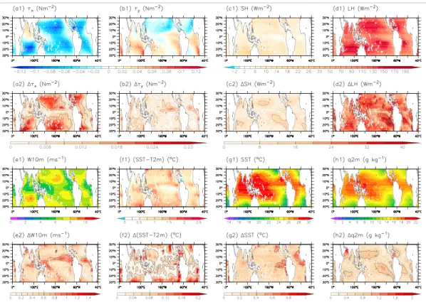
Figure 1. Average observed climatological annual mean (a1) zonal wind stress, (b1) meridional wind stress, (c1) sensible
heat flux, (d1) latent heat flux, (e1) near-surface wind speed, (f1) sea-air temperature contrast, (g1) sea surface temperature, (h1) near-surface specific air humidity over the intertropical oceans. (a2–h2) The corresponding obser-vational uncertainty, calculated as either the maximum observed departure of a data set from the ensemble mean (equation (4), colors) or the root-mean-square pairwise distance between the observational products (equation (6), contours). The contours coincide with consecutive interval limits on the corresponding color bars, except for (e2), where
the contour spacing corresponds to 0.2 m s−1and (f2), where it corresponds to 0.08◦C; in each subfigure, the level of a
sample, dark contour, is indicated by a similar tick mark on the color bar. Note that the reanalyses are not considered in the observational ensemble.
2. Data Sets: Observations and Simulations
2.1. Observational-Based Products
In an intercomparison of observational flux products, Smith et al. [2011] have shown that different obser-vational strategies are in order depending on the study aims. To our current knowledge, there is no one ideal climatological data set to be used for general, large-scale validation of the representation of turbulent surface fluxes in climate models. We thus assemble a comprehensive observational database, covering differ-ent types of turbuldiffer-ent flux products, which we use to establish a range of reasonable climatological values, spatial patterns, and seasonal variations to compare our model results with (Table 1).
We restrict the database to available gridded data sets over the intertropical oceans for the latent heat flux (LH), the sensible heat flux (SH), the zonal wind stress (𝜏x), the meridional wind stress (𝜏y), and the meteorological surface parameters used to calculate these fluxes, namely, the 10 m level wind speed (W10m), the sea-air temperature gradient using the sea surface and 2 m level air temperatures (ΔT2m), the sea surface temperature (SST), and the 2 m level specific air humidity (q2m) (Figure 1). The availability of these variables for each data set (Table 1) is given in Table 2. Note that different products offer the air temperature and humidity at two different standard levels, 2 m and 10 m above the surface, 10 m being the standard altitude generally used in the bulk formulae flux computations. Here we have chosen only the 2 m level temperature and humidity, as they directly correspond to the output of the model to be evaluated.
Our observational database includes three in situ-based data sets (Table 1). In situ measurements (from research or voluntary observing vessels, buoys, and floats) cover longer time periods and include research quality climatological data, but the corresponding global gridded data sets often suffer from poor and inhomogeneous sampling and inherent observational biases and uncertainties, including problems of
Table 2. List of Data Sets and Variables Analyzed in This Studya Variables Data Set LH SH 𝜏x 𝜏y W10m T2m SST q2m AMIP ✓ ✓ ✓ ✓ ✓ ✓ ✓ ✓ Da Silva ✓ ✓ ✓ ✓ - - ✓ -NOC2 ✓ ✓ - - ✓ - ✓ -FSU3 ✓ ✓ ✓ ✓ ✓ - ✓ -HOAPS3 ✓ ✓ - - ✓ - ✓ ✓ J-OFURO2 ✓ ✓ ✓ ✓ ✓ - - -IREMER ✓ ✓ ✓ ✓ ✓ - ✓ -GSSTF2b ✓ ✓ ✓ ✓ ✓ - - -NCEP/NCAR ✓ ✓ ✓ ✓ ✓ ✓ ✓ ✓ JRA25 ✓ ✓ ✓ ✓ - ✓ ✓ ✓ ERA-Interim - - ✓ ✓ ✓ ✓ ✓ -OAFluxb ✓ ✓ - - - - ✓ -TropFlux ✓ ✓ - - ✓ ✓ ✓ ✓ CORE2 ✓ ✓ ✓ ✓ - - - -DFS4 ✓ ✓ ✓ ✓ ✓ ✓ ✓ ✓
aCheckmark and dash indicate the availability and absence of the
corresponding field, respectively.
bOAFlux now providesW10m,q2m, andT2mdata. However, at the
time the observational data was assembled, technical difficulties con-cerning data access prevented their inclusion in this study.
variable corrections [Josey et al., 1999; Kent and Berry, 2005; Kent et al., 2007; Gulev et al., 2007a, 2007b; Bourassa
et al., 2008; Smith et al., 2011; Brunke et al., 2011]. The older, Da Silva data set, in particular, has been excluded
from some analyses [e.g., Smith et al., 2011], as it has been shown to suffer from many caveats in recent years, including having a limited time overlap with other products (Table 1), sampling problems [Kubota et al., 2002, 2003; Chou et al., 2003] and an underestimation of the oceanic heat loss [Gulev et al., 2010]. However, given the extensive past use of this data set [Jones et al., 1999; World Climate Research Programme (WCRP), 2000;
Moore and Renfrew, 2002; Kubota et al., 2002; Chou et al., 2003; Gleckler, 2005; Wittenberg et al., 2006; Hughes et al., 2012], we include it in our analysis and test whether it stands out as an outlier compared to more
modern products.
The in situ products are complemented, in this study, by four satellite-based observations (Table 1). Satellite measurements provide a good answer to the spatial sampling problem and in some locations to that of temporal sampling, compared to in situ data, and, within each product, they are bound to be more consistent in space and time. However, they have shorter time coverage and their characteristics change with changes in the observing system. They are also subject to a different set of uncertainties linked to the retrieval algorithms for the variables of interest, especially for air temperature and humidity [Bourras, 2006; Bourassa et al., 2008;
Smith et al., 2011; Brunke et al., 2011]. Furthermore, they may contain systematic weather or process-related
(e.g., rain and atmospheric stratification) biases and uncertainties [Smith et al., 2011], severely hindering their use for general studies at climatological scale.
While not a proper observational product type, another category of data extensively used for climate monitoring, climate model evaluation, and climate studies in general is reanalysis data. For each reanalysis product, these data are obtained through the assimilation of all available observations in a model that remains unchanged over time [see National Center for Atmospheric Research, 2013; Reanalyses.org, 2013]. This provides dynamically consistent, three-dimensional, global gridded data sets of a large array of variables, with typically long time coverage. On the other hand, reanalysis data suffer from model-related problems, like the poor representation of the atmospheric boundary layer and of equatorial winds or various problems with parameterizations [Bourassa et al., 2008; Smith et al., 2011; Moore and Renfrew, 2002]. Importantly, the spatial and temporal distribution, and source of the assimilated data are variable, according to the input data availability, which can introduce inhomogeneities in time, even unphysical behaviors [Josey and Berry, 2010;
Smith et al., 2011; Yu et al., 2011] or significantly time-dependent errors [Kubota et al., 2008; Chaudhuri et al.,
2013]. Here we consider three reanalyses, listed in Table 1.
Finally, we added four hybrid flux products (Table 1). Blended or hybrid data sets use various statistical methods to combine data from the categories described above as well as information about the input data errors and proposed corrections, in order to obtain optimized large-scale gridded data sets for specific needs (e.g., global energy balance; forcing of ocean general circulation models—CORE2 and DFS4). By design, this type of product combines some of the strengths, but also some of the weaknesses, of the original fields it is based on [Fairall et al., 2010].
It should be noted that the delimitations between the four flux product categories listed above are not always unequivocal. For example, while constructed mostly from in situ/satellite data, the FSU3, J-OFURO2, and GSSTF2b products each include at least one variable that belongs to a different data type. The SST field used in the FSU3 product is the blended product from the National Meteorological Center [Hughes et al., 2012;
Reynolds, 1988]. J-OFURO2 also uses a blended SST field, the Merged satellite and in situ data Global Daily
Sea Surface Temperatures but also the National Centers for Environmental Prediction (NCEP)/Department of Energy Reanalysis 2 for the near-surface air temperature [Tomita et al., 2010]. The same reanalysis is used for the air temperature, sea skin temperature, and sea level pressure in GSSTF2b [Shie et al., 2010]. These characteristics could qualify them for the hybrid product category. Here, however, we have considered as proper hybrid products only those products using several types of data and either employing specifically designed merging procedures or further ad hoc corrections to the initially obtained fields.
2.2. Atmospheric Model Intercomparison Project Simulations
We consider historical LMDZ5A simulations for the 1979–2010 period with prescribed observational sea surface temperatures and sea ice cover, according to the CMIP5 protocol for Atmospheric Model Intercomparison Project (AMIP) experiments [Taylor et al., 2000; Hurrell et al., 2008].
A complete description of the LMDZ atmospheric model can be found in Hourdin et al. [2006, 2013]. In particular, the atmospheric surface boundary layer is parameterized using the scheme proposed by Louis [1979], based on the Businger-Dyer bulk formula [Businger, 1966, 1988]. At the ocean interface the roughness length is computed following Smith [1988] for momentum and includes the Charnock formulation and a smooth flow term. Since this version of the model uses the same neutral drag coefficient for momentum and heat fluxes, a factor of 0.8, corresponding to a mean ratio between the heat and momentum exchange coefficients [Smith, 1988], is applied to the turbulent heat exchange coefficient to account for a lower drag [Smith, 1988].
The input variables are prognostic variables at the first model level, roughly 35 m above the surface in the tropics. However, these are not directly comparable to available observational meteorological variables. For this purpose we use diagnostic model variables for 10 m level wind speed and 2 m temperature and humidity. We have verified that the standard-level diagnostic variables are representative of the prognostic variables at the first model level, so that their evaluation is still informative for the model.
The model is run with a horizontal resolution that includes 96 grid points in latitude and 96 in longitude, equiv-alent to 1.875◦latitudinal and 3.75◦longitudinal resolution. This resolution is relatively coarse compared to some of the observational products (e.g., the JRA25 reanalysis is provided with a resolution of approximately 1.125◦in both latitude and longitude). This difference in resolution can lead to differences in the represen-tation of physical processes, especially where nonlinear processes are concerned. Vertically, 39 atmospheric layers are defined on hybrid𝜎 − P coordinates, including 15 levels above 20 km height.
We use an ensemble of five such simulations in order to assess model results spread due to random atmo-spheric noise. These simulations are initialized with the January 1 fields of five different years (1987–1991) from a previous AMIP simulation of the 1979–1997 period.
2.3. Preliminary Data Processing
We chose the 1979–2005 reference period for our climatologies, as it represents the common time frame of the coupled and forced atmospheric historical simulations run with the current standard version (5A) of the IPSL model. For each data set, whenever possible, we selected the available data within this period. However, due to the sole availability of the precomputed climatology, the Da Silva data corresponds to the period 1945–1989. In each case, the climatological monthly mean fields have been obtained by averaging the data
of the corresponding month for all years used. These mean values were then combined into climatolog-ical annual cycles. The annual means were calculated as weighted averages of the climatologclimatolog-ical months according to the calendar corresponding to each individual data set. This corresponded to the Gregorian calendar for all observational data sets, and the “no leap”—Gregorian calendar without any leap years—for the AMIP simulations.
Since we only consider the variables over the ocean, the land data were masked out wherever necessary. Then, to obtain numerically comparable fields suitable for the study of large-scale features, a simple linear interpolation regridding procedure was applied to map all data onto one common grid, corresponding to the low-resolution AMIP runs (3.75◦longitude × 1.875◦latitude).
The ensemble mean data set for the AMIP simulations has been calculated before the computation of the climatological annual mean and the spatial regridding and masking.
3. The Observed Fluxes and Related Variables
We first compare the different climatological products described in section 2. The purpose is to characterize this data ensemble and document the spread among the products over the intertropical region, focusing on mean magnitudes, spatial distributions, and seasonal variations. To avoid including model-specific biases in our “observational reference,” we do not include reanalyses in any ensemble statistics. However, we do include them in our analyses, to assess how they compare with the in situ, satellite, and blended climatological fields.
3.1. Strategy of Intercomparison
In the following we successively consider for each variable x at grid point (i, j) its annual mean xij, and climatological seasonal cycle xijt, t = 1, ..., 12.
In a first step, we use two different measures to characterize the spread between different products at each grid point of the domain, considering only the annual mean (Figure 1). The first definition considers the maximum absolute value of the difference between any individual data set and the observational mean:
Δ1OBS = max i=1..n (| ||OBSi− OBS||| ) (4) where n is the number of available non-reanalysis observational products, OBSi represents the individual
climatological observational estimates, Δ1OBSis the observational uncertainty, and OBS the observational
ensemble mean at every grid point
OBS = 1 n n ∑ i=1 OBSi (5)
The OBS annual mean fields are shown in Figures 1a1 to 1h1.
This definition of the observational uncertainty (equation (4)) provides a permissive approach to the observational data, wherein any non-reanalysis observational product is considered possibly representative of reality. The spatial distribution of this “maximum uncertainty” estimate is shown in the color maps in Figures 1a2 to 1h2.
The alternative estimate of the observational uncertainty does not make use of the observational mean. The number of individual observational products is too low to properly sample the underlying statistical distribution. Moreover, all the products cannot be considered strictly independent. This is why the second definition of the observational spread is based on pairwise root-mean-square (RMS) differences between the non-reanalysis observational products. It estimates the typical distance between two products in the ensemble, at every grid point:
Δ2OBS = [n−1 ∑ i=1 n ∑ j=i+1 (OBSi− OBSj)2 /( n 2 )]0.5 (6) where ( n 2 ) = (n − 1)n
2 is the number of pair combinations. The results of this second estimate of the observational spread are shown by the contours in Figures 1a2 to 1h2.
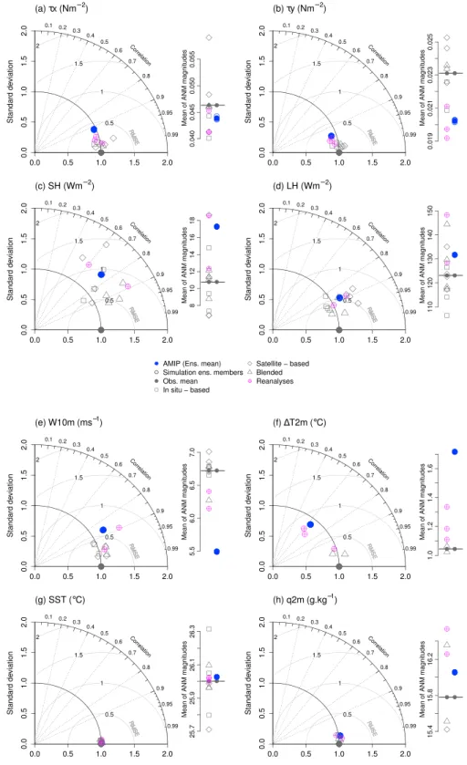
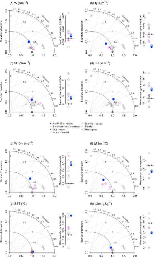
Figure 2. Taylor diagrams representing the annual mean spatial variability over the intertropical oceans relative to
the observational ensemble mean data set for the individual observational data sets and the AMIP simulations for (a) zonal wind stress, (b) meridional wind stress, (c) sensible heat flux, (d) latent heat flux, (e) near-surface wind speed; (f ) sea-air temperature contrast; (g) sea surface temperature, and (h) near-surface specific air humidity. These diagrams show, for each individual data set, three statistics of its spatial distribution relative to the reference: the correlation coefficient (equation (A1) in Appendix A; represented by the azimuthal position on the diagram), the standard deviation (equation (A2) in Appendix A; radial distance from the origin) and the root-mean-square difference (equation (A3) in Appendix A; distance from the reference). Side bars compare the absolute climatological annual mean values averaged over the region between individual observational/model data sets and the reference.
Since the degree of agreement among products in terms of mean variable magnitudes is not necessarily correlated with the agreement in terms of their variability patterns, we go one step further and disconnect the typical magnitudes from the spatial patterns by decomposing the annual mean data at every grid point into a mean value over the tropics⟨xij⟩ and an annual mean spatial pattern (the spatial anomaly from the spatial mean)𝛿xijfor every product:
xij=⟨xij⟩ + 𝛿xij (7)
We synthesize, for each climatological annual mean data set x, three statistics of its spatial variability relative to that of the observational reference over the intertropical oceans with the aid of the Taylor diagrams in Figure 2 [Taylor, 2001]. Details on notation and statistics can be found in Appendix A. Figure 2 also contains information on the mean magnitudes of the variables in the different products, by comparing the spatial averages of their absolute values over the intertropical oceans,⟨|xij|⟩, along the side bars next to the Taylor diagrams.
Finally, we also consider the seasonal variability around the annual mean, separately, by decomposing the climatological monthly data at every grid point xijtinto its annual mean component, xijand a local seasonal
anomaly𝛿xijtthat we treat separately:
xijt= xij+𝛿xijt (8)
We summarize the information related to the climatological seasonal variations𝛿xijtin a similar fashion to the analysis of the annual mean spatial patterns in Figure 3. For the spatiotemporal variability we consider the 12 months in the calculation of the correlation and RMS. The side bars compare the average amplitudes of the climatological seasonal cycle over the intertropical region,⟨OBSSA⟩, where OBSSAis defined at each grid point as the difference between the maximum and minimum climatological monthly data.
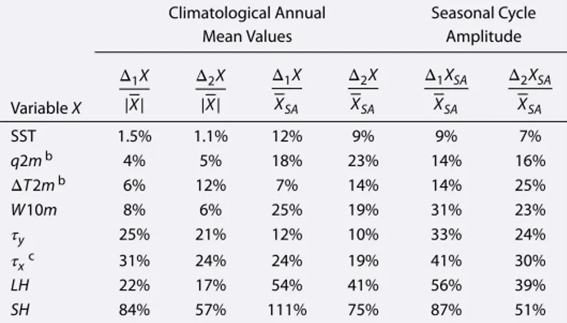
To fully assess how large the average uncertainty is, we compared the different spreads with two physically relevant magnitudes: the average climatological annual mean magnitude and the average amplitude of the climatological seasonal cycle of the mean reference OBS. These averages are representative of a mean value over the tropics. These relative measures are presented in Table 3.
In the following subsections, we present the results of these analyses for the different variables: the wind stress (3.2), the turbulent heat fluxes (3.3), and the meteorological state variables associated to the turbulent fluxes (3.4).
3.2. Wind Stress
The maps of the ensemble mean zonal and meridional wind stress in Figures 1a1 and 1b1 are consistent with the well-known features of the wind stress at low latitudes. The tropics are characterized by a predominantly easterly wind stress over the oceans, with maxima located near the central regions of the basins (Figure 1a1). Weak westerly wind stress is found over limited areas such as the Arabian Sea and Bay of Bengal, where it is associated to the annual reversal of the monsoon circulation. The weaker equatorward component of the wind stress, with climatological annual mean values on the order of 0.02 N m−2(versus 0.05 N m−2for𝜏
x), is
maximal along the continental west coasts, where the wind stress field is influenced by orography (Figure 1b1). The colors in Figures 1a2 and 1b2 show the maximum departures of the different products from the ensemble mean (the “maximum observational uncertainty,” as defined in section 2.3, equation (4)) for the climatological annual mean zonal and meridional components of the wind stress. The annual mean climatological zonal wind stress𝜏xhas maximum uncertainties of 0.014 ± 0.007 N m−2over the intertropical oceans (note that statistics
are given as mean ± standard deviation of climatological annual mean values over the intertropical oceans domain throughout the text, unless otherwise specified). Consistent with the lower magnitudes of𝜏y, the𝜏y
uncertainties are smaller (0.006 ± 0.003 N m−2), especially over the central west tropical and subequatorial
oceanic regions (Figure 1a2). Note, however, that relative to their respective average magnitudes, the Δ1OBS
uncertainties in the two components of the wind stress are rather similar: 25% for𝜏yand 31% for𝜏x(Table 3).
The typical distances between the different wind stress products, Δ2OBS(equation (6)) are given by the
contours in Figures 1a2 and 1b2. These pairwise RMS observational uncertainty estimates show roughly the same spatial patterns over the tropics as the maximum uncertainties Δ1OBS, but are lower, on the order of
Figure 3. Taylor diagrams representing AMIP-modeled and observational climatological seasonal variability over the
intertropical oceans relative to the observational ensemble mean data set (same as equations (A1), (A2), and (A3),
Appendix A, with𝛿xijt,𝛿OBSijt,NiNjNtinstead of𝛿xij,𝛿OBSij,NiNj, respectively, and summation on all three dimensions
i,j, andt), for (a) zonal wind stress, (b) meridional wind stress, (c) sensible heat flux, (d) latent heat flux, (e) near-surface
wind speed, (f ) sea-air temperature contrast, (g) sea surface temperature, and (h) near-surface specific air humidity. Side bars compare the spatial averages of the local amplitudes of the climatological seasonal cycle between individual observational/model data sets and the reference.
Table 3. Observational Uncertainty Divided by the Observational Ensemble
Mean Magnitudes|X|or by the Amplitude of the Ensemble Mean
Climatological Seasonal CycleXSAa
Climatological Annual Seasonal Cycle
Mean Values Amplitude
Variable X Δ1X |X| Δ2X |X| Δ1X XSA Δ2X XSA Δ1XSA XSA Δ2XSA XSA SST 1.5% 1.1% 12% 9% 9% 7% q2mb 4% 5% 18% 23% 14% 16% ΔT2mb 6% 12% 7% 14% 14% 25% W10m 8% 6% 25% 19% 31% 23% 𝜏y 25% 21% 12% 10% 33% 24% 𝜏xc 31% 24% 24% 19% 41% 30% LH 22% 17% 54% 41% 56% 39% SH 84% 57% 111% 75% 87% 51%
aValues are given as percentages of spatially averaged terms over the
intertropical oceans. The variables are presented in ascending order of uncer-tainty. Note that reanalysis products were excluded from the calculation of these statistics.
bDue to the reduced availability of products for these variables, the statistics
presented here are likely (potentially serious) underestimates of the present
uncertainty inq2mandΔT2mfields associated to surface flux products. The
restricted number of products is also the reason for the superiority of the pair-wise uncertainty estimates to those based on the maximum departure from the ensemble mean.
cNote that IFREMER𝜏
xcould be considered an outlier in this data collection.
If it was excluded from the statistics, these values would become, in order, 21%, 17%, 17%, 13%, 29%, and 24%.
The wind stress uncertainty ranges issued from this intercomparison are slightly narrower than the ones reported by Smith et al. [2011] for zonal wind stress. This is possibly due to the use of updated data products and our exclusion of the reanalyses from the estimate of observational spread.
The Taylor diagrams in Figures 2a and 2b show that the correlation coefficient between the spatial variations of the individual climatological wind stress products and the ensemble observational mean exceeds 0.98 for both𝜏x and𝜏y. The different observational annual mean wind stress data sets thus agree reasonably well in terms of their spatial patterns. They also agree well on the𝜏x,𝜏ygradients, as their respective standard
deviations do not differ by more than 10% from𝜎s,OBSfor both wind stress components (except for one𝜏x
product, which we discuss at the end of this subsection).
Figure 4 offers a glimpse of the climatological zonal wind stress seasonality. Intertropical seasonal variations differ spatially not only in terms of amplitude (e.g., Figure 4a) and timing but also in terms of shape, as some regions are characterized by an annual cycle (e.g., Figure 4b), while others show semiannual variations (e.g., Figure 4c). The amplitude of the climatological seasonal cycle is very large compared to the average annual mean magnitudes, OBSSAbeing on the order of 0.06 N m−2for𝜏
x(Figures 4a and 3a) and 0.05 N m−2for𝜏y
(Figure 4b). The maximum differences between the different products and the observational mean estimate represent 41% and 33% of the mean values of the climatological seasonal cycle amplitude for the two components of the wind stress, while the pairwise differences represent 30% and 24%, respectively (Table 3). The agreement between the wind stress products for the climatological seasonal cycle (Figures 3a and 3b) is similar to that found for the annual mean distributions (Figures 2a and 2b). The similar standard deviations and the high correlation coefficients with the common reference for𝛿𝜏ijtand𝛿𝜏ijhighlight robust observational estimates of the climatological spatial patterns and seasonality of wind stress. The only exception is the IFREMER zonal wind stress product (outlier diamond symbol on Taylor diagrams and side bars of Figures 2a and 3a). Despite very similar 𝜏y estimates to the other products, the IFREMER satellite product shows
Figure 4. (a) Amplitude of the climatological seasonal cycle of the observational mean surface zonal wind stress,𝜏x;
(b) and (c) observational and simulated climatological seasonal cycles of𝜏x, averaged over two regions of the same size
in the West Pacific warm pool (PWP: 125◦E–185◦E, 5◦N–15◦N) and in the East equatorial Pacific (NINO3: 210◦E–270◦E,
5◦S–5◦N), respectively.
and higher climatological seasonal cycle amplitude and variability (Figure 3a). A recent, fully revised, version of the IFREMER product [Bentamy et al., 2013] may offer an improved agreement with the other𝜏xestimates.
3.3. Heat Fluxes
With an order of magnitude of 10 W m−2over the intertropical oceans (Figure 1c1), the sensible heat flux is a
weak (∼ 8%) component of the total ocean-atmosphere turbulent heat flux in these regions. It is tightly linked with the ocean-lower atmosphere temperature contrast and the wind speed (equation (3)). SH is thus positive (heat flux from the ocean to the atmosphere) for most of the tropics and presents low or even negative values above oceanic upwelling regions where the shoaling of the thermocline brings cold seawater to the surface (e.g., Pacific equatorial upwelling—Figure 1c1).
The spread between the 13 estimates of SH considered is comparatively very high. Maximum differences of 9 ± 3 W m−2(Figure 1c2) between individual estimates and the observational mean are almost as large as
the climatological mean values of the flux themselves (Figure 1c1) and exceed the amplitude of the mean climatological seasonal cycle (Table 3). IFREMER and JRA25 provide the highest, and Da Silva and J-OFURO2 the lowest estimates of the ensemble (highest and lowest two symbols on the side bar of Figure 2c). Pairwise differences among products show a similar distribution of lower/higher uncertainty regions (contours versus colors in Figure 1c2) and are roughly 30% lower than the Δ1OBSestimates. As shown in Figures 2c and 3c, the
seasonality and spatial patterns are also very poorly correlated between the different products, with correla-tion coefficients ranging from 0.5 to 0.97. The regions of highest uncertainty correspond to a large degree to strong wind stress regions (Figures 1c2, 1a1, and 1b1).
Most of the turbulent heat exchanged between the ocean and the atmosphere in the tropics is in the form of latent heat. The observational annual mean climatological latent heat flux (Figure 1d1) is on the order of 122 ± 27 W m−2. The associated pattern carries the signature of the cold surface waters in upwelling regions,
resulting in low latent heat fluxes, as well as that of the near-surface wind speed (equation (2) and Figure 1e1). The 13 latent heat flux data sets agree somewhat better on spatial patterns and seasonal variability than the corresponding sensible heat flux estimates (Figures 2d and 3d versus Figures 2c and 3c). However, the maximum deviation between individual products and the observational mean is 27 ± 6 W m−2(Figure 1d2),
Figure 5. Distributions of the values of climatological monthly 10 m
level wind speeds over the intertropical oceans in: AMIP simulations (blue: solid line - ensemble mean; dotted lines - ensemble members) and different observational data sets (other colors).
roughly equivalent to 54% of the average climatological seasonal cycle ampli-tude of sea-air LH at low latiampli-tudes (Table 3). Comparatively, the pairwise differences between the climatological annual mean LH products are equivalent to roughly 41% of the mean tropical sea-sonal amplitude OBSSA (Table 3). JRA25
and DFS4 give the highest estimates of the latent heat flux (side bar, Figure 2d), while the lowest estimates are given by FSU3 and, except for some oceanic upwelling regions, the Da Silva data sets. Despite a better agreement between the
LH than between the SH products, there
is still a large spread in the amplitude and even shape of the mean seasonal cycle of LH, with some observational data sets differing by as much as 56% from the ensemble mean in terms of average sea-sonal cycle amplitude over the intertrop-ical oceans (Table 3). Interestingly, the regions of highest uncertainty on the latent heat flux seasonal cycle amplitude coincide to a large extent to those of the sensible heat flux (not shown). A considerable spread is also found between the spatial dis-tributions of the latent heat flux (Figure 2d), with individual observational LH patterns showing correlation coefficients with the observational mean over the entire study field from 0.97 down to 0.82, and much less in certain regions.
3.4. Uncertainties in Temperature, Wind, and Humidity
Much like the surface wind stress, the 10 m level wind speed patterns and seasonal variations agree reasonably well between the different observational products (Figures 2e and 3e). However, the spread in absolute values (Δ1OBSon the order of 0.6 ± 0.2 m s−1) corresponds to approximately 25% of the mean amplitude of the
climatological seasonal variations (Table 3). Figure 5 summarizes the distribution of climatological monthly wind speed values in the different data sets when considering all grid points over the intertropical oceans. It is notable that the reanalysis products and TropFlux (pink dashed and similar grey dotted curves in Figure 5) tend to provide lower estimates of the near-surface wind speed for most regions over the intertropical oceans and contain several occurrences of very low climatological monthly wind speed values (W10m < 3 m s−1).
Such low climatological values are absent from the other data sets. Another notable observation is that NCEP contains considerably more spatial variability than all the other data sets (visible as the isolated reanalysis product with the highest normalized standard deviation in Figure 2e). No such signature is found, however, for the NCEP wind stress components (Figures 2a and 2b). Likewise, the outstanding characteristics of the IFREMER𝜏xclimatology noted in section 3.2 are not reflected in the comparison of the corresponding wind speed field with the other W10m products.
Only five of the data sets we have considered provided both the sea surface temperature and the 2 m level air temperature, allowing the computation of the sea-air temperature contrast (Table 2). Out of these, the non-reanalysis products, TropFlux and DFS4, are in good agreement on the values, mean patterns and seasonal variations of ΔT2m (Table 3 and Figures 2f and 3f ). On the other hand, the reanalysis products show important departures from the two blended data fields. JRA25 and ERA-Interim present higher mean ΔT2m magnitudes (side bar, Figure 2f ), and the spatial and seasonal variability in NCEP/NCAR and JRA25 presents much lower correlations with the ensemble mean than the other three products (Figures 2f and 3f ). The reduced number of non-reanalysis data sets has the effect of reversing the relationship we have seen so far between the two uncertainty estimate types, with Δ1OBS < Δ2OBSfor ΔT2m, as the “typical distance” between the two data sets becomes necessarily superior to their “maximum departure from the mean” (Table 3).
Among the variables considered in this study, the sea surface temperature is the best constrained (Table 3), with the 11 observational data sets agreeing on the large-scale patterns (Figure 2g) as well as on the seasonal variability (Figure 3g and Table 3). FSU3 is markedly warmer than all the other data sets, while HOAPS3 and the Da Silva climatology give the coldest estimates of the sea surface temperature.
Although to a very large extent covarying with the sea surface temperature, the 2 m level specific air humidity shows relatively more spread in magnitudes between the three available non-reanalysis observational fields (Table 3). Out of these, HOAPS3 and DFS4 provide consistently lower humidity estimates (not shown) than TropFlux, and also than NCEP/NCAR and JRA25. HOAPS3 also has a different statistical distribution of clima-tological intertropical q2m values compared to the reanalysis and blended products, with less high and more intermediate values (not shown). This corresponds to a westward extension of the relatively dry regions over the eastern subequatorial ocean basins in HOAPS3 compared to the other climatologies. Correlations with the observational mean larger than 0.97 indicate that the different q2m products agree well in terms of spatial and seasonal variation patterns (Figures 2h and 3h). However, a 14% spread in the mean amplitude of the seasonal cycle exists between the three non-reanalysis q2m products considered (Table 3). The spatial distribution of this uncertainty (not shown) matches that of the latent heat flux.
Note that the data sets associated to the highest (JRA25) and lowest (FSU3) estimates of the latent heat flux do not have extreme estimates of the (available) corresponding surface state variables that would explain the LH values. Together with the lack of wind speed-wind stress correspondence for the outstanding characteristics of IFREMER 𝜏x and NCEP W10m within the observational ensemble, this indicates a disjunction of the climatological magnitudes of the turbulent surface fluxes and flux-related state variables among the different products.
3.5. Systematic Differences Between Flux Product Types?
We further assess whether we can identify systematic differences between the different flux product types, i.e., in situ, satellite, blended, and reanalyses.
The four satellite-based latent heat flux products carry a particular spatial pattern signature (not shown). This consists of amplified fluxes (compared to the observational mean distribution) along tropical east to equa-torial west diagonals over the Atlantic and Pacific basins, around 20–30◦S in the Indian Ocean and over the Arabian Sea. These regions roughly coincide with the regions of strong zonal wind stress visible in Figure 1a1. This pattern is responsible for the high spatial variability of the satellite-based LH products visible in Figure 2d. Only two of the satellite products (IFREMER and HOAPS3) show the same signature in their SH fields. The reanalyses also carry a common specificity in their LH and SH spatial patterns (not shown), consisting of exaggerated heat flux values off the subequatorial and tropical west coasts of Africa, North America, and South America. This feature is more pronounced for JRA25 than for NCEP/NCAR. Ignoring a mean shift toward low flux magnitudes for LH, this pattern is also somewhat present in the TropFlux heat fluxes and might be linked to the atmospheric stability formulation in the flux bulk formula. In turn, this could respond to a weak representation of stratocumulus clouds, a classical problem of many current atmospheric models.
With the few exceptions noted above, which are not strictly category specific, we did not detect any category-based clustering of the different types of observational products, either in terms of magnitudes or large-scale statistics describing the spatial patterns and seasonal variations. Furthermore, even though they tend to provide somewhat lower W10m and higher ΔT2m estimates than most observational products and while often commented out of the surface flux observational product suite, atmospheric reanalyses seem to provide intertropical turbulent air-sea fluxes comparable to the other products we have analyzed—except for the aforementioned coastal bias.
4. Air-Sea Flux Representation in the IPSL CMIP5 AMIP Simulations
In this section we use the previously described observational ensemble to analyze how the sea-air turbulent fluxes and associated state variables (equations (1)–(3)) are represented in LMDZ5A, in light of the observational spread. Our objective is to identify and draw attention to the robust, important large-scale flux-related errors in the model climatology. Thus, rather than looking for a skill score, we assess if the model results are within or outside the range covered by the different observational products.
Figure 6. AMIP simulated climatological annual mean (a1) zonal wind stress, (b1) meridional wind stress, (c1) sensible
heat flux, (d1) latent heat flux, (e1) near-surface wind speed, (f1) sea-air temperature contrast, (g1) sea surface temperature, (h1) near-surface specific air humidity over the intertropical oceans, and (a2–h2) the associated model-mean observations differences; the dotted regions correspond to areas where the model bias is not considered significant relative to the maximum observational spread—see text for details.
4.1. Model Evaluation Strategy
We build on the analyses used to describe the observational ensemble (section 3.1) to show how the model compares to it. Following this, we first look at the climatological annual mean fields of the model ensemble mean AMIP, in Figures 6a1–6h1. The mean model biases with respect to the different observational data sets ΔAMIP are shown in colors in Figures 6a2–6h2. For a “maximum model bias” estimate Δ1AMIPcomparable to Δ1OBS(equation (4)), we consider the maximum absolute value of the difference between each individual
AMIP simulation and the mean observational reference. The regions not dotted in Figures 6a2–6h2 indicate “significant” model biases, defined as those grid points where Δ1AMIP > Δ1OBS. Details on these statistics
can be found in Appendix B. Alternative definitions of significant model biases are possible. The Δ1criterion is
the most suited to our present goal and is thus used in Figures 6a2–6h2 and Table 4. However, for comparison, we have also devised an alternative criterion using Δ2OBS (equation (6)) and RMS differences between all AMIP-OBS combinations. We briefly present this parallel assessment in Appendix C. The results of this alternative analysis are very similar to the results presented below, using the Δ1 criterion, except for the sensible heat flux, where the Δ2 criterion results in a much larger area where the model bias is
considered significant.
As for the description of the observational ensemble, we use the Taylor diagrams and their side bars (Figure 2) to show how the model compares to the observational ensemble mean for the mean magnitudes over the tropics and the spatial variability of the annual mean fields (equation (7)). The same is done for the characterization of the seasonal variability (equation (8); results in Figure 3).
Taking advantage of the availability of the ensemble of AMIP historical simulations, we have also analyzed the differences introduced by the internal variability, regarded as noise, in the atmospheric model. We have found them to be invariably negligible compared to the differences between the model results and the observational mean, for all of the variables considered. Results for these individual model realizations are plotted in Figures 2–5.
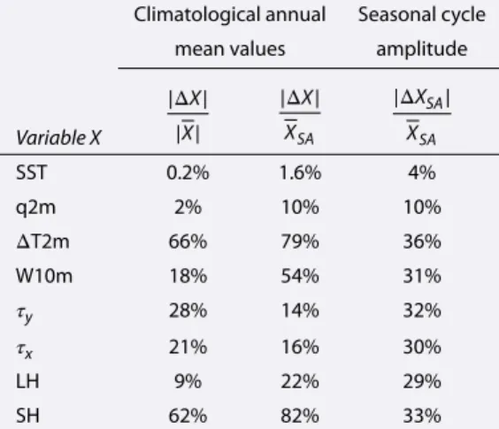
Table 4. Summary of Mean Statistics Over the
Intertropical Oceans Comparing the AMIP Simulation
Results to the Observational Meana
Climatological annual Seasonal cycle
mean values amplitude
Variable X |ΔX| |X| |ΔX| XSA |ΔXSA| XSA SST 0.2% 1.6% 4% q2m 2% 10% 10% ΔT2m 66% 79% 36% W10m 18% 54% 31% 𝜏y 28% 14% 32% 𝜏x 21% 16% 30% LH 9% 22% 29% SH 62% 82% 33%
a|ΔX|is the spatial average of the model bias
mag-nitudes|ΔAMIP|(equation (B2) in Appendix B) for the
annual mean values of variableXover the
intertrop-ical oceans;|X|and XSAare the spatial averages of
the annual observational ensemble mean magnitudes
|OBS| and of the observational climatological
sea-sonal cycle amplitudeOBSSA, respectively (see text in
section 3.1 for details);|ΔXSA|is the spatially averaged
magnitude of the climatological seasonal cycle
ampli-tude biasΔAMIPSA(equation (B4) in Appendix B). Note
that reanalysis products were excluded from these statistics.
It should be noted that the Program for Climate Model Diagnosis and Intercomparison SST data set [Taylor et al., 2000] used to force the AMIP simulations is well within the observational envelope, close to the observational mean in terms of magnitude and spatial variability (blue symbol in Figure 2g). We thus argue that the choice of this SST data set for the AMIP forcing should not be responsible for biases on other variables (following our evaluation approach), at least on the magnitude and spatial variability of the climatological annual mean.
4.2. Wind Stress
Using prescribed observational SSTs, the atmospheric model produces a generally good representation of the climatological wind stress (Figures 2a and 2b). However, some significant biases do emerge in the annual mean pattern over certain regions and can take both positive and negative values. The wind stress is underestimated, for example, over the Arabian Sea and the Bay of Bengal, and overestimated along tropical east to equatorial west diagonals in the South Pacific and Atlantic Oceans (Figures 6a2 and 6b2). Addition-ally, compared to the mean observations, the simu-lated𝜏yexhibits a somewhat weaker and wider
conver-gence region in the Pacific and Atlantic Oceans around 5–7◦N (Figures 6b1 and 6b2), while the simulated𝜏x
results show a narrower band of trade winds located too far north in the equatorial Pacific (Figures 6a1 and 6a2). The decomposition in Figures 2a and 2b shows that wind stress component average magnitudes over the intertropical oceans are within the estimates from the different wind stress products, whereas the bias patterns are significant. The model shows a larger RMS difference from the mean observational reference than any of the observational products. This reflects small pattern shifts (low correlation) rather than a difference of spatial variability amplitude (Figures 2a and 2b)
These patterns are consistent with the 10 m level wind speed bias patterns (Figure 6e2), as can be expected from equation (1). However, the simulated wind speed values are systematically lower than observed over most of the tropics (Figure 6e2). The mean wind speed bias of the model over the intertropical oceans is 1.2 ± 0.5 m s−1, equivalent to 18% of the observed annual mean W10m (Table 4). Furthermore, the
probability distribution functions of climatological monthly W10m in Figure 5 shows that the model simulates consistently lower wind speeds than observed. Some climatological values are lower than the minimum observational climatological values (down to 2 m s−1), and the model presents a much higher
occur-rence of wind speeds between 2 and 4 m s−1than in most observations. Interestingly, the only observational
data sets that contain such low climatological wind speed values are the reanalyses and the hybrid product TropFlux. These are the same products that have a similar statistical distribution of climatological W10m with the model (Figure 5) and a remarkably similar spatial pattern when compared to the observational mean refer-ence (not shown, but similar to Figure 6e2). This suggests potentially similar behaviors of the LMDZ5A model and of the atmospheric models used in the generation of these products.
At the seasonal time scale, the simulated climatological seasonal cycle amplitude over the intertropical oceans is close to the mean observational value for𝜏x (side bar, Figure 3a; 0.061 ± 0.036 N m−2simulated versus
0.059 ± 0.040 N m−2observed), whereas it is underestimated for𝜏
y(Figure 3b; 0.042 ± 0.034 N m−2simulated
versus 0.048 ± 0.037 N m−2observed𝜏
yamplitude). Despite the good large-scale agreement (Figure 3a),
significant regional biases in terms of seasonal cycle amplitude are found for𝜏x. For example, it exhibits an amplified seasonal cycle in the NINO3 region (210◦E–270◦E, 5◦S–5◦N, Figure 4c), which, in a coupled model, could have repercussions on the representation of the Pacific equatorial upwelling and the El Ni ˜no–Southern Oscillation (ENSO) variability. In the West Pacific warm pool (e.g., 125◦E–185◦E, 5◦N–15◦N), the seasonality of
𝜏xis slightly underestimated, which is mostly due to relatively low𝜏xvalues during boreal summer (Figure 4b).
These biases represent about 30% of the seasonal amplitude at the tropical scale (Table 4). Differences in local timing and shape of the seasonal cycle translate into degraded correlations and RMS differences in Figure 3a and 3b compared to similar estimates for the annual mean patterns in Figure 2. These seasonal differences in wind stress have their counterpart in the seasonal variability of the wind speed (Figure 3e).
4.3. Sensible Heat Flux
The AMIP SH values fall on the high end of, but within the observational range (Figure 2c). Notable excep-tions where the sensible heat flux is overestimated even compared to the highest observational data are the eastern boundaries of the Atlantic and Pacific basins between approximately 10◦and 30◦S and 10◦and 30◦N (Figures 6c2 and 6c1). These bias regions are very similar to those found in reanalyses, indicating a potentially similar source of error in different atmospheric models.
Despite the model underestimated near-surface wind speed, the simulated annual mean SH exceeds by 7 ± 3 W m−2, or roughly 62% (Table 4), the annual observational average. This is due to a consistent,
sig-nificant overestimation (on the order of 66%, Table 4) of the sea-air temperature contrast over the entire intertropical oceans domain (Figure 6f2). Both the climatological value and bias SH patterns match those of ΔT2m (Figures 6c1, 6f1, 6c2, and 6f2). A modulation of the sensible heat flux by the near-surface wind speed is, however, present, for example, in the east equatorial Atlantic and Pacific, and the Indo-Pacific warm pool region, where the accentuated negative wind speed bias partially compensates the overestimated ΔT2m (Figures 6c2, 6e2, and 6f2).
4.4. Latent Heat Flux
Similarly, despite a generally good representation of q2m (as a result of its tight coupling with the imposed SST—Figures 6h2, 6h1, and 6g1) and the underestimated W10m, the climatological latent heat flux values are in many regions in the upper quartile of the observational products. The differences between the simulated and the observational mean latent heat fluxes are physically important (11 ± 8 W m−2), but they
are not significant for most regions considering the large spread of observational values (Figure 6d2). Large-scale statistics of LH over the intertropial oceans (Figures 2d and 3d) only distinguish the model from the observations for the seasonality patterns (Figure 3d). In particular, the slightly lower correlation with the mean observational reference (rt,AMIP= 0.86) than the individual observational climatologies (rt,OBSbetween 0.88 and 0.97) indicates slightly less agreement with the observations on the timing and/or collocation of the seasonal variations.
The pattern of the difference between AMIP and the OBS LH data set is dominated by the wind speed bias pattern. Overestimated latent heat fluxes primarily correspond to regions of relatively overestimated wind speed (with respect to the mean, negative, W10m bias) and vice-versa (Figures 6d2 and 6e2). However, some effects of the weak humidity bias are visible in the latent heat flux representation (Figures 6d2 and 6h2). One such effect consists of horseshoe patterns of slightly overestimated humidity in the Indian and intertropical Pacific Oceans leading to relatively lower latent heat fluxes. Likewise, drier than observed conditions in the eastern equatorial Atlantic and, to a smaller extent, Pacific regions drive relatively high latent heat fluxes in these areas, despite a severe underestimation of the collocated wind speeds (Figures 6d2, 6e2, and 6h2).
5. Summary and Discussion
The present study serves the evaluation of turbulent fluxes in the atmospheric component of the IPSL-CM5A model. In this context, we have assembled a database of 14 climatological surface flux products (Table 1) to be used for large-scale model evaluation of turbulent ocean-atmosphere interactions in the intertropical zone (30◦S–30◦N). This database spans four different categories of flux products—in situ, satellite based, atmo-spheric reanalysis, and blended—and includes climatological monthly fields of the turbulent momentum and heat fluxes, as well as of the associated surface state variables (Table 2).
We treated this database as an observational ensemble and estimated the observational spread in two different ways, considering both the state variables and turbulent fluxes over a climatological annual cycle computed from nearly three decades with maximum data coverage (1979–2005).
Overall, the spatial distributions of the two observational spread estimates are very similar (colors versus contours in Figures 1a2 to 1h2), while their magnitudes can differ substantially. The typical distance between
two products (Δ2OBS) is generally smaller than the maximum departure from the observational mean (Δ1OBS), except for situations where they are calculated from very few observational products (e.g., two
products for ΔT2m and three products for q2m in this study). In the latter case, the different products tend to be all similarly far from the ensemble mean and the typical pairwise distance between them becomes superior to the maximum distance to the ensemble mean. The two measures of observational spread offer complementary information and the choice of any one observational uncertainty estimate depends on the application.
As expected, SST was found to be the most reliable variable, with the spread of the mean values approximately equivalent to 1.5% of the average absolute values and 12% of the average climatological seasonal cycle amplitude. Only moderately higher relative uncertainties have been found among these products for q2m and ΔT2m. However, since we excluded reanalyses, these uncertainties have been estimated based on three data sets for q2m and only two data sets for ΔT2m. They could thus be underestimates of the current uncertainty in these fields. Wind speed and wind stress uncertainties have been found to be close to the target accuracies suggested by Gulev et al. [2010] for many climatological applications: below 1 m s−1for wind speed
and below 0.01 N m−2for the meridional and for the zonal wind stress, if the IFREMER𝜏
xproduct is excluded.
Large uncertainties that hinder the full assessment of climate model results have been found for the turbulent surface heat fluxes both for the annual mean and the seasonal cycle, a problem already highlighted by other studies [Wittenberg et al., 2006; Reichler and Kim, 2008]. While a target accuracy in the individual heat flux components is on the order of 2–3 W m−2[Gulev et al., 2010], and biases larger than 10 W m−2are considered
serious problems in climate studies [WCRP, 1989; Bourassa et al., 2008] average uncertainties on the order of 10 W m−2and 30 W m−2have been found for the sensible and latent heat fluxes, respectively. The uncertainties
are of the same order of magnitude as the climatological SH values and represent 20% and 50% of the average LH annual mean value and climatological seasonal cycle amplitude, respectively. These results show that important efforts are still needed to progress toward a consensus on low-latitude heat flux estimates. The same ranking among the variables in terms of spread between products has been found for the spatial variations around the mean. The exception was a surprisingly good agreement between the different products in terms of the spatial variations of the wind stress components, given a lower agreement in wind speed patterns (Figures 2a, 2b, and 2e).
A larger spread has been found among products when considering the amplitudes of the climatological seasonal cycles compared to that between the annual mean values, with a common ranking of the variables according to their respective observational uncertainty. Meanwhile, the shapes of the seasonal cycles were as well or even better correlated between the different observational products than the respective annual mean spatial patterns (Figure 3 versus Figure 2). In addition, the seasonal cycle amplitude uncertainties of the sensible heat flux, latent heat flux, and air humidity share a common spatial distribution.
When comparing in situ-based, satellite-based, hybrid, and reanalysis products, the only category-specific characteristic detected was a common tendency of satellite products to show particularly enhanced latent heat fluxes (and sensible heat fluxes, for two of the products) in regions roughly coinciding with the strong𝜏x regions in Figure 1a1, compared to the LH patterns of the other observational data sets.
At the large scale, only two of the analyzed observational climatologies (Table 2) may be qualified as outliers: the IFREMER zonal wind stress, for its high spatiotemporal variability and absolute annual mean values, and the NCEP/NCAR 10 m level wind speed, for its large spatial gradients. None of these outstanding characteristics is reflected in the other associated variables. Similar findings for other products indicate that no flux product can be excluded on the basis of a systematic bias in its ancillary data. Note that, despite having been proven outdated in what concerns data coverage and energy balance, for the large-scale criteria chosen in this analysis the Da Silva climatology fits well within the described observational ensemble.
In showing that there are no clear separations between the different flux product types in terms of their features and that there are no systematic outliers, this comparison supports the use of this wide array of observational products as an ensemble for large-scale model validation. Using this approach, we were able to analyze the LMDZ5A atmospheric simulation results in light of the observational spread and to identify its significant biases.
We show that LMDZ5A develops two important biases related to turbulent ocean-atmosphere exchanges across the intertropical region. First, 10 m level wind speeds are consistently underestimated, on average by