Minimization of an energy error functional to solve a Cauchy problem arising in plasma physics: the reconstruction of the magnetic flux in the vacuum surrounding the plasma in a Tokamak

HAL Id: hal-00481257

https://hal.inria.fr/hal-00481257v2

Submitted on 7 Apr 2016 (v2), last revised 17 Nov 2013 (v3)

HAL is a multi-disciplinary open access

archive for the deposit and dissemination of

sci-entific research documents, whether they are

pub-lished or not. The documents may come from

teaching and research institutions in France or

L’archive ouverte pluridisciplinaire HAL, est

destinée au dépôt et à la diffusion de documents

scientifiques de niveau recherche, publiés ou non,

émanant des établissements d’enseignement et de

recherche français ou étrangers, des laboratoires

Minimization of an energy error functional to solve a

Cauchy problem arising in plasma physics: the

reconstruction of the magnetic flux in the vacuum

surrounding the plasma in a Tokamak

Blaise Faugeras, Amel Ben Abda, Jacques Blum, Cédric Boulbe

To cite this version:

Blaise Faugeras, Amel Ben Abda, Jacques Blum, Cédric Boulbe. Minimization of an energy error

functional to solve a Cauchy problem arising in plasma physics: the reconstruction of the magnetic

flux in the vacuum surrounding the plasma in a Tokamak. Revue Africaine de la Recherche en

Informatique et Mathématiques Appliquées, INRIA, 2012, 15, pp.37-60. �hal-00481257v2�

solve a Cauchy problem arising in plasma

physics: the reconstruction of the magnetic

flux in the vacuum surrounding the plasma in

a Tokamak

Blaise Faugeras

_{Amel Ben Abda}

_{Jacques Blum}

_{Cedric Boulbe}

06108 Nice Cedex 02, France Blaise.Faugeras@unice.fr ** ENIT-LAMSIN, BP 37, 1002 Tunis, Tunisie Amel.BenAbda@enit.rnu.tn

RÉSUMÉ. Une méthode numérique de calcul du flux magnétique dans le vide entourant la plasma

dans un Tokamak est étudiée. Elle est basée sur la formulation d’un problème de Cauchy qui est ré-solu en minimisant une fonctionnelle d’écart énergétique. Différentes expériences numériques montrent l’efficacité de la méthode.

ABSTRACT. A numerical method for the computation of the magnetic flux in the vacuum surrounding

the plasma in a Tokamak is investigated. It is based on the formulation of a Cauchy problem which is solved through the minimization of an energy error functional. Several numerical experiments are conducted which show the efficiency of the method.

MOTS-CLÉS : EDP elliptique, problème inverse, écart énergétique, plasma, Tokamak KEYWORDS : Elliptic PDE, inverse problem, energy error, plasma, Tokamak

Received,June 19, 2011, Revised, February 2, 2012,

1. Introduction

In order to be able to control the plasma during a fusion experiment in a Tokamak it is mandatory to know its position in the vacuum vessel. This latter is deduced from the knowledge of the poloidal flux which itself relies on measurements of the magnetic field. In this paper we investigate a numerical method for the computation of the poloidal flux in the vacuum. Let us first briefly recall the equations modelizing the equilibrium of a plasma in a Tokamak [32].

Assuming an axisymmetric configuration one considers a 2D poloidal cross section of the vacuum vesselΩV in the(r, z) system of coordinates (Fig. 1). In this setting the

poloidal flux ψ(r, z) is related to the magnetic field through the relation (Br, Bz) = 1

r(− ∂ψ ∂z,

∂ψ

∂r) and, as there is no toroidal current density in the vacuum outside the

plasma, satisfies the following equation

Lψ= 0 in ΩX (1)

where L denotes the elliptic operator

L.= −[ ∂ ∂r( 1 r ∂. ∂r) + ∂ ∂z( 1 r ∂. ∂z)] and ΩX = ΩV − ¯ΩP

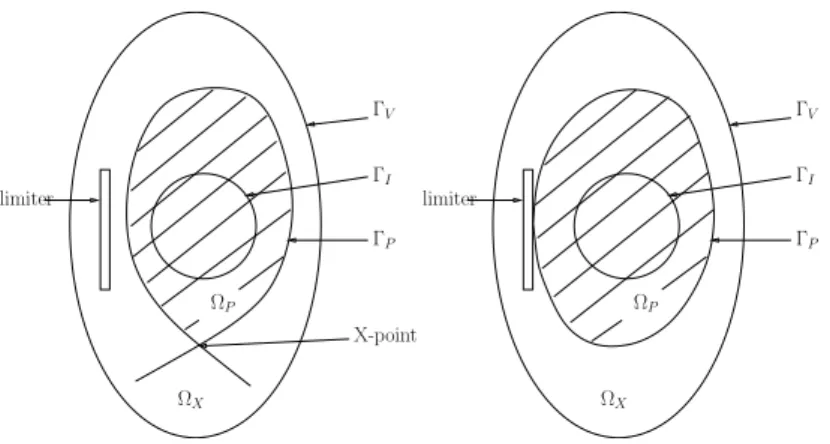
denotes the vacuum region surrounding the domain of the plasmaΩPof boundaryΓP(see

Fig. 2). Inside the plasma Eq. (1) is not valid anymore and the poloidal flux satisfies the Grad-Shafranov equation [30, 16] which describes the equilibrium of a plasma confined by a magnetic field

Lψ= µ0j(r, ψ) in ΩP (2)

where µ0is the magnetic permeability of the vacuum and j(r, ψ) is the unknown toroidal

current density function inside the plasma. Since the plasma boundaryΓP is unknown

the equilibrium of a plasma in a Tokamak is a free boundary problem described by a particular non-linearity of the model. The boundary is an iso-flux line determined either as being a magnetic separatrix (hyperbolic line with an X-point as on the left hand side of Fig. 2) or by the contact with a limiter (Fig. 2 right hand side). In other words the plasma boundary is determined from the equation ψ(r, z) = ψP, ψP being the value of the flux

at the X-point or the value of the flux for the outermost flux line inside a limiter.

In order to compute an approximation of ψ in the vacuum and to find the plasma boundary without knowing the current density j in the plasma and thus without using the Grad-Shafranov equation (2) the strategy which is routinely used in operational codes

z ΓV ΩV coil r O BT BN

Figure 1. Cross section of the vacuum vessel : the domainΩV, its boundaryΓV. Coils

providing measurements of the components of the magnetic field tangent and normal to

ΓV are represented surrounding the vacuum vessel.

ΩX limiter ΓI ΓP X-point ΓV ΩP ΩX limiter ΓI ΓP ΓV ΩP

Figure 2. The plasma domainΩP and the vacuum regionΩX. The plasma boundary is

determined by an X-point configuration (left) or a limiter configuration (right). The fictitious contourΓIis represented inside the plasma.

mainly consists in choosing an a priori expansion method for ψ such as for example trun-cated Taylor and Fourier expansions for the code Apolo on the Tokamak ToreSupra [28] or piecewise polynomial expansions for the code Xloc on the Tokamak JET [26, 29]. The flux ψ can also be expanded in toroidal harmonics involving Legendre functions or expressed by using Green functions in the filament method ([23, 13], [9] and the refe-rences therein). In all cases the coefficients of the expansion are then computed through a fit to the measurements of the magnetic field. Indeed several magnetic probes and flux loops surround the boundaryΓV of the vacuum vessel and measure the magnetic field

and the flux (see Fig. 1). It should also be noted that very similar problems are studied in [18, 8, 14, 15]

In this paper we investigate a numerical method based on the resolution of a Cauchy problem introduced in ([6], Chapter 5) which we recall here below. The proposed ap-proach uses the fact that after a preprocessing of these measurements (interpolation and possibly integration on a contour) one can have access to a complete set of Cauchy data,

f = ψ on ΓV and g=1 r

∂ψ ∂n onΓV.

The poloidal flux satisfies

                   Lψ= 0 in ΩX ψ= f on ΓV 1 r ∂ψ ∂n = g on ΓV ψ= ψP on ΓP (3)

In this formulation the domainΩX= ΩX(ψ) is unknown since the free plasma

boun-daryΓP as well as the flux ψP on the boundary are unknown. Moreover the problem

is ill-posed in the sense of Hadamard [12] since there are two Cauchy conditions on the boundaryΓV.

In order to compute the flux in the vacuum and to find the plasma boundary we are going to define a new problem as in [6] which is an approximation of the original one. Let us define a fictitious boundaryΓIfixed inside the plasma (see Fig. 2). We are going to

seek an approximation of the poloidal flux ψ satisfying Lψ= 0 in the domain contained

between the fixed boundariesΓV andΓI. The problem becomes one formulated on a fixed

domainΩ :            Lψ= 0 in Ω ψ= f on ΓV 1 r ∂ψ ∂n = g on ΓV (4)

Let us insist here on the fact that this problem is an approximation to the original one since in the domain betweenΓP andΓI, ψ should satisfy the Grad-Shafranov equation.

The relevance of this approximating model is consolidated by the Cauchy-Kowalewska theorem [12]. ForΓP smooth enough the function ψ can be extended in the sense of Lψ = 0 in a neighborhood of ΓP inside the plasma. Hence the problem formulated on

a fixed domain with a fictitious boundaryΓI not "too far" fromΓP is an approximation

of the free boundary problem. As mentioned in [6] ifΓI were identical withΓP then by

the virtual shell principle [31] the quantity w = 1 r

∂ψ

∂n|ΓI would represent the surface

current density (up to a factor 1

µ0

) onΓP for which the magnetic field created outside

the plasma by the current sheet is identical to the field created by the real current density spread throughout the plasma.

However no boundary condition is known onΓI. One way to deal with this second

issue and to solve such a problem is to formulate it as an optimal control one. Only the Dirichlet condition onΓV is retained to solve the boundary value problem and a least

square error functional measuring the distance between measured and computed normal derivative and depending on the unknown boundary condition onΓI is minimized. Due

to the illposedness of the considered Cauchy problem a regularization term is needed to avoid erratic behaviour on the boundary where the data is missing. A drawback of this method developed in [6] is that Dirichlet and Neumann boundary conditions onΓV are not

used in a symmetric way. One is used as a boundary condition for the partial differential equation, Lψ= 0, whereas the other is used in the functional to be minimized.

Freezing the domain toΩ by introducing the fictitious boundary ΓI enables to remove

the nonlinearity of the problem. The plasma boundaryΓPcan still be computed as an

iso-flux line and thus is an output of our computations. We are going to compute a function ψ such that the Dirichlet boundary condition u= ψ on ΓIis such that the Cauchy conditions

onΓV are satisfied as nearly as possible in the sense of the error functional defined in the

next Section.

The originality of the approach proposed in this paper relies on the use of an error functional having a physical meaning : an energy error functional or constitutive law er-ror functional. Up to our knowledge this misfit functional has been introduced in [24] in the context of a posteriori estimator in the finite element method. In this context, the minimization of the constitutive law error functional allows to detect the reliability of the mesh without knowing the exact solution. Within the inverse problem community this functional has been introduced in [21, 22, 20] in the context of parameter identification. It has been widely exploited in the same context in [7]. It has also been used for Robin type boundary condition recovering [10] and in the context of geometrical flaws identification (see [4] and references therein). For lacking boundary data recovering (i.e. Cauchy pro-blem resolution) in the context of Laplace operator, the energy error functional has been introduced in [2, 1]. A study of similar techniques can be found in [5, 3] and the analysis

found in these papers uses elements taken from the domain decomposition framework [27].

The paper is organized as follows. In Section 2 we give the formulation of the problem we are interested in and provide an analysis of its well posedness. Section 3 describes the numerical method used. Several numerical experiments are conducted to validate it. The final experiment shows the reconstruction of the poloidal flux and the localization of the plasma boundary for an ITER configuration.

2. Formulation and analysis of the method

2.1. Problem formulation

As described in the Introduction the starting point is the free boundary problem (3). We first proceed as in [6] and in a first step consider the fictitious contourΓI fixed in the

plasma and the fixed domainΩ contained between ΓV andΓI. Problem (3) is

approxi-mated by the Cauchy problem (4). The boundariesΓV andΓI are assumed to be chosen

smooth enough in order not to refrain any of the developments which follow in the paper. In a second step the problem is separated into two different ones. In the first one we retain the Dirichlet boundary condition onΓV only, assume v is given onΓI and seek the

solution ψDof the well-posed boundary value problem :

         LψD= 0 in Ω ψD= f on ΓV ψD= v on ΓI (5)

The solution ψD can be decomposed in a part linearly depending on v and a part

depending on f only. We have the following decomposition :

ψD= ψD(v, f ) = ψD(v, 0) + ψD(0, f ) := ψD(v) + ˜ψD(f ) (6)

where ψD(v) and ˜ψD(f ) satisfy :          LψD(v) = 0 in Ω ψD(v) = 0 on ΓV ψD(v) = v on ΓI          L ˜ψD(f ) = 0 in Ω ˜ ψD(f ) = f on ΓV ˜ ψD(f ) = 0 on ΓI (7)

In the second problem we retain the Neumann boundary condition only and look for

ψN satisfying the well-posed boundary value problem :            LψN = 0 in Ω 1 r ∂ψN ∂n = g on ΓV ψN = v on ΓI (8)

in which ψNcan be decomposed in a part linearly depending on v and a part depending

on g only. We have the following decomposition :

ψN = ψN(v, g) = ψN(v, 0) + ψN(0, g) := ψN(v) + ˜ψN(g) (9) where            LψN(v) = 0 in Ω 1 r ∂ψN(v) ∂n = 0 on ΓV ψN(v) = v on ΓI            L ˜ψN(g) = 0 in Ω 1 r ∂ ˜ψN ∂n = g on ΓV ψN = 0 on ΓI (10)

In order to solve problem (4), f ∈ H1/2(ΓV) and g ∈ H−1/2(ΓV) being given,

we would like to find u ∈ U = H1/2_(Γ

I) such that ψ = ψD(u, f ) = ψN(u, g). To

achieve this we are in fact going to seek u such that J(u) = inf

v∈UJ(v) where J is the error

functional defined by J(u) = 1 2 Z Ω 1 r||∇ψD(u, f ) − ∇ψN(u, g)|| 2 dx (11)

measuring a misfit between the Dirichlet solution and the Neumann solution.

2.2. Analysis of the method

In order to minimize J one can compute its derivative and express the first order optimality condition. When doing so the two symmetric bilinear forms sDand sN as well

as the linear form l defined below appear naturally and in a first step it is convenient to give a new expression of functional (11) using these forms.

Let u, v∈ H1/2_(Γ I) and define sD(u, v) = Z Ω 1 r∇ψD(u)∇ψD(v)dx (12)

Applying Green’s formula and noticing that ψD(v) = v on ΓIand ψD(v) = 0 on ΓV we obtain sD(u, v) = Z ∂Ω 1 r∂nψD(u)ψD(v)dσ− Z Ω ∇(1 r∇ψD(u))ψD(v)dx = Z ΓI 1 r∂nψD(u)vdσ (13) where the integrals on the boundary are to be understood as duality pairings. In Eq. (13) one can replace ψD(v) by any extension R(v) in H01(Ω, ΓV) = {ψ ∈ H1(Ω), ψ|ΓV = 0}

of v∈ H1/2(ΓI).

Hence sDcan be represented by

sD(u, v) = Z Ω 1 r∇ψD(u)∇R(v)dx (14) Equivalently sN is defined by sN(u, v) = Z Ω 1 r∇ψN(u)∇ψN(v)dx (15) Since ψN(v) = v on ΓIand1

r∂nψN(u) = 0 on ΓV we have that sN(u, v) = Z ∂Ω 1 r∂nψN(u)ψN(v)dσ− Z Ω ∇(1 r∇ψN(u))ψN(v)dx = Z ΓI 1 r∂nψN(u)vdσ (16) and sN can also be represented by

sN(u, v) = Z

Ω 1

r∇ψN(u)∇R(v)dx (17)

whereR(v) is any extension in H1_{(Ω) of v ∈ H}1/2_(Γ I).

Let us now introduce

F(u, v) = 1 2 Z Ω 1 r(∇ψD(u, f ) − ∇ψN(u, g))(∇ψD(v, f ) − ∇ψN(v, g))dx (18)

such that J(v) = F (v, v) and the linear form l defined by l(v) = −

Z Ω

1

r(∇ ˜ψD(f ) − ∇ ˜ψN(g))∇ψD(v)dx (19)

which can also be computed as

l(v) = − Z

Ω 1

It can then be shown that

F(u, v) = 1

2(sD(u, v) − sN(u, v) − l(u) − l(v)) + c (21)

where the constant c is given by

c= 1 2 Z Ω 1 r||∇ ˜ψD(f ) − ∇ ˜ψN(g)|| 2_{dx (22)}

Hence functional J can be rewritten as

J(v) = 1

2(sD(v, v) − sN(v, v)) − l(v) + c (23)

Following the analysis provided in [5] it can be proved that in the favorable case of compatible Cauchy data(f, g) the Cauchy problem admits a solution. There exists a

unique u∈ U such that ψD(u, f ) = ψN(u, g). The minimum of J is also uniquely

rea-ched at this point, J(u) = 0. This solution is given by the first order optimality condition

which reads

(J′(u), v) = sD(u, v) − sN(u, v) − l(v) = 0 ∀v ∈ U (24)

Equation (24) has an interpretation in terms of the normal derivative of ψD and ψN on

the boundary. From Eqs. (13) and (16) and from

l(v) = − Z Ω 1 r(∇ ˜ψD(f ) − ∇ ˜ψN(g))∇ψD(v)dx = − Z ΓI 1 r(∂nψ˜D(f ) − ∂nψ˜N(g))vdσ (25) we deduce that the optimality condition can be rewritten as

Z ΓI [(1 r∂nψD(u, f ) − 1 r∂nψN(u, g))]vdσ = 0 ∀v ∈ U (26)

which can be understood as the equality of the normal derivatives onΓI.

Hence the first optimality condition when minimizing J amounts to solve an interfa-cial equation

(SD− SN)(v) = χ,

where SDand SNare the Dirichlet-to-Neumann operators associated to the bilinear forms

and defined by : SD : H1/2(ΓI) −→ H−1/2(ΓI) v −→ 1 r ∂ψD(v) ∂n . (27)

SN : H1/2(ΓI) −→ H−1/2(ΓI) v −→ 1 r ∂ψN(v) ∂n , (28) and χ= −1 r ∂ ˜ψD ∂n + 1 r ∂ ˜ψN ∂n onΓI.

Since SDand SN have the same eigenvectors and have asymptotically the same

eigen-values, the interfacial operator S= SD− SN is almost singular [5]. This point together

with the fact that the set of incompatible Cauchy data is known to be dense in the set of compatible data (and thus numerical Cauchy data can hardly by compatible) make this inverse problem severely ill-posed.

Some regularization process has to be used. One way to regularize the problem is to directly deal with the resolution of the underlying quasi-singular linear system using for example a relaxed gradient method [2, 1]. In this paper we have chosen a regularization method of the Tikhonov type. It consists in shifting the spectrum of S by adding a term

(SD− SN) + εSD.

where ε is a small regularization parameter. This regularization method is quite natural since the ill-posedness of the inverse problem and the lack of stability in the identification of u by the minimization of J is strongly linked to the fact that J is not coercive (see [5] and below). We are thus going to minimize the regularized cost function :

Jε(v) = J(v) + εRD(v) with RD(v) = 1 2 Z Ω 1 r||∇ψD(v)|| 2_dx

This brings us to the framework described in [25]. We want to solve the following Problem Pε: find uε∈ U such that Jε(uε) = inf

v∈UJε(v)

and the following result holds.

Proposition 1 1) Problem Pεadmits a unique solution uε ∈ U characterized by

the first order optimality condition

(Jε′(uε), v) = εsD(uε, v) + sD(uε, v) − sN(uε, v) − l(v) = 0 ∀v ∈ U (29)

2) For a fixed ε the solution is stable with respect to the data f and g. If f1, f2∈ H1/2_(Γ

V) and g1, g2∈ H−1/2(ΓV) it holds that ||u1ε− u2ε||H1/2(ΓI)≤ C ε(||f 1_{− f}2_|| H1/2(ΓV)+ ||g 1_{− g}2_|| H−1/2(ΓV)) (30)

3) If there exists u ∈ U such that ψD(u, f ) = ψN(u, g) then uε→ u in U when ε→ 0.

Elements of the proof are given in Appendix.

3. Numerical method and experiments

3.1. Finite element discretization

The resolution of the boundary value problems (7) and (10) is based on a classical P1 finite element method [11].

Let us consider the family of triangulation τh ofΩ, and Vh the finite dimensional

subspace of H1(Ω) defined by

Vh= {ψh∈ H1(Ω), ψh|T ∈ P1(T ), ∀T ∈ τh}.

Let us also introduce the finite element space onΓI

Dh= {vh= ψh|ΓI, ψh∈ Vh}.

Consider(φi)i=1,...N a basis of Vhand assume that the first NΓI mesh nodes (and basis

functions) correspond to the ones situated onΓI. A function ψh ∈ Vhis decomposed as ψh=PNi=1aiφiand its trace onΓI as vh= ψh|ΓI=

PNΓI

i=1 aiφi|ΓI.

Given boundary conditions vhonΓI and fh, ghonΓV one can compute the

approxi-mations ψD,h(vh), ψN,h(vh), ˜ψD,h(fh) and ˜ψN,h(gh) with the finite element method.

In order to minimize the discrete regularized error functional, Jε,h(uh) we have to

solve the discrete optimality condition which reads

εsD,h(uh, vh) + sD,h(uh, vh) − sN,h(uh, vh) − l(vh) = 0 ∀vh∈ Dh (31)

which is equivalent to look for the vector u solution to the linear system

Su_{= l} (32)

where the NΓI× NΓImatrix S representing the bilinear form sh= εsD,h+ sD,h− sN,h

is defined by

S_{ij = sh(φi, φj) (33)}

and l is the vector(lh(φi))i=1,...N_ΓI.

In order to lighten the computations the matrices are evaluated by

sD,h(φi, φj) = Z

Ω 1

and sN,h(φi, φj) = Z Ω 1 r∇ψN,h(φi)∇R(φj)dx (35)

whereR(φj) is the trivial extension which coincides with φjonΓI and vanishes

elsew-here.

In the same way the right hand side l is evaluated by

lh(φi) = − Z

Ω 1

r(∇ ˜ψD,h(fh) − ∇ ˜ψN,h(gh))∇R(φi)dx (36)

It should be noticed here that matrix S depends on the geometry of the problem only and not on the input Cauchy data. Therefore it can be computed once for all (as well as its LU decomposition for exemple if this is the method used to invert the system) and be used for the resolution of successive problems with varying input data as it is the case during a plasma shot in a Tokamak. Only the right hand side l has to be recomputed. This enables very fast computation times.

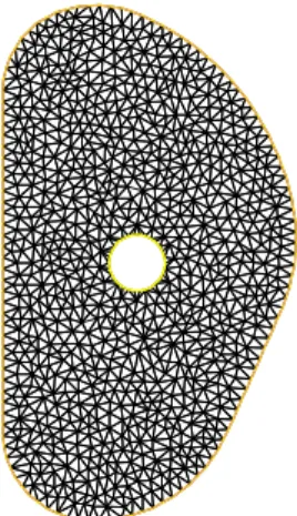
All the numerical results presented in the remaining part of this paper were obtained using the software FreeFem++ (http ://www.freefem.org/ff++/). We are concerned with the geometry of ITER and the mesh used for the computations is shown on Fig. 3. It is composed of 1804 triangles and 977 nodes 150 of which are boundary nodes divided into 120 nodes onΓV and 30= NΓI onΓI. The shape ofΓI is chosen empirically.

3.2. Twin experiments

Numerical experiments with simulated input Cauchy data are conducted in order to validate the algorithm. Assume we are provided with a Neumann boundary condition function g onΓV. We generate the associated Dirichlet function f onΓV assuming a

reference Dirichlet function uref is known onΓI. We thus solve the following boundary

value problem :            LψN,ref(uref, g) = 0 in Ω 1 r∂nψN,ref(uref, g) = g on ΓV ψN,ref(uref, g) = uref on ΓI

(37)

and set f = ψN,ref(uref, g)|ΓV.

We have considered two test cases. In the first one (TC1)

uref(r, z) = 50 sin(r)2+ 50 on ΓI (38)

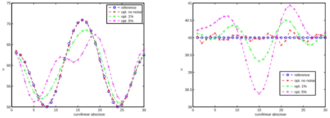
and in the second one (TC2) uref is simply a constant

uref(r, z) = 40 on ΓI (39)

The numerical experiments consist in minimizing the regularized error functional Jε

defined thanks to f and g. The obtained optimal solution uoptand the associated ψopt

are then compared to uref and ψref which should ideally be recovered. Three cases are

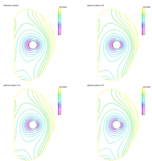
considered : the noise free case, a1% noise on f and g and a 5% noise.

When the noise on f and g is small and the recovery of u is excellent there is very little difference between the Dirichlet solution ψD(uopt, f) and the Neumann solution ψN(uopt, g). However this is not the case any longer when the level of noise increases.

The Dirichlet solution is much more sensitive to noise on f than the Neumann solution is sensitive to noise on g. Therefore the optimal solution is chosen to be ψopt= ψN(uopt, g).

The results are shown on Figs. 4 and 5 where the reference and recovered solutions are shown for the three levels of noise considered. The results are excellent for the noise free case in which the Dirichlet boundary condition u is almost perfecty recovered (Fig. 6). The differences between uoptand uref increase with the level of noise (Fig. 6 and Tab.

1). As it is often the case in this type of inverse problems the most important errors on

ψoptare localized close to the boundaryΓI and vanishes as we move away from it (Fig.

7).

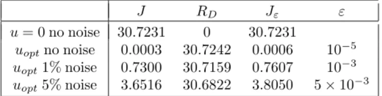
Tables 2 and 3 sumarize the evolution of the values of J , RDand Jεfor the different

IsoValue 16 20 22 25 27 29 31 35 39 42 44 47 50 53 56 58 61 64 67 69 reference solution IsoValue 16 20 22 25 27 29 31 35 39 42 44 47 50 53 56 58 61 64 67 69 optimal solution 0% IsoValue 16 20 22 25 27 29 31 35 39 42 44 47 50 53 56 58 61 64 67 69 optimal solution 1% IsoValue 16 20 22 25 27 29 31 35 39 42 44 47 50 53 56 58 61 64 67 69 optimal solution 5%

Figure 4. First test case (TC1), uref given by Eq. (38). Top left : reference solution

ψN,ref(uref, g). Top right : recovered solution with no noise on the data. Bottom left :

recovered solution with a1%noise on the data. Bottom right : recovered solution with a

5%noise.

that the regularization parameter was chosen differently from one experiment to another depending on the noise level. This was tuned by hand. In the next section we propose to use the L-curve method [19] to choose the value of ε.

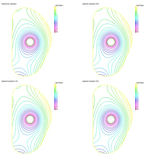
IsoValue -2 0 2 5 7 9 11 13 16 18 20 22 24 26 28 31 33 35 37 39 reference solution IsoValue -2 0 2 5 7 9 11 13 16 18 20 22 24 26 28 31 33 35 37 39 optimal solution 0% IsoValue -2 0 2 5 7 9 11 13 16 18 20 22 24 26 28 31 33 35 37 39 optimal solution 1% IsoValue -2 0 2 5 7 9 11 13 16 18 20 22 24 26 28 31 33 35 37 39 optimal solution 5%

Figure 5. Second test case (TC2),uref given by Eq. (39). Top left : reference solution

ψN,ref(uref, g). Top right : recovered solution with no noise on the data. Bottom left :

recovered solution with a1%noise on the data. Bottom right : recovered solution with a

0 5 10 15 20 25 30 50 55 60 65 70 75 curvilinear abscisse u reference opt. no noise opt. 1% opt. 5% 0 5 10 15 20 25 30 38 38.5 39 39.5 40 40.5 41 curvilinear abscisse u reference opt. no noise opt. 1% opt. 5%

Figure 6.uref and the recovereduopt for the 3 levels of noise on the data. Left : TC1.

Right TC2. IsoValue 0.00381985 0.0114501 0.0190803 0.0267105 0.0343407 0.0419709 0.0496011 0.0572313 0.0648615 0.0724917 0.080122 0.0877522 0.0953824 0.103013 0.110643 0.118273 0.125903 0.133533 0.141164 0.148794 relative error

noise level error TC1 error TC2

0% 0.0131 0.0055 1% 0.0659 0.0170 5% 0.1526 0.0405

Tableau 1. Maximum relative error|uopt− uref| |uref| for TC 1 and 2 . J RD Jε ε u= 0 no noise 46.8643 0 46.8643 uoptno noise 0.0021 46.8722 0.0026 10−5 uopt1% noise 1.8443 46.5553 1.8676 5 × 10−4 uopt5% noise 9.2180 46.5575 9.2646 10−3

Tableau 2. TC1 results. Values of the error functional, the regularization term, the total

cost function and the chosen regularization parameter for the initial guess (row 1), the optimal solutions for different noise levels (row 2, 3 and 4).

J RD Jε ε u= 0 no noise 30.7231 0 30.7231

uoptno noise 0.0003 30.7242 0.0006 10−5 uopt1% noise 0.7300 30.7159 0.7607 10−3 uopt5% noise 3.6516 30.6822 3.8050 5 × 10−3

Tableau 3. TC2 results. Values of the error functional, the regularization term, the total

cost function and the chosen regularization parameter for the initial guess (row 1), the optimal solutions for different noise levels (row 2, 3 and 4).

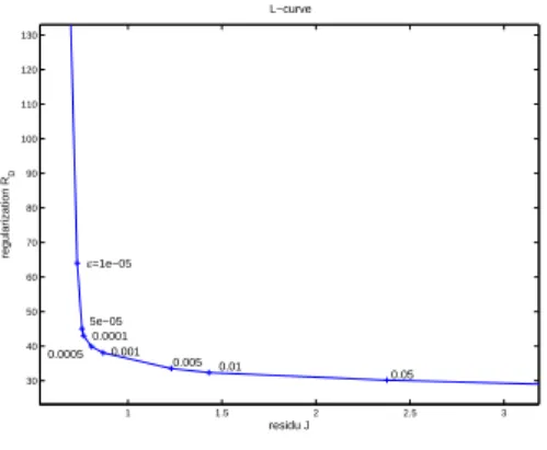
1 1.5 2 2.5 3 30 40 50 60 70 80 90 100 110 120 130 residu J regularization R D ε=1e−05 5e−05 0.0001 0.0005 0.001 0.005 0.01 0.05 L−curve

Figure 8. L-curve computed for the ITER case. The corner is located atε = 5 × 10−4_.

3.3. An ITER equilibrium

In this last numerical experiment we consider a ’real’ ITER case. Measurements of the magnetic field are provided by the plasma equilibrium code CEDRES++ [17]. These mesurements are interpolated to provide f and g onΓV. The regularized error functional

is then minimized to compute the optimal uopt. The choice of the regularization

parame-ter ε is made thanks to the computation of the L-curve shown on Fig. 8. It is a plot of

(J(uopt)(ε), RD(uopt)(ε)) as ε varies. The corner of the L-shaped curve provides a value

of ε= 5.10−4_.

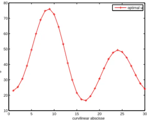
The computed uoptis shown on Fig. 9 and numerical values are given in Tab. 4. The

recovered poloidal flux ψ is shown on Fig. 10. The boundary of the plasma is found to be the isoflux ψ= 16.3 which shows an X-point configuration.

J RD Jε ε u= 0 31.1026 0 31.1026

uopt 0.8053 39.9169 0.8253 5 × 10−4

Tableau 4. ITER case results. Values of the error functional, the regularization term, the

total cost function and the chosen regularization parameter for the initial guess (row 1) and the optimal solution (row 2)

0 5 10 15 20 25 30 10 20 30 40 50 60 70 80 curvilinear abscisse u optimal u

Figure 9. Optimaluoptfor the ITER case.

IsoValue 0 2 4 6 8 10 12 13 14 15 16 16.3 17 18 19 20 21 22 23 24 26 28 30 32 34 36 38 40 42 50 optimal solution

4. Conclusion

We have presented a numerical method for the computation of the poloidal flux in the vacuum region surrounding the plasma in a Tokamak. The algorithm is based on the optimization of a regularized error functional. This computation enables in a second step the identification of the plasma boundary.

Numerical experiments have been conducted. They show that the method is precise and robust to noise on the Cauchy input data. It is fast since the optimization reduces to the resolution of a linear system of very reasonable dimension. Successive equilibrium reconstructions can be conducted very rapidly since the matrix of this linear system can be completely precomputed and only the right hand side has to be updated. The L-curve method proved to be efficient to specify the regularization parameter.

Appendix. Proof of Proposition 1

1. We need to prove the continuity and the coercivity of Jε.

Continuity.

The maps v 7→ ψD(v) and v 7→ ψN(v) are continuous and linear from H1/2(ΓI) to H1_{(Ω). Moreover since ˜ψ}

D(f ) and ˜ψN(g) are in H1(Ω) and rM ≥ r ≥ rm>0 in Ω it

is shown with Cauchy Schwarz that the bilinear forms sDand sN, the linear form l and

thus Jεare continuous on H1/2(ΓI).

Coercivity.

The bilinear form sDis coercive on H1/2(ΓI). One obtains this from the fact that ψD(v) ∈ H1

0(Ω, ΓV) and the Poincaré inequality holds, and from the continuity of the application ψD(v) ∈ H1(Ω) → ψD(v)|ΓI = v ∈ H

1/2_(Γ I).

On the contrary, since for ψN(v) ∈ H1(Ω) the seminorm does not bound the L2norm,

the bilinear form sN is not coercive and because of the minus sign in s= sD− sN we

need to prove that s(v, v) ≥ 0 to obtain the coercivity of the bilinear part of functional Jε. One can use the same type of argument as in [5] to de so.

Eventually it holds that

1 2s(v, v) + ε 2sD(v, v) ≥ Cε||v|| 2 H1/2(ΓI)

Using the continuity and the coercivity of Jεit results from [25] that problem Pεadmits

a unique solution uε∈ U.

The solution uεis characterized by the first order optimality condition which is written

as the following well-posed variational problem

(Jε′(uε), v) = εsD(uε, v) + sD(uε, v) − sN(uε, v) − l(v) = 0 ∀v ∈ U (40)

which as in Eq. (26) can be understood as an equality onΓI.

2. The stability result is deduced from the optimality condition (40).

Let u1_ε(resp. u2_ε) be the solution associated to(f1_{, g}1_{) (resp. (f}2_{, g}2_{)). Substracting}

the two optimality conditions, choosing v= u1

ε− u2εand using the coercivity leads to Cε||u1ε− u2ε||2H1/2(ΓI)≤ |(l1− l2)(u

1 ε− u2ε)|

The map f 7→ ˜ψD(f ) is linear and continuous from H1/2(ΓV) to H1(Ω), and so is the

map g 7→ ˜ψN(g) from H−1/2(ΓV) to H1(Ω). Using these facts and Cauchy Schwarz it

follows that ||u1ε− u2ε||H1/2_(ΓI)≤ C′ rmC 1 ε(||f 1_{− f}2_|| H1/2_(ΓV)+ ||g1− g2||_H−1/2_(ΓV))

3. For this point the proof of Proposition3.2 in [3] can be adpated. A sketch of the

proof is as follows. Let us suppose that there exists u∈ U such that ψD(u, f ) = ψN(u, g).

A key point is to show that sD(uε, uε) → sD(u, u) when ε → 0. Then in a second step

using the optimality conditions for u and uεit is shown that sD(uε− u, uε− u) ≤ sD(u, u) − sD(uε, uε)

5. Bibliographie

[1] S. Andrieux, T.N. Baranger, and A. Ben Abda. Solving cauchy problems by minimizing an energy-like functional. Inverse Problems, 22 :115–133, 2006.

[2] S. Andrieux, A. Ben Abda, and T.N. Baranger. Data completion via an energy error functional.

C.R. Mecanique, 333 :171–177, 2005.

[3] M. Azaiez, F. Ben Belgacem, and H. El Fekih. On Cauchy’s problem : II. Completion, regula-rization and approximation. Inverse Problems, 22 :1307–1336, 2006.

[4] A Ben Abda, M. Hassine, M. Jaoua, and M. Masmoudi. Topological sensitivity analysis for the location of small cavities in stokes flows. SIAM J. Cont. Opt., 2009.

[5] F. Ben Belgacem and H. El Fekih. On Cauchy’s problem : I. A variational Steklov-Poincaré theory. Inverse Problems, 21 :1915–1936, 2005.

[6] J. Blum. Numerical Simulation and Optimal Control in Plasma Physics with Applications to

Tokamaks. Series in Modern Applied Mathematics. Wiley Gauthier-Villars, Paris, 1989.

[7] M. Bonnet and A. Constantinescu. Inverse problems in elasticity. Inverse Problems, 21(2), 2005.

[8] L. Bourgeois and J. Dardé. A quasi-reversibility approach to solve the inverse obstacle pro-blem. Inverse Problems and Imaging, 4/3 :351–377, 2010.

[9] B.J. Braams. The interpretation of tokamak magnetic diagnostics. Nuc. Fus., 33(7) :715–748, 1991.

[10] S. Chaabane and M. Jaoua. Identification of robin coefficients by means of boundary measu-rements. Inverse Problems, 15(6) :1425, 1999.

[11] P.G. Ciarlet. The Finite Element Method For Elliptic Problems. North-Holland, 1980. [12] R. Courant and D. Hilbert. Methods of Mathematical Physics, volume 1-2. Interscience,

1962.

[13] W. Feneberg, K. Lackner, and P. Martin. Fast control of the plasma surface. Computer

Physics Communications, 31(2) :143–148, 1984.

[14] Y. Fischer. Approximation dans des classes de fonctions analytiques généralisées et

résolu-tion de problèmes inverses pour les tokamaks. Phd thesis, Université de Nice Sophia Antipolis,

France, 2011.

[15] Y. Fischer, B. Marteau, and Y. Privat. Some inverse problems around the tokamak tore supra.

Comm. Pure and Applied Analysis, to appear.

[16] H. Grad and H. Rubin. Hydromagnetic equilibria and force-free fields. In 2nd U.N.

Confe-rence on the Peaceful uses of Atomic Energy, volume 31, pages 190–197, Geneva, 1958.

[17] V. Grandgirard. Modélisation de l’équilibre d’un plasma de tokamak - Tokamak plasma

[18] H. Haddar and R. Kress. Conformal mappings and inverse boundary value problem. Inverse

Problems, 21 :935–953, 2005.

[19] C. Hansen. Rank-Deficient and Discrete Ill-Posed Problems : Numerical Aspects of Linear

Inversion. SIAM, Philadelphia, 1998.

[20] R.V. Kohn and A. McKenney. Numerical implementation of a variational method for electri-cal impedance tomography. Inverse Problems, 6(3) :389, 1990.

[21] R.V. Kohn and M.S. Vogelius. Determining conductivity by boundary measurements : II. Interior results. Commun. Pure Appl. Math., 31 :643–667, 1985.

[22] R.V. Kohn and M.S. Vogelius. Relaxation of a variational method for impedance computed tomography. Commun. Pure Appl. Math., 11 :745–777, 1987.

[23] K. Lackner. Computation of ideal MHD equilibria. Computer Physics Communications, 12 :33–44, 1976.

[24] P. Ladeveze and D. Leguillon. Error estimate procedure in the finite element method and applications. SIAM J. Num. Anal., 20(3) :485–509, 1983.

[25] J.L. Lions. Contrôle optimal de systèmes gouvernés par des équations aux dérivées partielles

(Optimal control of systems governed by partial differential equations). Dunod, Paris, 1968.

[26] D.P. O’Brien, J.J Ellis, and J. Lingertat. Local expansion method for fast plasma boundary identification in JET. Nuc. Fus., 33(3) :467–474, 1993.

[27] A. Quarteroni and V Alberto. Domain Decomposition Methods for Partial Differential

Equa-tions. Oxford University Press, 1999.

[28] F. Saint-Laurent and G. Martin. Real time determination and control of the plasma localisa-tion and internal inductance in Tore Supra. Fusion Engineering and Design, 56-57 :761–765, 2001.

[29] F. Sartori, A. Cenedese, and F. Milani. JET real-time object-oriented code for plasma boun-dary reconstruction. Fus. Engin. Des., 66-68 :735–739, 2003.

[30] V.D. Shafranov. On magnetohydrodynamical equilibrium configurations. Soviet Physics

JETP, 6(3) :1013, 1958.

[31] V.D. Shafranov and L.E. Zakharov. Use of the virtual-casing principle in calculating the containing magnetic field in toroidal plasma systems. Nuc. Fus., 12 :599–601, 1972.

[32] J. Wesson. Tokamaks, volume 118 of International Series of Monographs on Physics. Oxford University Press Inc., New York, Third Edition, 2004.