Modelling and flexible predictive control of building space-heating demand in district heating systems

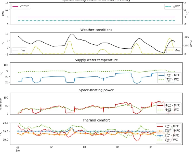
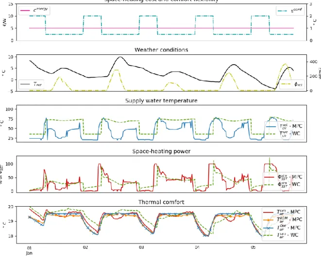
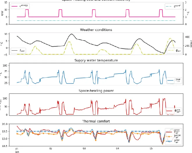
If we look at the thermal comfort, it is clear that the two predictive controllers give very interesting results because the in- door operative temperature is maintained in the

مﺎﳋا ﻲﻠﶈا ﺞﺗﺎﻨﻟا ﰲ عﺎﻄﻘﻟا ﺔﳘﺎﺴﻣ ﺎﻣأ 8 (PIB ) ﺎﲟ ﺔﻴﺣﺎﻴﺴﻟا تاداﺮﻳﻹا ﰲ ةدﺎﻳﺰﻟا رﻮﻄﺗ لﺪﻌﲟ ﺖﻧﺎﻜﻓ برﺎﻘﻳ 7 ﱃإ 9 ﺔﻨﺴﺑ ﺔﻧرﺎﻘﻣ فﺎﻌﺿأ تاﺮﻣ 2007 عﺎﻄﻗ ﺎﻫﺮﻓﻮﻳ ﱵﻟا

Unite´ de recherche INRIA Lorraine, Technoˆpole de Nancy-Brabois, Campus scientifique, 615 rue de Jardin Botanique, BP 101, 54600 VILLERS LE`S NANCY Unite´ de recherche INRIA

The spectacular growth of Río Bec style construction in Group C since Makan 2, its parallel evolution with Group B during the Terminal Classic period and their spatial proximity

Differences between direct and reversed polarity treatment administration indicated that FEAST is clearly initiating seizure activity in the frontal region (right 4 left).

In this study, data collected on the passive seismic network have been used to further understand the reservoir by: 1) locating hypocenters to identify active faults / fractures in

Private Membership Query using PBR. This protocol essentially follows the same prin- ciple as the one which combines PIR and a Bloom filter. Again k PBR invocations are required

Celui qui se prévaut d'un contrat de travail doit apporter la preuve de 11nexac- titude de la qualification de contrat d'entreprise par l'apport d'éléments

References

[1] CEREMA, Chiffres-cles sur la consommation énergétique dans les bâtiments, (2013). http://reseaux-chaleur.cerema.fr/consommation-denergie-dans-les-batiments-chiffres-cles-2013.
[2] ADEME, Chiffres-clés sur le climat, air et energie, (2014). https://www.ademe.fr/sites/default/files/assets/documents/chiffres-cles-climat-air-energie-8705-bd.pdf.
[3] H. Lund, B. Möller, B.V. Mathiesen, A. Dyrelund, The role of district heating in future renewable energy systems, Energy. 35 (2010) 1381–1390. doi:10.1016/j.energy.2009.11.023.
[4] M. Münster, P.E. Morthorst, H.V. Larsen, L. Bregnbæk, J. Werling, H.H. Lindboe, H. Ravn, The role of district heating in the future Danish energy system, Energy. 48 (2012) 47–55. doi:10.1016/j.energy.2012.06.011.
[5] H. Lund, S. Werner, R. Wiltshire, S. Svendsen, J.E. Thorsen, F. Hvelplund, B.V. Mathiesen, 4th Generation District Heating (4GDH), Energy. 68 (2014) 1–11. doi:10.1016/j.energy.2014.02.089. [6] S. Werner, District heating and cooling in Sweden, Energy. 126 (2017) 419–429.
doi:10.1016/j.energy.2017.03.052.
[7] H. Lund, N. Duic, P.A. Østergaard, B.V. Mathiesen, Future district heating systems and technologies: On the role of smart energy systems and 4th generation district heating, Energy. 165 (2018) 614–619. doi:10.1016/j.energy.2018.09.115.
[8] S. Fazlollahi, N. Schüler, F. Maréchal, A solid thermal storage model for the optimization of buildings operation strategy, Energy. 88 (2015) 209–222. doi:10.1016/j.energy.2015.04.085. [9] E. Guelpa, G. Barbero, A. Sciacovelli, V. Verda, Peak-shaving in district heating systems through
optimal management of the thermal request of buildings, Energy. (2017). doi:10.1016/j.energy.2017.06.107.
[10] D.F. Dominković, P. Gianniou, M. Münster, A. Heller, C. Rode, Utilizing thermal building mass for storage in district heating systems: Combined building level simulations and system level optimization, Energy. 153 (2018) 949–966. doi:10.1016/j.energy.2018.04.093.
[11] P.-D. Moroşan, R. Bourdais, D. Dumur, J. Buisson, Building temperature regulation using a distributed model predictive control, Energy Build. 42 (2010) 1445–1452. doi:10.1016/j.enbuild.2010.03.014.
[12] F. Oldewurtel, A. Parisio, C.N. Jones, D. Gyalistras, M. Gwerder, V. Stauch, B. Lehmann, M. Morari, Use of model predictive control and weather forecasts for energy efficient building climate control, Energy Build. 45 (2012) 15–27. doi:10.1016/j.enbuild.2011.09.022.
[13] M.Y. Lamoudi, Distributed model predictive control for energy management in building, PhD Thesis, Université Grenoble Alpes, 2012. https://tel.archives-ouvertes.fr/tel-00875593/document (accessed January 18, 2017).
[14] D. Sturzenegger, D. Gyalistras, M. Morari, R.S. Smith, Model Predictive Climate Control of a Swiss Office Building: Implementation, Results, and Cost–Benefit Analysis, IEEE Trans. Control Syst. Technol. 24 (2016) 1–12. doi:10.1109/TCST.2015.2415411.
(33)
1 2 3 4 5 6 7 8 9 10 11 12 13 14 15 16 17 18 19 20 21 22 23 24 25 26 27 28 29 30 31 32 33 34 35 36 37 38 39 40 41 42 43 44 45 46 47 48 49 50 51 52 53 54 55 56 57 58 59 60 61
[15] R. De Coninck, L. Helsen, Practical implementation and evaluation of model predictive control for an office building in Brussels, Energy Build. 111 (2016) 290–298. doi:10.1016/j.enbuild.2015.11.014.
[16] S. Prívara, J. Široký, L. Ferkl, J. Cigler, Model predictive control of a building heating system: The first experience, Energy Build. 43 (2011) 564–572. doi:10.1016/j.enbuild.2010.10.022.
[17] F. Verrilli, S. Srinivasan, G. Gambino, M. Canelli, M. Himanka, V. Del, M. Sasso, L. Glielmo, Model Predictive Control-based optimal operations of district heating system with thermal energy storage and flexible loads, (2016). doi:10.1109/TASE.2016.2618948.
[18] M. Killian, M. Kozek, Ten questions concerning model predictive control for energy efficient buildings, Build. Environ. 105 (2016) 403–412. doi:10.1016/j.buildenv.2016.05.034.
[19] S. Prívara, J. Cigler, Z. Váňa, F. Oldewurtel, C. Sagerschnig, E. Žáčeková, Building modeling as a crucial part for building predictive control, Energy Build. 56 (2013) 8–22. doi:10.1016/j.enbuild.2012.10.024.
[20] A. Foucquier, S. Robert, F. Suard, L. Stéphan, A. Jay, State of the art in building modelling and energy performances prediction: A review, Renew. Sustain. Energy Rev. 23 (2013) 272–288. doi:10.1016/j.rser.2013.03.004.
[21] S. Prívara, Z. Váňa, E. Žáčeková, J. Cigler, Building modeling: Selection of the most appropriate model for predictive control, Energy Build. 55 (2012) 341–350. doi:10.1016/j.enbuild.2012.08.040.
[22] M. Wetter, W. Zuo, T.S. Nouidui, Modeling of heat transfer in rooms in the modelica “buildings” library, in: Proc. Build. Simul. 2011 12th Conf. Int. Build. Perform. Simul. Assoc., 2011: pp. 1096– 1103. https://miami.pure.elsevier.com/en/publications/modeling-of-heat-transfer-in-rooms-in-the-modelica-buildings-libr (accessed January 21, 2019).
[23] J. Le Dréau, P. Heiselberg, Energy flexibility of residential buildings using short term heat storage in the thermal mass, Energy. 111 (2016) 991–1002. doi:10.1016/j.energy.2016.05.076. [24] H. Wolisz, T.M. Kull, R. Streblow, D. Müller, The effect of furniture and floor covering upon
dynamic thermal building simulations, in: 2015: pp. 2154–2159. doi:10.1016/j.egypro.2015.11.304.
[25] K.A. Antonopoulos, E.P. Koronaki, Effect of indoor mass on the time constant and thermal delay of buildings, Int. J. Energy Res. 24 (2000) 391–402. doi:10.1002/(SICI)1099-114X(200004)24:5<391::AID-ER585>3.0.CO;2-L.
[26] H. Johra, P. Heiselberg, Influence of internal thermal mass on the indoor thermal dynamics and integration of phase change materials in furniture for building energy storage: A review, Renew. Sustain. Energy Rev. 69 (2017) 19–32. doi:10.1016/j.rser.2016.11.145.
[27] N. Aoun, R. Bavière, M. Vallée, A. Brun, G. Sandou, Dynamic simulation of residential buildings supporting the development of flexible control in district heating systems, in: 13th Int. Model. Conf., Regensburg, Germany, 2019.
[28] City-zen, City-zen Project, Cityzen-Smartcity. (2018). http://www.cityzen-smartcity.eu/.
[29] J. Vivian, A. Zarrella, G. Emmi, M. De Carli, An evaluation of the suitability of lumped-capacitance models in calculating energy needs and thermal behaviour of buildings, Energy Build. 150 (2017) 447–465. doi:10.1016/j.enbuild.2017.06.021.
(34)
[30] T. Berthou, P. Stabat, R. Salvazet, D. Marchio, Development and validation of a gray box model to predict thermal behavior of occupied office buildings, Energy Build. 74 (2014) 91–100. doi:10.1016/j.enbuild.2014.01.038.
[31] H. Harb, N. Boyanov, L. Hernandez, R. Streblow, D. Müller, Development and validation of grey-box models for forecasting the thermal response of occupied buildings, Energy Build. 117 (2016) 199–207. doi:10.1016/j.enbuild.2016.02.021.
[32] P. Bacher, H. Madsen, Identifying suitable models for the heat dynamics of buildings, Energy Build. 43 (2011) 1511–1522. doi:10.1016/j.enbuild.2011.02.005.
[33] M. Wetter, GenOpt (R), Generic Optimization Program, User Manual, Version 3.1.1, Lawrence Berkeley National Laboratory: Berkeley, CA, USA, 2016. http://simulationresearch.lbl.gov/GO/. [34] N. Aoun, R. Bavière, M. Vallée, G. Sandou, Development and assessment of a reduced-order
building model designed for model predictive control of space-heating demand in district heating systems, in: Wroclaw, Poland, 2019.
[35] L. Giraud, M. Merabet, R. Baviere, M. Vallée, Optimal control of district heating systems using dynamic simulation and mixed integer linear programming, in: Proc. 12th Int. Model. Conf. Prague Czech Repub. May 15-17 2017, Linköping University Electronic Press, 2017: pp. 141– 150.
[36] Q. Wu, H. Ren, W. Gao, J. Ren, Multi-objective optimization of a distributed energy network integrated with heating interchange, Energy. 109 (2016) 353–364.
[37] M. Leśko, W. Bujalski, K. Futyma, Operational optimization in district heating systems with the use of thermal energy storage, Energy. 165 (2018) 902–915. doi:10.1016/j.energy.2018.09.141. [38] S. Fazlollahi, N. Schüler, F. Maréchal, A solid thermal storage model for the optimization of
buildings operation strategy, Energy. 88 (2015) 209–222. doi:10.1016/j.energy.2015.04.085. [39] M.J. Risbeck, C.T. Maravelias, J.B. Rawlings, R.D. Turney, A mixed-integer linear programming
model for real-time cost optimization of building heating, ventilation, and air conditioning equipment, Energy Build. 142 (2017) 220–235.
[40] V. Kumtepeli, Y. Zhao, M. Naumann, A. Tripathi, Y. Wang, A. Jossen, H. Hesse, Design and analysis of an aging-aware energy management system for islanded grids using mixed-integer quadratic programming, Int. J. Energy Res. (2019).
[41] M. Killian, M. Zauner, M. Kozek, Comprehensive smart home energy management system using mixed-integer quadratic-programming, Appl. Energy. 222 (2018) 662–672.
[42] P. Vögelin, B. Koch, G. Georges, K. Boulouchos, Heuristic approach for the economic optimisation of combined heat and power (CHP) plants: Operating strategy, heat storage and power, Energy. 121 (2017) 66–77. doi:https://doi.org/10.1016/j.energy.2016.12.133.
[43] M. Vallée, R. Bavière, V. Seguin, V. Vuillerme, N. Lamaison, M. Descamps, A. Aurousseau, An efficient co-simulation and control approach to tackle complex multi-domain energetic systems: concepts and applications of the PEGASE tool, in: Wroclaw, Poland, 2019.
[44] FMI interface, Httpsfmi-Stand. (2019).
[45] G.P. McCormick, Computability of global solutions to factorable nonconvex programs: Part I— Convex underestimating problems, Math. Program. 10 (1976) 147–175.
Figure
Figure 1. Schematic representation of a floor discretized into 4 equivalent thermal zones and the modelled thermal  phenomena in the building simulator
Figure 3. Photograph of the advanced control strategies demonstrator Le Salammbô – Grenoble, 2018   Photo credit: http://www.gre-mag.fr
Figure 4. RC representation of the building model structure