HAL Id: hal-01274200
https://hal.inria.fr/hal-01274200
Submitted on 15 Feb 2016
HAL is a multi-disciplinary open access
archive for the deposit and dissemination of
sci-entific research documents, whether they are
pub-lished or not. The documents may come from
teaching and research institutions in France or
abroad, or from public or private research centers.
L’archive ouverte pluridisciplinaire HAL, est
destinée au dépôt et à la diffusion de documents
scientifiques de niveau recherche, publiés ou non,
émanant des établissements d’enseignement et de
recherche français ou étrangers, des laboratoires
publics ou privés.
Using Finite Forkable DEVS for Decision-Making Based
on Time Measured with Uncertainty
Damián Vicino, Olivier Dalle, Gabriel Wainer
To cite this version:
Damián Vicino, Olivier Dalle, Gabriel Wainer. Using Finite Forkable DEVS for Decision-Making
Based on Time Measured with Uncertainty. Eighth EAI International Conference on Simulation Tools
and Techniques (SIMUTOOLS 2015), Aug 2015, Athènes, Greece. �10.4108/eai.24-8-2015.2261152�.
�hal-01274200�
Using Finite Forkable DEVS for Decision-Making Based on
Time Measured with Uncertainty
Damián Vicino
∗ † ‡Université Nice Sophia Antipolis I3S UMR CNRS 7271 INRIA - Sophia Antipolis
Carleton University Dept. of Systems and Computer Engineering
[email protected]
Olivier Dalle
∗ †Université Nice Sophia Antipolis I3S UMR CNRS 7271 INRIA - Sophia Antipolis
[email protected]
Gabriel Wainer
‡Carleton University Dept. of Systems and Computer Engineering
[email protected]
ABSTRACT
The time-line in Discrete Event Simulation (DES) is a se-quence of events defined in a numerable subset of R+. When
it comes from an experimental measurement, the timing of these events has a limited precision. This precision is usually well-known and documented for each instruments and pro-cedures used for collecting experimental datas. Therefore, these instruments and procedures produce measurement re-sults expressed using values each associated with an uncer-tainty quantification, given by unceruncer-tainty intervals. Tools have been developed in Continuous Systems modeling for deriving the uncertainty intervals of the final results cor-responding to the propagation of the uncertainty intervals being evaluated. These tools cannot be used in DES as they are defined, and no alternative tools that would apply to DES have been developed yet. In this paper, we propose simulation algorithms, based on the Discrete Event System Specification (DEVS) formalism, that can be used to sim-ulate and obtain every possible output and state trajecto-ries of simulations that receive input values with uncertainty quantification. Then, we present a subclass of DEVS mod-els, called Finite Forkable DEVS (FF-DEVS), that can be simulated by the proposed algorithms. This subclass en-sures that the simulation is forking only a finite number of processes for each simulation step. Finally, we discuss the ∗Université Nice Sophia Antipolis, Laboratoire I3S UMR CNRS 7271, 2000 route des Lucioles, BP 93, 06900 Sophia Antipolis, France
†INRIA - Sophia Antipolis, 2004 Route des Lucioles, 06903 Sophia Antipolis, France
‡Carleton University, Dept. of Systems and Com-puter Engineering, 1125 Colonel By Dr., Ottawa, ON, Canada
simulation of a traffic light model and show the trajectories obtained when it is subject to input uncertainty.
Categories and Subject Descriptors
I.6.8 [Types of Simulation]: Discrete event; I.1.2 [Symbolic and algebraic manipulation]: Algorithms; F.2.2 [Analysis of algorithms and problem complexity]: Nonnumerical Algorithms and Problems—Sequencing and scheduling
General Terms
Theory, Algorithms
Keywords
DEVS, uncertainty, metrology, time interval
1.
INTRODUCTION
Discrete-event simulation (DES) is a technique in which the simulation engine plays a history following a chronology of events. The technique is called ”discrete-event” because the processing of each event of the chronology takes place at discrete points of a continuous time-line and takes no time with respect to the virtual simulated time (even though it may take a non-negligible time to compute with respect to the real wall-clock time).
One of many usages of DES is being part of a decision-making process for industrial and research works. Here, data is collected from the real system using metrological in-struments and processes. From them, a set of measurement results is obtained and used as input to feed the simulation. Modern metrology processes [3] state that it is not possible to determine a unique true value for a measurand and all measurement results require a quantification of its uncer-tainty to be complete.
The Bureau International des Poids et Mesures (BIPM) de-fines in [3] the proper procedures to obtain measurement re-sults and the basic concepts behind them. The measurement result with uncertainty quantification is usually represented as an uncertainty interval with a certain level of confidence associated. We will not enter in the details of how the
mea-surement result is obtained in this paper, but rather in how to use it for simulation.
In the context of DES, we consider the result of a simula-tion to be a trajectory of states or outputs describing the dynamic behavior of the model. In DES a small change in the timing of an event may produce a different state or out-put. Having uncertainty about the time of the input events may produce a tree-like result (with uncertainty time com-ponent) in place of a linear sequence of states.
As far as we know, no work has been done in DES to obtain all possible trajectories using a set of measured events as inputs and considering their timing uncertainty quantifica-tion.
We have special interest in the set of DES models described by the Discrete Event System Specification (DEVS) for-malisms family and reusing previously defined models. We set our goal to provide the means to obtain all the possible state and output trajectories (as a tree) for DEVS models. Our scientific contribution here are the abstract algorithms to simulate DEVS models with input events having uncer-tainty quantification of the time component. We provide the characterization of a subclass of DEVS models that can be simulated forking finite processes in each simulation step by the previously mentioned algorithms, the Finite Forkable DEVS (FF-DEVS).
We describe the limitations of the FF-DEVS subclass and show examples of DEVS models that are part or not of this subclass. We compare FF-DEVS against other subclasses defined in the literature.
We end our presentation of FF-DEVS with a case study showing the application of the algorithms simulating a traffic-light with a pedestrian call button. We present the trajec-tories obtained based on different input values and accuracy levels and discuss the potential of this method.
2.
BACKGROUND
2.1
Discrete-Event System Specification (DEVS)
Among the many Discrete-Event Simulation techniques, our focus is on the DEVS formalism [19, 18], which provides a theoretical framework to think about Modeling using a hi-erarchical, modular approach. The modeling hierarchy has two kinds of components: atomic models and coupled mod-els.
In DEVS two kinds of events are supported:
• Exogenous events: occurrence of an input at a given simulation time.
• Endogenous events: occurrence of an internal transi-tion after having no exogenous events for a given sim-ulation time.
The abstract simulator for DEVS defined in [ZPK+76, ZPK00] is divided in three components named simulator (for atomic models), coordinator (for coupled models) and root-coordinator for the main loop of the simulation.
Multiple extensions had being defined for this formalism in the past few decades. We find particularly relevant for our work the subclasses Schedule Preserved DEVS (SP-DEVS) [9] and Finite & Deterministic DEVS (FD-DEVS) [10].
Both extensions, SP-DEVS and FD-DEVS, subclass DEVS for researching state reachability. In some sense, our prob-lem can be thought as finding state reachability bounded to time intervals and a selection of messages.
The FD-DEVS subclass is restricted to those models having a finite set of states and scheduling transitions expressed by rational time advances.
The SP-DEVS subclass, which subclasses FD-DEVS, is re-stricted to the models that do not change scheduled transi-tion times when receiving an exogenous event.
2.2
Metrology
For the metrology concepts and terminology used in this pa-per, we follow Guide to expression of Uncertainty in Mea-surement [3] and International Vocabulary of Metrology [4] documents provided by Bureau International de Poids et Mesures (BIPM).
Mostly, we only make reference to three metrological terms: • Measurand [4]: “quantity intended to be measured”. • Measurement Result [4]: “set of quantity values
be-ing attributed to a measurand together with any other available relevant information”, “Note 2: A measure-ment result is generally expressed as a single measured quantity value and a measurement uncertainty”. • Measurement Uncertainty [4, 3]: “non-negative
param-eter characterizing the dispersion of the quantity val-ues being attributed to a measurand, based on the in-formation used”.
2.3
Interval Arithmetic
The measurement results can be described as intervals of real numbers. A way to properly work with them is using interval arithmetic, which describes how to operate with this kind of data [16].
In interval arithmetic, the addition of two intervals is de-fined as the interval where lower endpoint is dede-fined by the addition of the two lower endpoints and higher endpoint is defined by the addition of the two higher endpoints. Similar definitions exist for other operations as subtraction, multi-plication and division.
The definition of comparison operations for intervals is more complicated because the two intervals being compared may intersect, which results in multiple comparison cases that require proper handling[1, 16].
To reduce the amount of notation being introduced, we ex-press the few comparisons between intervals used for the presented algorithms using comparison on their endpoint values.
3.
RELATED WORK
The closer match to our work are studies on state reachabil-ity tools and properties.
In [8], state reachability is studied for a subset of DEVS models having a finite set of states. An algorithm is provided to decide if a state is reachable or not when simulating a model.
In [10], Finite & Deterministic DEVS is formally defined and algorithms to study of all reachable state based in graph theory are provided.
In [9], Scheduling Preserved DEVS is introduced as a sub-class of FD-DEVS. A timed language is also introduced that allows characterization of reachable states in a timed fashion for first time.
In [18], Symbolic DEVS is proposed to study multiple tra-jectories of same model simultaneously using Polynomials as Time-Advance functions.
All these solutions focus on the validation of the model prop-erties and not on the reachability based on measured data; none of them consider the introduction of uncertainty on the time of occurence of events, making this the principal distinction from our work.
Other works related to uncertainty in DES are those in the area of Logical Processes Simulation proposing the use of Approximated Time. In these works [14, 6, 7, 15, 2], the main goal is to speed up simulation exploiting uncertainty. The approach is taking models defined with perfect preci-sion and introduce small uncertainty to the time points in the time-line. Then the simulation is executed introducing uncertainty intervals such that the resulting scheduling of events can improve the parallelism of the simulation. In other words, the idea is to choose an approximation of the initial simulation that fits in the uncertainty boundaries and results in a better parallel execution. These works are far from our goal. On the contrary, we focus on obtaining all possible trajectories that may result from input events hav-ing their time of occurence defined by uncertainty intervals, but still avoiding the introduction of additional uncertainty. As part of our solution we propose forking the simulation at some points of the time-line. This approach is not new in simulation. Some examples of its use include [17] where forking (or branching) is proposed for studying simultane-ous events in DES. Other authors [12, 13, 11] propose the use of forking (or cloning) in the context of interactive sim-ulations where user may be undecided at some point and simulation needs to keep going. In this paper we don’t go into the details of how the simulation is forked. We consider the architectures proposed in the afore-mentioned papers are good starting points for an implementation of our algo-rithms. However some adaptation is necessary given neither of them is based on DEVS.
4.
ALGORITHMS
In this section we present a set of algorithms based on the classical schema proposed in [18] (root-coordinator, coordi-nator, simulator) allowing the use of measurement results as
input for the top-level model.
The proposed algorithms compute all possible states and output trajectories considering every possible time of oc-curence within an uncertainty interval for each event result-ing or dependent from a measurement.
4.1
Interfacing with DEVS
The measurement results being used as input are introduced to the simulation as an ordered queue of events where the time component is represented by a closed real interval be-tween two finite endpoints.
Our algorithms assume that the ordering of the queue of events used as input is done first by the min-value endpoint of the time interval defined in the event and second by the max-value endpoint of the same interval.
The message component of the Events used for input is an element from the model defined input set.
While the proposed algorithms require operating using in-terval arithmetic for the handling of time, we do not require any modification of the DEVS models definition for operat-ing.
Therefore, we can reuse previously defined DEVS models in new contexts were information about the uncertainty is valu-able for the decision-making process and it was previously not taken into account.
4.2
Simulator Abstract Algorithms
In Algorithm 1 we present the abstract algorithms for simu-lating atomic models. The structure is similar to the DEVS abstract simulator in [18].
The first change we introduce is the use of real intervals for the tnext and tlast variables. At the beginning of the
simulation both are discrete points in the time-line, but after an external transition is processed it may be necessary the use of proper intervals. For instance, when an external event is received in the interval [0,1] sec., after processing the event the tlast variable will be assigned the [0,1] interval value
representing the time of this last processed event.
Our IN IT procedure is almost the same as the one proposed by Zeigler. Here, the difference is only the use of interval arithmetic for initializing the variables.
Our IN T ERN AL function, representing the *-message de-fined in the DEVS abstract simulator, has a few more changes than IN IT . The function does not take any parameter and returns the output produced by the DEVS λ(s) function. The validation of the parameter t is delegated to the parent coordinator, so t is always assumed to be valid. Compared to standard DEVS algorithm in which the only case consid-ered is when the current time matches tnext, in this interval
version of the algorithm, the following simple adjustment is required: the resulting time advance is defined by an with both endpoints equal.
The IN P U T function takes the role of the x-message de-fined on DEVS abstract simulator. Here, we need to branch
the simulation execution for obtaining the trajectories con-sequence of each reachable state based on the uncertainty interval received as part of an input-event.
For studying the multiple branches of the simulation, we use a forking approach in which each branch is executed in a child process. Indeed, when the event is received, because of its uncertainty interval, the time elapsed in the current state when the event is processed can be any value that matches the uncertainty interval. Since δextis a function of
this elapsed time, each of these time elapsed values can lead to a different state of the simulation. Each a new branch is created to simulate each alternate time-line, continuing in one of these possible states. We break the uncertainty in-terval I = [i1, i2] into segments as follows: the image of the
function f (a) = δext(s, a, x) is the set S(s,x)[i1,i2]= {S1, . . . , Sn}
of all possible states that can be reached from this uncer-tainty interval when the initial state and values are fixed to (s, x). If we assume that S[i1,i2]
(s,x) is finite, then the interval
I can be split into n = |S[i1,i2]
(s,x) | disjoint intervals I1. . . In
such thatSn
i=1Ii = I and
Tn
i=1Ii= ∅. We call this set of
sub-intervals the pre-image pieces of f (a).
After all children have been forked, the parent process can be destroyed since the children cover all trajectories already. Notice in the algorithm, we use the definition of the elapsed time as the middle position between the endpoints of the uncertainty sub-intervals, but by construction, any position in the interval would produce an identical result; this value is only chosen to simplify the case of zero-length pseudo-intervals (pseudo-intervals reduced to a single discrete point). In the next section we present Finite Forkable DEVS (FF-DEVS), a subclass of DEVS ensuring the pimg variable used in IN P U T gets always a finite set of intervals. Having finite intervals in pimg guarantees forking finite set of processes in each simulation step.
4.3
Coordinator Abstract Algorithms
Coordinator algorithms are slightly different than those pro-posed in [18]. Their definition adds little to current discus-sion while it would require to cover lots of technical details. Given the length restrictions for the paper, we decided to skip the coordinator algorithm definition here.
To avoid referring to these skipped algorithms, we will simu-late the examples for next section using the closure resultant model [5], which does not require any coordinator for simu-lating the model.
4.4
Root-Coordinator Abstract Algorithms
The root-coordinator is in charge of running the main loop of the simulation and, in our case, introducing the measured events into the top model. For measured events, we keep a queue of input which is sorted in increasing order of the low endpoint value of each interval first, and on the high endpoint value second.
In Algorithm 2, we can see the variables defined for the root-coordinator and the main loop. Before advancing the simulation, each iteration of the main-loop has to solve
col-Algorithm 1 Abstract Simulator
Model m . Associated model with total state(s, e) Type Event = {Interval time, M essage msg} Interval tlast . Time of last event
Interval tnext . Time of next event
function init(Time t) tlast← [t − e, t − e]
tnext← tlast+ [m.ta(s), m.ta(s)]
end function
function internal(Interval t) Message y ← m.λ(s) s ← m.δint(s)
tlast← t
tnext← tlast+ [m.ta(s), m.ta(s)]
return y end function
function input(Event ev) Interval t ← ev.time − tlast
Message x ← ev.msg Function f (a) = δext(s, a, x)
Set<Interval> pimg ← all pre-image pieces of f (k) : k ∈ t
for all d ∈ pimg do Fork
if On forked child then v ← d.min+d.max2 s ← δext(s, v, x)
tlast← tlast+ d
tnext← tlast+ [m.ta(s), m.ta(s)]
else
EXIT . After creating every child end if
end for end function
lisions between the measure event interval and the interval of the next scheduled transition. We advance the simula-tion differently depending on which one of three following scenarios applies:
• No collision is found: a scheduled transition or an in-put event is ready to be processed and its time interval does not intersect any other event.
• Input collision: a collision is found involving an input event and either another input event or the scheduled transition in the top model, and the colliding input event is scheduled earlier than the earliest endpoint of the scheduled transition interval.
• Scheduled collision: the scheduled transition collides with a set of input-events but none of the input events is scheduled earlier than the earliest endpoint of sched-uled transition interval.
Algorithm 3 shows how to advance the simulation when the next input and the next scheduled transition are not over-lapping with each nor with other events in the input queue. In Algorithm 4 we consider the second scenario where a col-lision happens before the start of the interval for the next
Algorithm 2 Abstract Root-Coordinator main-loop Real t0 . Initial simulation time
Interval t . Current simulation time Queue<Event> input . Measured events Simulator top . top-model simulator/coordinator function NoCollision(Interval t, Queue<Event> q)
return q 6= ∅ ∧ (∀x ∈ q : (x = q.f ront ∨ q.f ront.time ∩ x = ∅) ∧ t ∩ q.f ront.time = ∅))
end function
function InputCollision(Interval t, Queue<Event> q) return (∃x ∈ q : x 6= f ront ∧ x.time.min < t.min ∧ f ront.time ∩ x.time 6= ∅) ∨ (f ront.time.min < t.min ∧ t.min ≤ f ront.time.max)
end function top.init(t0)
while input 6= ∅ ∨ top.tnext6= ∞ do
Event f ront = input.f ront
if NoCollision(top.tnext, input) then
Check Algorithm 3 else
if InputCollision(top.tnext, input)) then
Check Algorithm 4 else . ScheduledCollision Check Algorithm 5 end if end if end while
Algorithm 3 Abstract Root-Coordinator handling of non-colliding events
if input 6= ∅ ∧ input.f ront.time.max < top.tnext.min
then top.Input(input.f ront) input.pop() else top.Internal(top.tnext) end if
tnext← top.tnext
tlast← top.tlast
scheduled transition.
We break down this case into two complementary sub-cases: either one at least of the colliding input-events final end-point comes earlier than the starting endend-point of the sched-uled transition interval, or all the colliding input-events final endpoints come after the starting endpoint of the scheduled transition interval.
For the first sub-case, we create a set with all colliding input-events for which the interval starting endpoint comes before the final endpoint of the interval of the event interval ending the first and define this end as limit for execution. For each event in the set we fork a new process to continue the sim-ulation, we simulate the input of each input-event between the times each event interval starts and the limit and we remove the event from the input-queue. The parent process is ended after creating all the forks since they cover all the
possible simulation branches.
For the second sub-case we follow a similar idea, but this time the limit is set to the starting endpoint of the scheduled transition interval. Also, we need to consider the possibility that none of the events is introduced before the scheduled transition is executed. For this reason, we keep the parent process alive and we rewrite in the queue every input that was included in the set to start their intervals at the same time as the limit.
When the input is processed, rescheduling of the internal transition happens making it impossible to cut in pieces all inputs at once.
The forking here is finite, because the number of input is finite and there is only one scheduled transition, which lead to forking at most a number of processes equal to the number of measured input-events plus one.
It is important in both sub-cases to rewrite the remaining events on the input queue after processing any event, to preserve the causality chains.
Finally, in Algorithm 5 we consider the last scenario in which a collision happens inside the scheduled transition interval. This case is also broken down into two smaller sub-cases: when at least one input interval ends before the end of the scheduled transition interval and when all input event inter-vals end after the end of the scheduled transition interval. The main difference with the previous scenarios is the possi-bility of running the scheduled transition before each input. In this case, an extra child is forked to process the scheduled transition. In the new child, legit DEVS models guarantee that after finite scheduled transitions, the model will change the time for the scheduled transition making the input be processed by previous scenario.
Meanwhile, those children produced by executing the input modify the scheduled transition making it obsolete giving no need to run it anymore.
5.
FINITE FORKABLE DEVS
In this section, we present Finite Forkable DEVS (FF-DEVS), a subclass of DEVS models. This subclass of models can be simulated using the previously defined algorithms for which it guarantees that each simulation step will require a finite number of fork operations.
It is important to notice that having a finite number of fork operations is not the same as having a finite trajectories. Our models are allowed to generate infinite trajectories, and they do it for any input event being introduced with its time component described by a proper interval.
The abstract simulator algorithms proposed in previous sec-tion only require forking the simulasec-tion when an external transition is executed. The input event time component be-ing an uncertainty interval provides infinite continuous val-ues that need to be evaluated by the external transition to obtain all possible states.
Algorithm 4 Abstract Root-Coordinator handling of events colliding before the scheduled transition
function ForkedChild(Event x, Real lim, Interval col) remove x from input
for all y ∈ input do if y.time ∩ col 6= ∅ then
ev = Event([x.time.min, y.time.max], y.msg) input.replace(y, ev)
end if end for
top.input(Event([x.time.min, lim], x.msg)) tnext← top.tnext
tlast← [x.time.min, lim]
end function
if ∃x ∈ input : x 6= f ront ∧ x.time.max < top.tnext.min
then
Real limit = x.time.max where : (∀y ∈ input, x ∈ input : x.time.max ≤ y.time.max)
for all x ∈ input do
if x.time ∩ [ev.time.min, limit] 6= ∅ then fork
if On forked child then
ForkedChild(x,limit,[f ront.time.min, limit]) else
EXIT . after creating every child end if
end if end for else
Real limit = top.tnext.min
for all x ∈ input do
if x.time ∩ [f ront.time.min, limit] 6= ∅ then fork
if On forked child then
ForkedChild(x,limit,[f ront.time.min, limit]) else ev = Event([limit, x.time.max], x.msg) input.replace(x, ev) end if end if end for end if
Our proposed solution is to break a given continuous inter-val into smaller interinter-vals for which the image of the external transition function is a unique state value. Also, we want the number of resulting intervals to be finite, as previously stated. This requires to set a restriction on the set of valid external transition functions to those being described by a constant piece-wise function of the elapsed time variable af-ter the state and input parameaf-ters are fixed.
Symbolically, we define an FF-DEVS Atomic model as the structure A = <X, S, Y, δint, δext, λ, TA> where:
X is the set of input values S is the set of states Y is the set of output values
δint: S ⇒ S is the internal transition function
δext: Q × X ⇒ S is the external transition function where:
Q = (s, e) : s ∈ S, 0 ≤ e ≤ T A(s) is the total set e is the time elapsed since last transition
Algorithm 5 Abstract Root-Coordinator handling of events colliding inside the scheduled transition
if ∃x ∈ input : x 6= f ront ∧ x.time.max < top.tnext.max
then
Real limit = x.time.max where : (∀y ∈ input, x ∈ input : x.time.max ≤ y.time.max)
for all x ∈ input do
if x.time ∩ [f ront.time.min, limit] 6= ∅ then fork
if On forked child then
ForkedChild(x,limit,[f ront.time.min, limit]) else
INTERNAL([top.tnext.min, limit])
tnext← top.tnext
tlast← top.tlast
. once after creating every child end if
end if end for else
Real limit = top.tnext.max
for all x ∈ input : x.time ∩ tnextdo
fork
if On forked child then
ForkedChild(x,limit, tnext)
else
INTERNAL(top.tnext)
tnext← top.tnext
tlast← top.tlast
. once after creating every child end if
end for end if
and ∀s0∈ S, ∀x0 ∈ X, ∀k < ∞+ : e < k ⇒ δ
ext(s0, e, x0)
is a constant piece-wise function described by finite pieces λ : S ⇒ Y is the output function T A : S ⇒ R+
0,∞ is the
time advance function
When advancing the simulation a single step, the proposed restriction is certainly sufficient to ensure only the behavior of a finite set of domain segments is needed. In future work, we should evaluate if the restriction is necessary or it may be relaxed somehow.
Notice that any model defined in FF-DEVS is necessarily a DEVS model and it requires no change at all in its definition to be used as such. The other way around does not work and we will show examples of models in co-FF-DEVS later in this section.
The coupled models used in DEVS are all valid models in DEVS, as far as the atomic components used are FF-DEVS models. Indeed, coupling has no impact on the way the events need to be placed in the time-line; it may intro-duce new overlapping of intervals, but such overlapping is already handled by the algorithm.
In the case a coupled model is routing events with uncer-tainty intervals that collide, the coordinator routing the events should break their uncertainty intervals into smaller pieces as showed in the root-coordinator algorithms.
We said earlier, when presenting the algorithms, that coor-dinators are not required for running the simulation because of the closure property. We know DEVS models are closed under coupling, meaning that a single DEVS atomic model can represent any coupled DEVS model.
Given that FF-DEVS models are valid DEVS models, we know then that a single DEVS atomic model can repre-sent any FF-DEVS model. To assert the FF-DEVS subclass is also closed under coupling, we need to validate that the atomic model produced by the closure does not require an external transition function that does not cover the previ-ously stated restriction.
We can think the state of the equivalent atomic model of a FF-DEVS model as the tuple having in each position a corresponding state to the one of each atomic model in the original model and the external transition function as a two step process, first processing the routing of the input to know which state components will be modified and then calling the corresponding original external transition functions to modify each of the state components.
The new external transition function will have then constant piece-wise behaviour too. The quantity of pieces will be incremented when the pieces endpoints do not match as in the following example.
Model A: δext(s, e, x) = ( 1 0 ≤ e ≤ 1 2 e > 1 Model B: δext(s, e, x) = ( 1 0 ≤ e ≤ 2 2 e > 2
A composed version, where both models are connected to the EIC and no internal couplings are defined would be the following: Composed model: δext(s, e, x) = (1, 1) 0 ≤ e ≤ 1 (1, 2) 1 < e ≤ 2 (2, 2) e > 2
While the original external transition functions have each a max of two intervals of pre-image, the new composed Exter-nal Transition Function has the possibility of three. We can bound the quantity of intervals produced by the composi-tion, and then since they are constant piece-wise and finite when evaluated in a finite interval, we can say the atomic equivalent covers the requirements to be a FF-DEVS model too.
To get a better idea of the practical limitations of FF-DEVS modeling, we will present a list of classical models used in the literature and discuss for each of them if they belong or not to the FF-DEVS models subclass.
• Passive[18]
This model never produces an output. Since output is
never produced, there is no necessity of more than a single unique state. If the State set has a single element the external function has to be a constant function. A constant function (a constant piece-function of a single piece) covers the requirements to be in FF-DEVS. • Storage[18]
This model is used to simulate a memory cell capable of storing a single value. The model can receive two kinds of events, one asking for the last stored value and the other asking to store a new value. In the case a request for the stored value is received, the state is changed to a new one having the value to be output and schedul-ing the next internal transition after zero-time. In the case the a store event is received, the value in the mes-sage is stored as the state of the model and the model becomes passive. Both possibilities are independent of the elapsed time variable, and then after state and input parameters are fixed for the external transition function we obtain a constant function, which covers the requirements for the model being in FF-DEVS. • Counters
In [18] three counter models are described: binary counter, n-ary counter and infinite counter.
The n-ary counter only outputs a predefined message after receiving n messages. To do so, the state repre-sents a counter between 0 and N, every time a message is processed by the external transition, the counter is incremented. If the current state is below N, the model is passive, and when it is at N the model next internal transition is scheduled in zero-time. The internal tran-sition resets the counter to zero before the output was sent. In any case, the external function is independent of the elapsed variable, then it is a FF-DEVS models. The binary counter is a particular case of the n-ary counter, on which n is equal to two.
The infinite counter is similar to the storage model, in the sense it can receive two kinds of events, one in-crementing the counter and the other asking for the current count and resetting the counter. Here, the counter state is a pair of current count and if the value was requested, when the value is requested a zero-time transition is scheduled to output and reset the counter. This model is also a FF-DEVS model for the same rea-son as previous ones, external transition is independent of the elapsed time variable.
• Accumulator
This is a slight variation of the infinite counter model, in place of counting the messages, it receives messages with numbers and it sums them into the current state. This more interesting model to study is also into the FF-DEVS models class.
Previous models are all instances of the FF-DEVS subclass. We present now some examples of models not in the FF-DEVS subclass.
• Generator [18]
This model is used to generate outputs of predeter-mined values at fixed points of time. The model in-put set is empty and the external transition function is expected to never execute. Anyway, its external
transition function is required to be defined properly even when no input will produce any interesting be-havior. Here, the external transition reschedules the next internal transition at the same absolute time it was scheduled before, but to do so, the time advance needs to be defined as the difference between the pre-vious time advance and the elapsed time. After fixing the state and the input in the external transition func-tion, the function is linear in the elapsed time, which is not a suitable behavior for a valid FF-DEVS model. Allowing this kind of behavior would require infinite forks if using our algorithms.
• Processor [18]
This model receives a jobs to be performed, each pro-cess takes a fixed period of time to be executed. In the case the processor is busy and a new job is received, the new one is queued until current one is completely processed. After processing each job, an output is gen-erated to inform the processing was completed. The external transition function for this model is also lin-ear in the elapsed time for some combinations of input and state values. Here, when the queue is not empty, the introduction of a new job requires the use of the difference between current time advance and elapsed time as in the generator, making it a non FF-DEVS model.
• SP-DEVS Traffic Light [9]
This model represents a traffic light with a pedestrian call button that never changes a scheduled internal transition. When the button is pressed by, the event is registered into the state and when the previously scheduled internal transition is reached its value is used for deciding the next state, for example to decide next light to be turn on. This is pretty similar to what done in the previous two examples, and has the same char-acteristic of being linearly dependent on the elapsed time for external transitions making it an invalid FF-DEVS model.
To summarize, the Passive, Storage, and Counter models are examples of models included in FF-DEVS, the Generator, Processor, and SP Traffic Light are examples of models in DEVS but not in FF-DEVS.
Comparing against other subclasses of DEVS, we can say that FF-DEVS is not strictly included in SP-DEVS [9] or FD-DEVS [10] since neither of them include models with infinite set of states as the infinite counter included in FF-DEVS. Also, we can say that neither SP-DEVS nor FD-DEVS are strictly included in FF-FD-DEVS since we can find models, like the Generator, that are included in both of them but not in FF-DEVS. However, the intersection be-tween these classes is not empty. Some models, like the binary-counter for example, belong to both FF-DEVS and FD-DEVS, while some others, like the Passive model, belong to all three of them.
6.
CASE STUDY
In this section we study the simulation of a traffic light FF-DEVS model. This model is used here to exemplify the usage of the simulator and the kind of results to be expected.
For the same model, we show the results obtained when not using the uncertainty quantification, and then using inter-vals of different length as those that can be obtained when increasing or decreasing the accuracy of the instruments used for data collection.
The traffic light we are modeling is required not to be sched-ule preserving in order to be a valid FF-DEVS model as we showed in previous section.
The following is the expected behavior of the model: • When a pedestrian pushes the button while the traffic
light is on red, it will change to white after 5 seconds. • When a pedestrian pushes the button while the traffic light is on white, it will stay on white for 15 more seconds.
• While the button is not pushed, the traffic light will iterate 45 seconds on red, 15 seconds on white. • The initial state of the simulation has the red light on
with 0 seconds of elapsed time.
We can see in Algorithm 6 how the internal and external transitions can be implemented for this model.
Algorithm 6 Traffic light model transitions State = pair<color, timeout>
function λint(State s)
if s.color = red then s = <white, 15> else
s=<red, 45> end if
end function
function λext(State s, Time e, Message X)
if s.color = red then s = <red, 5> else
s = <white, 15> end if
end function
In Figure 1, we show the trajectories of a traffic light with no input at all. In this case, the simulation iterates red and white using the predefined times of 45 seconds and 15 seconds.
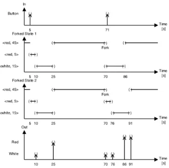
In Figure 2, we show the trajectories of a traffic light with pedestrians pushing the button at 5 and 71 seconds from the start of the simulation with no uncertainty intervals. Therefore, we know that at 71 seconds the traffic light will be on red and wait 45 seconds before turning back to white. In Figure 3, we repeated the previous simulation but this time using intervals of one second length for the input. Here, most of the time we are certain about the traffic light color, but for some moments we are in an uncertain color. For instance we cannot assert the light will be red at 71.5 seconds based in the collected data.
Figure 1: Trajectories of traffic light with no input
Figure 2: Trajectories of traffic light with input without uncertainty intervals
Figure 3: Trajectories of traffic light with input of 1 second accuracy
Something we would like to have in the future is a
mech-anism to trace each conflict back to their originating mea-surement, and be able to state what accuracy is needed to remove the ambiguity from the results to a level acceptable for the decision-making process. Having this kind of infor-mation can be used to replace instruments used in repetitive processes, for example in quality control jobs.
7.
CONCLUSIONS
We described the algorithms to simulate a subclass of DEVS models accepting input values measured with quantified un-certainty. Our algorithms produce all possible state and output trajectories for each possible value on the uncertainty intervals being used as input; this production only requires the addition of a finite set of simulators at each simulation step when simulating FF-DEVS models.
We characterized the DEVS subclass of FF-DEVS models and showed examples of which models belong to this sub-class. We compared FF-DEVS subclass against other known DEVS subclasses. We provided a case study to show how to use and what to expect from the algorithms as output. In our future work, we plan to explore new ideas to cover a larger subclass of DEVS models. We also want to work on a modeling language to simulate the introduction of uncer-tainty, for instance to introduce sensor models in the simu-lation. We want to provide the mechanisms for tracing back original measured input that resulted in a simulation branch. We want to explore optimization ideas to reduce the quan-tity of forks needed to simulate an FF-DEVS model using the proposed algorithms. Finally, we set our future goal to introduce uncertainty descriptions to the model. This ad-dition will allow exploiting the algorithms in new contexts were uncertainty is a characteristic of the system and not just an input.
8.
REFERENCES
[1] O. Aberth. Computable Calculus. Academic Press, 2001.
[2] R. Beraldi, L. Nigro, and A. Orlando. Temporal uncertainty time warp: an implementation based on java and actorfoundry. Simulation, 79(10):581–597, 2003.
[3] BIPM. Guide to the expression of uncertainty in measurement, (1995), with supplement 1, evaluation of measurement data, jcgm 101: 2008. Organization for Standardization, Geneva, Switzerland, 2008. [4] I. BIPM, I. IFCC, I. IUPAC, and O. ISO. The
international vocabulary of metrology—basic and general concepts and associated terms (vim), 3rd edn. jcgm 200: 2012. JCGM (Joint Committee for Guides in Metrology), 2008.
[5] A. Chow, B. P. Zeigler, and D. H. Kim. Abstract simulator for the parallel devs formalism. In AI, Simulation, and Planning in High Autonomy Systems, 1994. Distributed Interactive Simulation
Environments., Proceedings of the Fifth Annual Conference on, pages 157–163. IEEE, 1994.
[6] R. M. Fujimoto. Exploiting temporal uncertainty in parallel and distributed simulations. In Proceedings of the thirteenth workshop on Parallel and distributed simulation, pages 46–53. IEEE Computer Society,
1999.
[7] R. M. Fujimoto. Parallel simulation: parallel and distributed simulation systems. In Proceedings of the 33nd conference on Winter simulation, pages 147–157. IEEE Computer Society, 2001.
[8] A. Hernandez and N. Giambiasi. State reachability for devs models. In Proc. of Argentine Symposium on Software Engineering, 2005.
[9] M. H. Hwang and S. K. Cho. Timed behavior analysis of schedule preserved devs. In Proceedings of 2004 Summer Computer Simulation Conference, pages 26–29, 2004.
[10] M. H. Hwang and B. P. Zeigler. A modular
verification framework based on finite & deterministic devs. SIMULATION SERIES, 38(1):57, 2006. [11] M. Hybinette and R. Fujimoto. Cloning: a novel
method for interactive parallel simulation. In Proceedings of the 29th conference on Winter simulation, pages 444–451. IEEE Computer Society, 1997.
[12] M. Hybinette and R. M. Fujimoto. Cloning parallel simulations. ACM Transactions on Modeling and Computer Simulation (TOMACS), 11(4):378–407, 2001.
[13] M. Hybinette and R. M. Fujimoto. Scalability of parallel simulation cloning. In Simulation Symposium, 2002. Proceedings. 35th Annual, pages 275–282. IEEE,
2002.
[14] M. L. Loper and R. M. Fujimoto. Pre-sampling as an approach for exploiting temporal uncertainty. In Proceedings of the fourteenth workshop on Parallel and distributed simulation, pages 157–164. IEEE Computer Society, 2000.
[15] M. L. Loper and R. M. Fujimoto. A case study in exploiting temporal uncertainty in parallel
simulations. In Parallel Processing, 2004. ICPP 2004. International Conference on, pages 161–168. IEEE, 2004.
[16] R. E. Moore. Interval analysis, volume 4. Prentice-Hall Englewood Cliffs, 1966. [17] P. Peschlow and P. Martini. A discrete-event
simulation tool for the analysis of simultaneous events. In Proceedings of the 2nd international conference on Performance evaluation methodologies and tools, page 14. ICST (Institute for Computer Sciences, Social-Informatics and Telecommunications Engineering), 2007.
[18] B. P. Zeigler, H. Praehofer, and T. G. Kim. Theory of modeling and simulation: integrating discrete event and continuous complex dynamic systems. Academic press, 2000.
[19] B. P. Zeigler, H. Praehofer, T. G. Kim, et al. Theory of modeling and simulation, volume 19. John Wiley New York, 1976.