Cross-classification clustering : multi-object tracking technique for 3-D instance segmentation in connectomics

Cross-Classification Clustering:

Multi-Object Tracking Technique for 3-D Instance

Segmentation in Connectomics

by

Lu Mi

Submitted to the Department of Electrical Engineering and Computer Science

in partial fulfillment of the requirements for the degree of

Master of Science in Computer Science and Engineering at the

MASSACHUSETTS INSTITUTE OF TECHNOLOGY June 2019

0

Massachusetts Institute of Technology 2019. All rights reserved.

Signature redacted

A u th or ...

Department of Electrical Engineering and Computer Science May 20, 2019

Certified by...

Signature redacted

Nir Shavit Professor of Electrical E 7 eering and Computer Science Thesis Supervisor

Accepted by

...

Signature redacted....

' Lesdie

AVKolodziejski

Professor of Electrical Engineering and Computer Science Chair, Department Committee on Graduate Students

ARCHIVES OF TECHNOLOGY

JUN 13 2019

LIBRARIES

Cross- Classification Clustering: An Efficient Multi-Object Tracking Technique for 3-D Instance Segmentation in

Connectomics by

Lu Mi

Submitted to the Department of Electrical Engineering and Computer Science on May 20, 2019, in partial fulfillment of the

requirements for the degree of

Master of Science in Computer Science and Engineering

Abstract

In this thesis, cross- classification clustering (3C) is designed and implemented, it is a technique that simultaneously tracks complex, interrelated objects in an image stack. The key idea in cross-classification is to efficiently turn a clustering problem into a classification problem by running a logarithmic number of independent classi-fications per image, letting the cross-labeling of these classiclassi-fications uniquely classify each pixel to the object labels. The 3C mechanism was applied to achieve state-of-the-art accuracy in connectomics - the nanoscale mapping of neural tissue from electron microscopy volumes. This reconstruction system increases scalability by an order of magnitude over existing single-object tracking methods (such as flood-filling networks). This scalability is important for the deployment of connectomics pipelines, since currently the best performing techniques require computing infrastructures that are beyond the reach of most laboratories. This algorithm may offer benefits in other domains that require pixel-accurate tracking of multiple objects, such as segmentation of videos and medical imagery.

Thesis Supervisor: Nir Shavit

Title: Professor of Electrical Engineering and Computer Science

Acknowledgments

I would sincerely thank my advisor Prof. Nir Shavit, who decided to take me as his

student two years ago, then I would have chance to start my exciting journey into the area of Connectomics with his considerate support and thoughtful advise.

I would deeply thank my colleague Yaron Meirovitch who offers me great help and patient guidance when I was new to the area, and we had a wonderful collaboration on this segmentation project, and also I would also thank the help from my colleagues Hayk Saribekyan, Alexander Matveev, Shibani Santurkar, Jonanthan Rosenfeld.

I would like to thank my co-advisor Prof. Jeff Lichtman and Prof. Aravinthan Samuel from Harvard University to allow us to access the dataset of Connectomics, and they also offer a lot of support and guidance to my future graduate study.

I would gratefully thank Tianxing He and my dog Minnie, who are always great companion of the journey with me, and we share the happiness and overcome troubles together throughout the graduate life, which becomes much more fantastic than my expectation because of their attendance.

And finally, my ultimate gratitude goes to my parents and aunt who raise me selflessly, and educated me to become a happy and smart person, all of these would be not possible without their endless love.

Contents

1 Introduction 13 1.1 Related Work . . . . 16 1.2 C ontribution . . . . 18 1.3 Methodology . . . . 19 2 Experiments 25 2.1 SNEMI3D Dataset . . . . 25

2.2 Neural Network Details . . . . 27

2.3 Agglomeration. . . . . 28

2.4 Comparison with Baselines . . . . 31

3 Scalability Comparisons 33

List of Figures

1-1 (a) Single-object tracking using flood-filling networks [21], (b)

Multiple-object tracking using this cross-classification clustering (3C) algorithm, (c) The combinatorial encoding of an instance segmentation by 3C. One segmented image with 10 objects is encoded using three images, each w ith 4 object classes. . . . . 14 1-2 The raw input electron microscopy (EM) full image stack and the

3C-LSTM-UNET results in the SNEMI3D benchmark. . . . . 15

1-3 A high level view of the 3-D instance segmentation pipeline. . . . . . 19 1-4 The instance segmentation transfer mechanism of 3C: Encoding the

seeded image as k i-color images using the encoding rule x (k= log(N); here k=5 and 1=4). Applying a fully convolutional network k times to transfer each of the seed images to a respective target. Decoding the set of k predicted seed images using the decoding rule x -1. . . . 22 1-5 A schematic view of a global merge decision. The edge weight between

seed i and seed

j

at sections Z and Z+W, respectively. e is calculated by the ratio of the overlapping areas of seed j and the 3C prediction of seed i from images Z to Z+W. Seeds that over-segment a common object tend to get merged due to a path of strong edges. . 23

2-1 SNEMI3D: The 3C-LSTM-UNET architecture: Results compared with baseline techniques: Watershed, Neuroproof, and ground truth. . . . 26

2-2 A schematic view of the 3C networks. The input layers have 3 channels of the raw image, seed mask and border probability, for 2W+1 consecu-tive sections (images). The output is a feature map of seed predictions in section Z W (binary or labeled). Top: 3C-LSTM-UNET. Network architecture was implemented for the SNEMI3D dataset to optimize for accuracy. The inputs are processed with three consecutive Conv-LSTM modules, followed by a symmetric Residual U-Net structure. Bottom: 3C-Maxout. Network architecture was implemented for the

Harvard Rodent Cortex and PNS datasets to optimize for speed. . . . 27

2-3 SNEMI3D: The 3C-LSTM-UNET Results compared with baseline

tech-niques: Watershed, Neuroproof, and ground truth for sections Z=5, 25, 45, 65, 85. 32

3-1 Compute cost per pixel using FFN-Style segmentation. We computed the number of times a pixel is participating in object detection (red) for two public datasets (SNEMI3D, FlyEM), and compared to the number of classification calls in 3C. . . . . 34

List of Tables

2.1 Comparison of Watershed, Neuroproof

[41],

Multicut

[6],

human values,

3C and FFN [211 on the SNEMI3D dataset for Rand-Error, Variation of

Information VI, VI split, VI merge. Time Complexity: N is the number of objects and V is number of pixels. For empirical comparison see the performance section. I do not have access to the FFN and human outputs and hence their VI metric is missing . . . . 28

2.2 Different types of layers with its corresponding parameters, number of kernels, and kernel size for the 3C-MaxOut architecture used for the

S 1 dataset.. . . . . 29 2.3 Different types of layers with its corresponding parameters, number of

kernels, and kernel size for the 3C-MaxOut architecture used for the

P N S dataset. . . . . 29

2.4 Comparison of 3C-LSTM-UNET, 3C-UNET-LSTM,3C-UNET, 3C-Residual

UNET on SNEMI3D data for number of parameters, training accuracy

and validation accuracy. . . . . 30 2.5 Different types of layers with its corresponding parameters, number

of kernels and kernel size occur in module ConvLSTM and UNET for

Chapter 1

Introduction

Object tracking is an important and extensively studied component in many computer vision applications [1, 13,14, 16, 23, 53, 56, 58]. It occurs both in video segmentation and in 3-D object reconstruction based on 2-D images. Less attention has been given to efficient algorithms performing simultaneous tracking of multiple interrelated objects

[14]

in order to eliminate the redundancies of tracking multiple objects via repeated use of single-object tracking. This problem is relevant to applications in medical imaging [10, 11, 22,29,30, 38] as well as videos [12,43,54,57].

The field of connectomics, the mapping of neural tissue at the level of individual neurons and the synapses between them, offers one of the most challenging settings for testing algorithms to track multiple complex objects. Such synaptic level maps can be made only from high-resolution images taken by electron microscopes, where the sheer volume of data that needs to be processed (petabyte-size image stacks), the desired accuracy and speed (terabytes per hour

[331),

and the complexity of the neurons' morphology, present a daunting computational task. By analogy to traditional object tracking, imagine that instead of tracking a single sheep through multiple video frames, one must track an entire flock of sheep that intermingle as they move, change shape, disappear and reappear, and obscure each other

[321.

As a consequence of this complexity, several highly successful tracking approaches from other domains, such as the "detect and track" approach [14], are less immediately applicable to connectomics.

(a)

Proposal

(b)

Source Single Object Mask

Proposal

Source Multi-Objects Mask

Evidence

Source Images Borders

Evidence

Source Images Borders

(c) Encoding of Instance Segmentation by 3C

Instance Segmentation

6

Prediction

FCN Single-Mask Prediction on Target Images

Prediction

3C

Multi-Mask Prediction on Target Images En oednt stance Segmentation x

Figure 1-1: (a) Single-object tracking using flood-filling networks [21], (b) Multiple-object tracking using this cross-classification clustering (3C) algorithm, (c) The com-binatorial encoding of an instance segmentation by 3C. One segmented image with

SNEMI3D benchmark test dataset

Raw input

Full Stack of Electron Microscopy(EM) images (100 slices)

3C-LSTM-UNET result

Figure 1-2: The raw input electron microscopy (EM) full image stack and the

3C-LSTM-UNET results in the SNEMI3D benchmark.

Certain salient aspects are unique to the connectomics domain: a) All objects are of the same type (biological cells); sub-categorizing them is difficult and has little relevance to the segmentation problem.

b) Most of the image is foreground, with tens to hundreds of objects in a single

megapixel image. c) Objects have intricate, finely branched shapes and no two are the same. d) Stitching and alignment of images can be imperfect, and the distance between images (z-resolution) is often greater than between pixels of the same image (xy-resolution), sometimes breaking the objects' continuity. e) Some 3-D objects are laid out parallel to the image stack, spanning few images in the z direction and going back and forth in that limited space with extremely large extensions in some image planes.

In this work, a 3C technique is introduced, that achieves volumetric instance segmentation by transferring segmentation knowledge from one image to another, simultaneously classifying the pixels of the target image(s) with the labels of the

matching objects from the source image(s).

This algorithm is optimized for the setting of connectomics, in which objects frequently branch and come together, but is suitable for a wide range of video-segmentation and medical imaging applications.

The main advantage of the solution is its ability, unlike prior single-object tracking methods for connectomics [21,37], to simultaneously and jointly segment neighboring, intermingled objects, thereby avoiding redundant computation. In addition, instead of extending single masks, the detectors perform clustering by taking into account information on all visible objects.

The efficiency and accuracy of 3C are demonstrated on four connectomics datasets: the public SNEMI3D benchmark dataset, shown in Figure 1-2, the widely studied mouse somatosensory cortex dataset

[24]

(Si), a Lichtman Lab dataset of the V1

region of the rat brain (ECS), and a newly aligned mouse peripheral nervous system dataset (PNS), where possible, comparing to other competitive results in the field of connectomics.

1.1

Related Work

A variety of techniques from the past decade have addressed the task of neuron

seg-mentation from electron microscopy volumes. An increasing effort has been dedicated to the problem of densely segmenting all pixels of a volume according to foreground object instances (nerve and support cells), known as saturated reconstruction. Note that unlike everyday images, a typical megapixel electron microscopy image may con-tain hundreds of object instances, with very little background (<10%). Below, the saturated reconstruction pipelines are briefly surveyed that seem to us most influential and related to the approach undertaken here.

Algorithms for saturated reconstruction of connectomics data have proved most accurate when they combine many different machine learning techniques

[6,31].

Many of these techniques use the hierarchical approach of Andres et al.

[2]

that employs the well-known hierarchical image segmentation framework

[3,15,

39,46].

This is still the most common approach in connectomics segmentation pipelines: first detecting object borders in 2-D/3-D and then gradually agglomerating informa-tion to form the final objects [6,9,20,27,31,34,35,51]. The elevainforma-tion maps obtained from the border detectors are treated as estimators of the true border probabilities

_[91,

which are used to define an over-segmentation of the image, foreground conrected components on top of a background canvas. The assumption is that each of the con-nected components straddles at most a single true object. Therefore it may need to be agglomerated with other connected components (heuristically

[17,18,261

or based on learned weights of hand-crafted features

[2,

27,40, 41]), but it should not be

bro-ken down into smaller segments. Numerous 3-D reconstruction systems follow this bottom-up design [6, 7,27,31,35,40,41, 44].

A heavily engineered implementation of hierarchical segmentation [31] still

occu-pies the leading entry in the (still active) classical SNEMI3D connectomics contest of

2013 [5], evaluated in terms of the uniform instance segmentation correctness metrics

(normalized Rand-Error [52] and Variation of Information [36]).

A promising new approach was recently taken with the introduction of flood-filling

networks (FFN; [21]) by Januszewski et al. and concurrently and independently of MaskExtend [37] by Meirovitch et al. As seen in Figure 1-1(a), these algorithms take a mask defining the object prediction on a source image(s), and then use a fully con-volutional network (FCN) to classify which pixels in the target image(s) belong to the singly masked object of the source image(s). This process is repeated throughout the image stack in different directions, segmenting and tracking a single object each time, while gradually filling the 3-D shape of complex objects. This provides accu-racy improvements on several benchmarks and potentially tracks objects for longer distances [21] compared to previous hierarchical segmentation algorithms (e.g., [6]).

However, these single-object trackers are not readily deployable for large-scale appli-cations, especially when objects are tightly packed and intermingled with each other, because then individual tracking becomes highly redundant, forcing the algorithm to revisit pixels of related image contexts many times1. Furthermore, the

ing single-object detectors in connectomics 121,37] and in other biomedical domains (e.g. [4, 8, 19, 47]) do not take advantage of the multi-object scene to better under-stand the spatial correlation between different 3-D objects. The approach taken here generalizes the single-object approach in connectomics to achieve simpler and more effective instance segmentation of the entire volume.

1.2

Contribution

This work provides a scalable framework for 3-D instance segmentation and multi-object tracking applications, with the following contributions:

" It proposes a simple FCN approach, tackling the less studied problem of

map-ping an instance segmentation between two related images. The algorithm jointly predicts the shapes of several objects partially observed in the input. " It proposes a novel technique that turns a clustering problem into a classification

problem by running a logarithmic number of independent classifications on the pixels of an image with N objects (for possibly large N, bounded only by the number of pixels).

* It shows empirically that the simultaneous tracking ability of this algorithm is more efficient than independently tracking all objects.

* It conducts extensive experimentation on public benchmark connectomics dataset

SNEMI3D, under different evaluation criteria and a performance analysis, to

show the efficacy and efficiency of the technique on the problem of neuronal reconstruction.

Data Space Step 1

Seeder

FCN Step

Me

gmOp-Segmented Space

Seeded Space (integers)

k -color Seeded Space

Step 2 1 k

Encoder

...

x:

randomized

N seeds k= log(N) (Over-segmentation) Label _SCN ste A

Transfer

I

rger Transferred seeds

Decoder

x-

1 1 k

k i-color Seeded Spaces

Figure 1-3: A high level view of the 3-D instance segmentation pipeline.

1.3

Methodology

This work presents cross-classification clustering (henceforth 3C), a technique that extends single object classification approaches, simultaneously and efficiently classi-fying all objects in a given image based on a proposed instance segmentation of a context-related image. One can think of the context-related image and its segmenta-tion as a collecsegmenta-tion of labeled masks to be simultaneously remapped together to the new target image, as in Figure 1-1(b). The immediate difficulty of such simultaneous settings is that this generalization is a clustering problem: unlike FFNs and MaskEx-tend (shown in Figure 1-1(a)), that produce a binary output ("YES" for exMaskEx-tending the object and otherwise "NO"), in any volume, we really do not know how many classification labels we might need to capture all the objects, or more importantly how to represent those instances in ways usable for supervised learning. Overcoming this difficulty is a key contribution of 3C.

Cross-Classification Clustering: To begin with, the main idea is described behind 3C and differentiating it from single-object methods such a FFNs. Then a

top-down sketch of the pipeline is provided and described about how it can be adapted to other domains.

s

The goal is to extend a single-object classification from one image to the next so as to simultaneously classify pixels for an a priori unknown set of object labels.

More formally, suppose that we have images Xprev and Xext, where Xprev has been

segmented and Xnext must be segmented consistent with Xprev. Given two such

images, we seek a classification function f that takes as input a voxel v of Xext and a segmentation s of Xprev (an integer matrix representing object labels) and outputs a decision label. The function

f

outputs a label if and only if v belongs to the object with that label in s. If s is allowed to be an over-segmentation (i.e., several labels representing the same object) then the output of

f

should be one of the compatible labels.

For simplicity, let us assume that the input segmentation s has entries from the

label set

{1,

... , _{N}. We define a new space of labels, the length-k strings over a}

predetermined alphabet A (here represented by colors), where JAI = 1 and n-Alk k

N is an upper bound on the number of objects we expect in a classification. We use

an arbitrary encoding function, x, that maps labels in

{

1, --- , N} to distinct random

strings over A of length k. In the example in Figure 1-1(c), A is represented by 1=4

colors, and k=3, so we have a total of 43=64 possible strings of length 3 to which the

N=10 objects can be mapped. Thus, for example, object 5 is mapped to the string

(Green, Purple, Orange) and object 1 is (Green, Green, Purple). We can define the classification function

f

on string labels as the product of k traditional classifications, each with an input segmentation of labels in A, and an output of labels in A. Slightly

abusing notation, let the direct product of images x(s) = X1(s) x ... x Xk(s) be the

relabeling of the segmentation s where each image (or tensor) Xi(s) is the projection of x(s) in the i-th location (a single coloring of the segmentation) and x is the concatenation operation on labels in A. Then we can re-define

f

on x(s) as

f (v, x(s)) = f'(v, Xi(s)) x - x f'(v,Xk(s)), (1.1)

where each f'(Xk(s)) is a traditional classification function. The key idea is that

labels. In the example in Figure 1-1(c), even though in the map representing the most significant digit of the original objects 5 and 1, they are both Green, when we perform the classification and take the cross labeling of all three maps, the two objects are classified into distinct labels.

3-D reconstruction system: The 3-D reconstruction system consists of the

following steps (shown in Figure 1-3):

1) Seeding and labeling the volume with an initial imperfect 2-D/3-D instance

seg-mentation that overlaps all objects except for their boundaries (over-segseg-mentation). 2) Encoding the labeled seeds into a new space using the 3C rule

x.

3) Applying a fully convolutional network log(N) times to transfer the projected

labeled seeds from the source image to the target images, and then take their cross labeling.

4) Decoding the set of network outputs to the original label space using the inverse

3C rule

x

1 .

5) Agglomerating the labels into 3-D consistent objects based on the overlap of

the original seeding and the segments predicted from other sections.

To initially seed and label the volume (Step 1), the 2-D masks are computed and labeled that over-segment all objects. For this, it follows common practice in connectomics, computing object borders with FCNs and searching for local minima in 2-D on the border elevation maps. Subsequently (Step 2), x is used to encode the seeds of each section, resulting in a k-tuple over the i-color alphabet for each seed

(k=5 and 1=4 in Figure 1-4).

A fully convolutional neural network then predicts the correct label mapping

be-tween interrelated images of sections Z and Z W, which determines which pixels in target image Z W belong to which seeds in source image Z (step 3). All seeds here are represented by a fixed number I of colors, and prediction is done log(N) times based on Equation 1.1. For decoding, all log(N) predictions are aggregated for each pixel to determine the original label of the seed using

x

1 _{(Step 4). For training, I}

use saturated ground truth of the 3-D consistent objects. This approach allows us to formalize the reconstruction problem as a tracking problem between independent

3C Input

Section Z Section Z Section Z+ W

!

Prior Segmentation Prior EM Current EM (multi color) Source image Target image Encoding

3C Output

Section Z W Segmentation (muti color) Decoding/ FCN argmax Call 2 FCN -argmax 01 FCN argmax FCN argmax Call 5 FCN argmax

class 1 class 2 class 3 class 4

Figure 1-4: The instance segmentation transfer mechanism of 3C: Encoding the seeded image as k i-color images using the encoding rule x (k= log(N); here k=5 and 1=4). Applying a fully convolutional network k times to transfer each of the seed images to a respective target. Decoding the set of k predicted seed images using the decoding rule

X-Global decision of merge according to strong edges

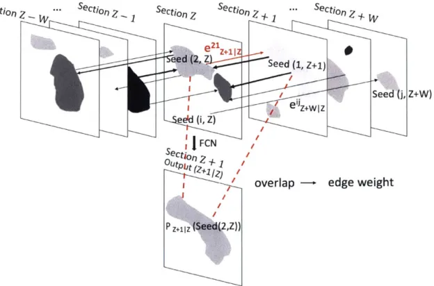
Sectio Seed (2, Z ee'd (i, Z) FCN Section _Z Outpt (Z+L +z /Z) P z+ (Seed (2,Z)) I . Section _{Z + W} V Seed (1, z+1) overlap I W I Seed edge weight

Figure 1-5: A schematic view of a global merge decision. The edge weight between seed i and seed

j

at sections Z and Z+W, respectively. e" z is calculated by the

ratio of the overlapping areas of seed

j

and the 3C prediction of seed i from images

Z to Z+W. Seeds that over-segment a common object tend to get merged due to a

path of strong edges.

Section _z - _... Section

Z

(j,lZ+W)

images, and to deal with the tendency of objects to disappear/appear in different portions of an enormous 3-D dataset.

Now how the 3C seed transfers are utilized to agglomerate the 2-D masks (as shown in Figure 1-5) is described. For agglomeration (Step 5), the FCN for 3C is applied from all source images to their target images, which are at most W image sections apart from each other across the image stack (along the z dimension). I then collect overlaps between all co-occurring segments, namely, those occurring by the original 2-D seeding, and those by the 3C seed transfer from source to target images. This leaves 2W+1 instance segmentation cases for each image (including the initial seeding), which directly link seeds of different sections. Formally, the overlaps of different labels define a graph whose nodes are the 2-D seed mask labels and the directed weighted edges are their overlap ratio from the source to the target. Instead of optimizing this structure (as in the Fusion approach of

[25]),

I found that agglomerating all masks of sufficient overlap delivers adequate accuracy even for a small W. We do however make forced linking on lower probability edges to avoid "orphan" objects that are too small, which is biologically implausible.

To note that 3C does not attempt to correct potential merge errors in the initial seeding, these can be addressed post-hoc by learning morphological features [48, 59]

or global constraints [34].

Adaptation to other domains: To leverage 3C for multi-object tracking in

videos, a domain-specific seeder should precede cross classification (e.g. with deep coloring [28]). Natural images are likely to introduce spatially consistent object splits across frames and hence a dedicated agglomerating procedure should follow. The 3C technique can be readily applied to other medical imaging tasks, with seed transfers across different axes for isotropic settings.

Chapter 2

Experiments

The SNEMI3D challenge is a widely used benchmark for connectomic segmentation algorithms dealing with anisotropic EM image stacks [5]. Although the competition ended in 2014, several leading labs recently submitted new results on this dataset, improving the state-of-the-art. Recently Plaza et al. suggested that benchmarking connectomics accuracy on small datasets as SNEMJ3D is misleading as large-scale "catastrophic errors" are hard to assess [44, 45]. Moreover, the clustering metrics such as Variation of Information

[36]

and Rand Error [52] are inappropriate since they are not centered around the connectomics goal of unraveling neuron shape and inter-neuron connectivity. Therefore experiments are conducted on three additional datasets and show the Rand-Error results only on the canonical SNEMI3D dataset, which has the corresponding Ground Truth labels.

2.1

SNEMI3D Dataset

In order to implement 3C on the SNEMI3D dataset, I firstly created an initial set of

2-D labeled seeds over the entire volume. These were generated based on the regional 2-D minima of the border probability map. This map was generated by a Residual

U-Net, which is known for its excellent average pixel accuracy in border detection [31,49]. Next, the 3C algorithm was used to transfer 2-D labeled seeds through the volume, as shown in Figure 1-4. Finally, the original 2-D labeled seeds and transferred labeled

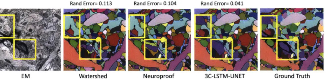
Rand Error= 0.113 Rand Error= 0.104 Rand Error= 0.041

EM Watershed Neuroproof 3C-LSTM-UNET Ground Truth

Figure 2-1: SNEMI3D: The 3C-LSTM-UNET architecture: Results compared with baseline techniques: Watershed, Neuroproof, and ground truth.

seeds were agglomerated if their overlap ratio exceeded 0.1. I found that W=2 delivers adequate accuracy. All orphans were greedily agglomerated to their best match. In order to achieve better accuracy, I tested 3C with various network architectures, and evaluated their accuracy. To date, convolutional LSTMs (ConvLSTM) have shown good performance for sequential image data

[55].

In order to adapt these methods to the high pixel-accuracy required for connectomics, I combined both ConvLSTM and U-Net. The network is trained to learn an instance segmentation of one image based on the proposed instance segmentation of a nearby image with similar context.

I found that the LSTM-UNET architecture has validation accuracy of 0.961, which

outperforms other commonly used architectures. A schematic view of the architecture is given in Figure 2-2.

In order to illustrate the accuracy of 3C, I submitted the result to the public SNEMI3D challenge website alongside two common baseline models, the 3-D water-shed transform (a region-growing technique) and Neuroproof agglomeration

[41].

The watershed code was adopted from

[35].

Similar to other traditional agglomerating-techniques, Neuroproof trains a random forest on merge decisions of neighboring objects 140-42]. These baseline methods were fed with the same high-quality border maps used in the 3C reconstruction system. The comparisons of 2-D results with ground truth (section Z=30) are shown in Figure 2-1. The result has fewer merge-and split-errors, merge-and outperforms the two baselines by a large margin. Furthermore,

3C compares favorably to other state of art works recently published in Nature

3C-LSTM-UNET

Section Z Section Z - W Section Z W

Section Z - 1 Class 1

Class 1 seed map _{ss sed apSection Z} Sectio ~ . C oRes Prediction

-- v-Conv -ResidualP dbb Mp

Border Section Z + 1 2D 2D 20a

EM ImeSection Z + W S12x512x1

(2W + 1)x512x512x3

3C-Maxout Section z 4 matrices 16 matrices 64 matrices 128 matrices _{Section Z W}

-.. .5 Classes

Class [0, 41 label Conv Conv No Object

map : Max . x Max Object Colored 1

EM Image N Object Colored 2

Border

-* -* -Object Colored 3

1027x1027x1 Object Colored 4

1069x1069x(2W + 1)x3 533x533 265x265 131x131 64x64

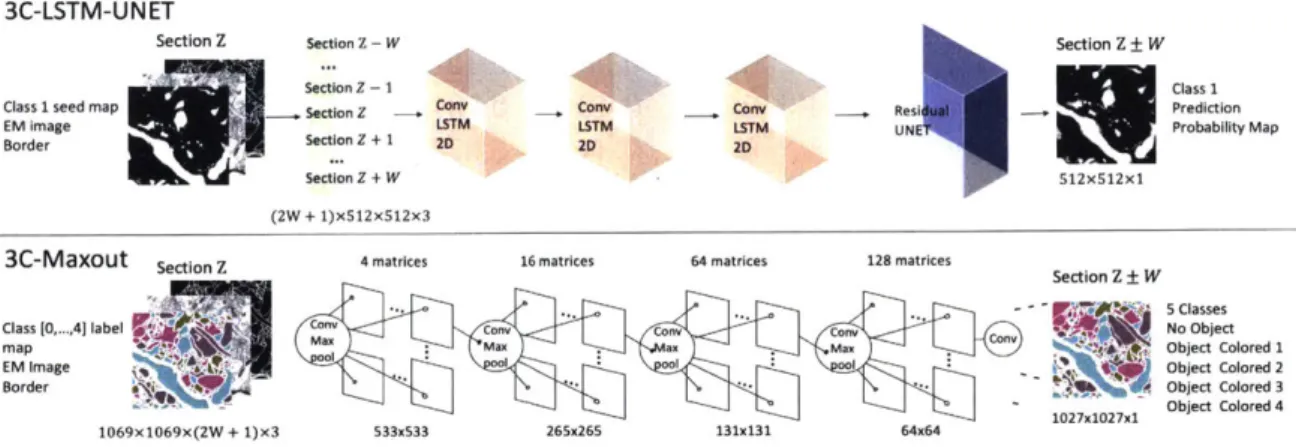
Figure 2-2: A schematic view of the 3C networks. The input layers have 3 channels of the raw image, seed mask and border probability, for 2W+1 consecutive sections (images). The output is a feature map of seed predictions in section Z W (binary

or labeled). Top: 3C-LSTM-UNET. Network architecture was implemented for the

SNEMI3D dataset to optimize for accuracy. The inputs are processed with three

consecutive Conv-LSTM modules, followed by a symmetric Residual U-Net structure.

Bottom: 3C-Maxout. Network architecture was implemented for the Harvard Rodent Cortex and PNS datasets to optimize for speed.

compared with the 0.06 achieved by a human annotator. The accuracy (ranked 3rd) outperforms most of the traditional pipelines many by a large margin, and is slightly behind the slower neuron-by-neuron FFN segmentation for this volume. The leading entry is a UNET-based model learning short and long range affinities [31]. The results are summarized in Table 2.1.

2.2

Neural Network Details

Three types of network architecture were studied: 1) 3C-Maxout, a light Maxout network [351 used for the large-scale experiment with the S1 dataset [24]. It has 6 output classes (1-4 3C colors, border prediction, new-object-prediction), and a

FoV=109x109. The input has 16 feature maps, encoding the 1 colors as equilaly

space fractions between 0 and 1. I used 1 = 4. Each module includes a cascade of 64 4x4 convolutions, 2x2 maxpool and a maxout, as shown in Table 2.2. 2) An even lighter 3C-Maxout network was used for the PNS dataset. It has 5 outpus classes (1-4 colors, not-axon), and FoV=53x53, the input has 16 feature maps. The same

Table 2.1: Comparison of Watershed, Neuroproof

[41],

Multicut

[61,

human values, 3C and FFN [21] on the SNEMI3D dataset for Rand-Error, Variation of Information VI, VI split, VI merge. Time Complexity: N is the number of objects and V is number of pixels. For empirical comparison see the performance section. I do not have access to the FFN and human outputs and hence their VI metric is missing.

structure is used as in 1), with half the features and a shallower network, as shown in Table 2.3. 3) A module combination of convLSTM and UNET which ix called 3C-LSTM-UNET. It has 4 classes (1-4 colors), and FoV=512x512. Here I only report

on the different types of layers included in this architecture, as shown in Table 2.5.

My implementation of 3C-LSTM-UNET for the SNEMI3D dataset used Keras

with Tensorflow backend. All experiments are run on a server with a single Tesla

V100-PCIE GPU. I trained the model by minimizing binary-entropy through

back-propagation, using Adam with a learning rate of 10-4. The implementation of 3C-Maxout for the PNS and S1 experiment used SGD solver in Caffe with a learning

rate of 7 -10-3.

I further compared the accuracy and number of parameters of 3C-LSTM-UNET with other commonly used network structures, such as UNET and Residual UNET, results are shown in Table 2.4.

2.3

Agglomeration

The agglomeration step merges a 2-D seed with a seed propagated by the 3C al-gorithm, if the two segments overlap for at least 1/10 of the area of the originally placed seed. After the agglomeration step is terminated, some objects with biolog-ically implausible properties, such as a small volume, improbable object flatness or

Model

[

Rand VI Vlspiit

[

VImerge I Complexity

Watershed 0.113 0.67 0.55 0.12 Neuroproof 0.104 0.55 0.42 0.13 Multicuts 0.068 0.41 0.34 0.07 3C 0.041 0.31 0.19 0.12 O(V log N) FFN 0.029 - - - O(VN) Human val. 0.060 - -

-Type Number Kernel

/layers

of kernels size/Stride

convI 128 4x4/1 maxpool - 2x2/2 maxout 2:1 -conv2 128 4x4/1 maxpool - 2x2/2 maxout 2:1 -conv3 128 4x4/1 maxpoo - 2x2/2 maxout 2:1 -conv4 128 4x4/1 maxpool - 2x2/2 maxout 2:1 -conv5 6 4x4/1

Table 2.2: Different types of layers with its corresponding parameters, number of kernels, and kernel size for the 3C-MaxOut architecture used for the S1 dataset.

Type Number Kernel

/layers

of kernels size/Stride

convI 64 4x4/1 maxpool - 2x2/2 maxout 2:1 -conv2 64 4x4/1 maxpool - 2x2/2 maxout 2:1 -conv3 64 4x4/1 maxpool - 2x2/2 maxout 2:1 -conv4 5 4x4/1

Table 2.3: Different types of layers with its corresponding parameters, number of kernels, and kernel size for the 3C-MaxOut architecture used for the PNS dataset.

Table 2.4: Comparison of Residual UNET on SNEMI3D validation accuracy.

3C-LSTM-UNET,

data for number of

3C-UNET-LSTM,3C-UNET,

3C-parameters, training accuracy and

Table 2.5: Different types of layers with its corresponding parameters, number of kernels and kernel size occur in module ConvLSTM and UNET for construction of

3C-LSTM-UNET architecture.

Network Structure Number of Training/Validation

Parameters Accuracy

3C-LSTM-UNET 4M 0.963/0.961 3C-UNET-LSTM 4M 0.861/0.864

3C-UNET 31M 0.881/0.880

3C-Residual UNET 17M 0.915/0.863

Module Type Number Kernel

/Layer of kernels size/Stride

ConvLSTM convLSTM 20 3 x 3/1 BN - -conv1 32 3x3/1 conv2 64 3x3/1 conv3 128 3x3/1 conv4 256 3x3/1 UNET conv5 512 3x3/1 conv6 1 1xl/1 BN - -maxpool - 2x2/2 upsample - 2x2/1

impossible topology may occur. The problem of error detection in connectomics is not

widely studied and is poorly understood, although recently several works suggested data-driven approaches to the problem, for example learning and detecting the

mor-phology of implausible objects [48,59]. Others applied a model-based approach for

example for detecting biologically an implausible object topology of an X-junction [37] or by learning local and non-local biological constraints [34].

Orphans are objects that reside within the dataset but are either very small or

do not reach the boundaries of the volume. For teravoxel mammalian-cortex connec-tomics, all final objects (neuronal compartments) must be large enough to reach the boundary of dataset. Thus, all orphans are incorrect split objects which if possible needs to be merged to other split or orphan objects.

In this work a simple heuristic is used to avoid the existence of any orphan in the dataset. All orphans are marked and then iteratively merged the strongest edge between an orphan and a non-orphan object, where weighted edges are defined by the 3C algorithm. In the end, if the dataset still contained orphans, the closest pair of an orphan and a non-orphan objects is iteratively connected, by measuring distance

on the affinity graph with the weighted edges defined by the border probability map.

2.4

Comparison with Baselines

Here I supplement the comparison from the main text for the SNEMI3D experiment. I provide additional 2-D results for sections Z=5, 25, 45, 65, 85, generated from the 3C-LSTM-UNET network, with the same ground truth and the two baselines reported in the main text, Neuroproof [40-42] and Watershed

[35].

The results are shown in Figure 2-3. Each segmented image is provided with the corresponding value of Variation of Information (VI) [36].

EM image Watershed Neuroproof 3C-LSTM-UNET Ground Truth

Z=5VI = 0.318 VI=0.282 VI=0.065

Z=25 VI =0.304 VI =0.259 VI =0.154

Z=45 VI =0.423 VI =0.342 VI =0.244

Z=65 VI =0.424 VI =0.395 VI =0.187

Z=85 VI =0.204 VI =0.189 VI =0.080

Figure 2-3: SNEMI3D: The 3C-LSTM-UNET Results compared with baseline tech-niques: Watershed, Neuroproof, and ground truth for sections Z=5, 25, 45, 65, 85.

Chapter 3

Scalability Comparisons

In this section, the relative scalability of 3C to FFN and MaskExtend is compared, as far as possible without having access to the full FFN pipeline. 3C is a generalization of the FFN and MaskExtend techniques [21,37], which augment the (pixel) support set of each object, one at a time. The 3C technique simultaneously augments all the objects from its input image(s) after a logarithmic number of iterations (see Figure 1-4). This allows us directly to compare based on the number of iterations required, ignoring details of implementation.

FFN: The number of FCNs calls are compared in FFN and 3C assuming both

algorithms reconstruct all objects flawlessly. Both algorithms are assumed to use the same FCN model. Although 3C and FFN invoke FCNs a logarithmic versus a linear number of times, respectively, FFN runs on smaller inputs, centered around small regions of interest. At each iteration, FFN will output an entire 3-D mask of the object around the center pixel. A fraction of those pixels are assumed to require revisiting (zero for best-case scenario). Figure 3-1 depicts the number of FCN calls and their ratio for FlyEM [50] and SNEMI3D [5] for FFN and 3C. In 3C, each pixel participates in an FCN call a number of times logarithmic in the number of objects visible in the field of view (the FCN calls for FFN are color-coded red in the data cubes of Figure 3-1). The y-axis depicts the ratio between the FCN calls by 3C to that for FFN, for several ratios of object pixels found per FCN call. A zero ratio means that no pixels are found for the object in a single FCN call, whereas 1 means

Performance Analysis: FFN & 3C Comparison

Number of FCN calls in FFN 112 FCN calls 1 FCN call 19 FCN calls 1 F1 FCN call 199 FCN calls -FCN call 29 FCN calls FCN call SNEMI3D FlyEM ---U U-.-U U

z

0 0 z~ U LL '4-0 (-)

0

0.1

0.2

0.3

0.4

0.5

0.6

0.7

0.8

0.9

Average ratio of object pixels found per FCN call

Figure 3-1: Compute cost per pixel using FFN-Style segmentation. We computed the number of times a pixel is participating in object detection (red) for two public datasets (SNEMI3D, FlyEM), and compared to the number of classification calls in

3C. U U - I I __I 100

80

60

40

20

0

1

that all object pixels are found and require no further revisiting. It can see from the plot that, assuming error-free reconstruction, 3C is more efficient than FFN when there is a fraction of object pixels that require revisiting after a single call of the

FCN. The revisiting of some pixels is also reported by [211, as the 3-D output has

greater uncertainty far from the initial pixels. For a revisit ratio of 0.5, 3C is more than 10x faster than FFN on FlyEM.

Chapter 4

Conclusion

In this work, the cross-classification clustering (3C) is presented, it is an algorithm

that tracks multiple objects simultaneously, transferring a segmentation from one

image to the next by composing simpler segmentations. The power of 3C is demon-strated in the domain of connectomics, which presents an especially difficult task for

image segmentation.

Within the space of connectomics algorithms, 3C provides an end-to-end approach with fewer "moving parts", improving on the accuracy of many leading connectomics systems. The solution is computationally cheap, can be achieved with lightweight FCNs, and is at least an order of magnitude faster than its relative, flood-filling

net-works. Although the main theme of this work was tackling neuronal reconstruction, this approach also promises scalable, effective algorithms for broader applications in medical imaging and video tracking.

Bibliography

[1]

Amit Adam, Ehud Rivlin, and Ilan Shimshoni. Robust fragments-based tracking using the integral histogram. In Computer vision and pattern recognition, 2006

IEEE Computer Society Conference on, volume 1, pages 798-805. IEEE, 2006.

[2]

Bj6rn Andres, Ullrich K6the, Moritz Helmstaedter, Winfried Denk, and Fred A Hamprecht. Segmentation of SBFSEM volume data of neural tissue by hierar-chical classification. In Joint Pattern Recognition Symposium, pages 142-152. Springer, 2008.

[3]

Pablo Arbelaez, Michael Maire, Charless Fowlkes, and Jitendra Malik. Contour detection and hierarchical image segmentation. Pattern Analysis and Machine

Intelligence, IEEE Transactions on, 33(5):898-916, 2011.

[4] Assaf Arbelle, Jose Reyes, Jia-Yun Chen, Galit Lahav, and Tammy Riklin Ra-viv. A probabilistic approach to joint cell tracking and segmentation in high-throughput microscopy videos. Medical image analysis, 47:140-152, 2018.

[5]

Ignacio Arganda-Carreras, Srinivas C Turaga, Daniel R Berger, Dan Ciregan, Alessandro Giusti, Luca M Gambardella, Jilrgen Schmidhuber, Dmitry Laptev, Sarvesh Dwivedi, Joachim M Buhmann, et al. Crowdsourcing the creation of image segmentation algorithms for connectomics. Frontiers in neuroanatomy, 9:142, 2015.

[6]

Thorsten Beier, Constantin Pape, Nasim Rahaman, Timo Prange, Stuart Berg, Davi D Bock, Albert Cardona, Graham W Knott, Stephen M Plaza, Louis K Scheffer, et al. Multicut brings automated neurite segmentation closer to human performance. Nature Methods, 14(2):101-102, 2017.

[7]

Manuel Berning, Kevin M Boergens, and Moritz Helmstaedter. SegEM: efficient image analysis for high-resolution connectomics. Neuron, 87(6):1193-1206, 2015.

[8]

Ryoma Bise, Takeo Kanade, Zhaozheng Yin, and Seung-il Huh. Automatic cell tracking applied to analysis of cell migration in wound healing assay. In 2011

An-nual International Conference of the IEEE Engineering in Medicine and Biology Society, pages 6174-6179. IEEE, 2011.

[9]

Dan Ciresan, Alessandro Giusti, Luca M Gambardella, and Jiirgen Schmidhu-ber. Deep neural networks segment neuronal membranes in electron microscopy

images. In Advances in neural information processing systems, pages 2843-2851, 2012.

[10]

Qi

Dou, Lequan Yu, Hao Chen, Yueming Jin, Xin Yang, Jing Qin, and Pheng-Ann Heng. 3d deeply supervised network for automated segmentation of volu-metric medical images. Medical image analysis, 41:40-54, 2017.

111] Michal Drozdzal, Gabriel Chartrand, Eugene Vorontsov, Mahsa Shakeri, Lisa

Di Jorio, An Tang, Adriana Romero, Yoshua Bengio, Chris Pal, and Samuel Kadoury. Learning normalized inputs for iterative estimation in medical image segmentation. Medical image analysis, 44:1-13, 2018.

[121 Loic Fagot-Bouquet, Romaric Audigier, Yoann Dhome, and Fr6d6ric Lerasle. Improving multi-frame data association with sparse representations for robust near-online multi-object tracking. In European Conference on Computer Vision, pages 774-790. Springer, 2016.

[13]

Jialue Fan, Wei Xu, Ying Wu, and Yihong Gong. Human tracking using convo-lutional neural networks. IEEE Transactions on Neural Networks,

21(10):1610-1623, 2010.

[14]

Rohit Girdhar, Georgia Gkioxari, Lorenzo Torresani, Manohar Paluri, and Du Tran. Detect-and-track: Efficient pose estimation in videos. In Proceedings

of the IEEE Conference on Computer Vision and Pattern Recognition, pages

350-359, 2018.

[151

Kostas Haris, Serafim N Efstratiadis, Nikolaos Maglaveras, and Aggelos K Kat-saggelos. Hybrid image segmentation using watersheds and fast region merging.

IEEE Transactions on image processing, 7(12):1684-1699, 1998.

[16]

David Held, Sebastian Thrun, and Silvio Savarese. Learning to track at 100 fps with deep regression networks. In European Conference on Computer Vision, pages 749-765. Springer, 2016.

[17]

Moritz Helmstaedter. Cellular-resolution connectomics: challenges of dense neu-ral circuit reconstruction. Nature methods, 10(6):501-507, 2013.

[18] Moritz Helmstaedter, Kevin L Briggman, Srinivas C Turaga, Viren Jain, H

Se-bastian Seung, and Winfried Denk. Connectomic reconstruction of the inner plexiform layer in the mouse retina. Nature, 500(7461):168, 2013.

[19]

Nathaniel Huebsch, Peter Loskill, Mohammad A Mandegar, Natalie C Marks, Alice S Sheehan, Zhen Ma, Anurag Mathur, Trieu N Nguyen, Jennie C Yoo, Luke M Judge, et al. Automated video-based analysis of contractility and calcium flux in human-induced pluripotent stem cell-derived cardiomyocytes cultured over different spatial scales. Tissue Engineering Part C: Methods, 21(5):467-479, 2015.

[201

Viren Jain, Joseph F Murray, Fabian Roth, Srinivas Turaga, Valentin Zhigulin, Kevin L Briggman, Moritz N Helmstaedter, Winfried Denk, and H Sebastian Seung. Supervised learning of image restoration with convolutional networks. In

Computer Vision, 2007. ICCV 2007. IEEE 11th International Conference on,

pages 1-8. IEEE, 2007.

[21] Michal Januszewski, J6rgen Kornfeld, Peter H Li, Art Pope, Tim Blakely, Larry Lindsey, Jeremy Maitin-Shepard, Mike Tyka, Winfried Denk, and Viren Jain. High-precision automated reconstruction of neurons with flood-filling networks.

Nature methods, 15(8):605, 2018.

[22] Alexandr A Kalinin, Ari Allyn-Feuer, Alex Ade, Gordon-Victor Fon, Walter Meixner, David Dilworth, Jeffrey R De Wet, Gerald A Higgins, Gen Zheng, Amy Creekmore, et al. 3d cell nuclear morphology: microscopy imaging dataset and voxel-based morphometry classification results. In Proceedings of the IEEE

Con-ference on Computer Vision and Pattern Recognition Workshops, pages

2272-2280, 2018.

[23]

Kai Kang, Wanli Ouyang, Hongsheng Li, and Xiaogang Wang. Object detection from video tubelets with convolutional neural networks. In Proceedings of the

IEEE Conference on Computer Vision and Pattern Recognition, pages 817-825,

2016.

[24] Narayanan Kasthuri, Kenneth Jeffrey Hayworth, Daniel Raimund Berger, Richard Lee Schalek, Jos6 Angel Conchello, Seymour Knowles-Barley, Dongil Lee, Amelio Vdzquez-Reina, Verena Kaynig, Thouis Raymond Jones, et al. Sat-urated reconstruction of a volume of neocortex. Cell, 162(3):648-661, 2015.

[25] Verena Kaynig, Amelio Vazquez-Reina, Seymour Knowles-Barley, Mike Roberts,

Thouis R Jones, Narayanan Kasthuri, Eric Miller, Jeff Lichtman, and Hanspeter Pfister. Large-scale automatic reconstruction of neuronal processes from electron microscopy images. Medical image analysis, 22(1):77-88, 2015.

[26] Jinseop S Kim, Matthew J Greene, Aleksandar Zlateski, Kisuk Lee, Mark

Richardson, Srinivas C Turaga, Michael Purcaro, Matthew Balkam, Amy Robin-son, Bardia F Behabadi, et al. Space-time wiring specificity supports direction selectivity in the retina. Nature, 509(7500):331, 2014.

[27]

Seymour Knowles-Barley, Verena Kaynig, Thouis Ray Jones, Alyssa Wilson, Joshua Morgan, Dongil Lee, Daniel Berger, Narayanan Kasthuri, Jeff W Licht-man, and Hanspeter Pfister. RhoanaNet pipeline: Dense automatic neural an-notation. arXiv preprint arXiv:1611.06973, 2016.

[28] Victor Kulikov, Victor Yurchenko, and Victor Lempitsky. Instance segmentation by deep coloring. arXiv preprint arXiv:1807.10007, 2018.

[29] Avisek Lahiri, Kumar Ayush, Prabir Kumar Biswas, and Pabitra Mitra.

Gener-ative adversarial learning for reducing manual annotation in semantic segmenta-tion on large scale miscroscopy images: Automated vessel segmentasegmenta-tion in retinal fundus image as test case. In Proceedings of the IEEE Conference on Computer

Vision and Pattern Recognition Workshops, pages 42-48, 2017.

[30j June-Goo Lee, Sanghoon Jun, Young-Won Cho, Hyunna Lee, Guk Bae Kim,

Joon Beom Seo, and Namkug Kim. Deep learning in medical imaging: general overview. Korean journal of radiology, 18(4):570-584, 2017.

[31] Kisuk Lee, Jonathan Zung, Peter Li, Viren Jain, and H Sebastian Seung.

Su-perhuman accuracy on the SNEMI3D connectomics challenge. arXiv preprint

arXiv:1706.00120, 2017.

[32] Jeff W Lichtman and Winfried Denk. The big and the small: challenges of

imaging the brainAA2s circuits. Science, 334(6056):618-623, 2011.

[33] Jeff W Lichtman, Hanspeter Pfister, and Nir Shavit. The big data challenges of

connectomics. Nature neuroscience, 17(11):1448-1454, 2014.

[34] Brian Matejek, Daniel Haehn, Haidong Zhu, Donglai Wei, Toufiq Parag, and Hanspeter Pfister. Biologically-constrained graphs for global connectomics re-construction. CVPR, 2019.

[35] Alexander Matveev, Yaron Meirovitch, Hayk Saribekyan, Wiktor Jakubiuk, Tim

Kaler, Gergely Odor, David Budden, Aleksandar Zlateski, and Nir Shavit. A mul-ticore path to connectomics-on-demand. In Proceedings of the 22Nd ACM

SIG-PLAN Symposium on Principles and Practice of Parallel Programming, PPoPP

'17, pages 267-281, New York, NY, USA, 2017. ACM.

[36] Marina Meila. Comparing clusterings. _{Journal of multivariate analysis,}

98(5):873-895, 2007.

[37]

Yaron Meirovitch, Alexander Matveev, Hayk Saribekyan, David Budden, David

Rolnick, Gergely Odor, Seymour Knowles-Barley Thouis Raymond Jones, Hanspeter Pfister, Jeff William Lichtman, and Nir Shavit. A multi-pass ap-proach to large-scale connectomics. arXiv preprint arXiv:1612.02120, 2016.

[38] Fausto Milletari, Nassir Navab, and Seyed-Ahmad Ahmadi. V-net: Fully

con-volutional neural networks for volumetric medical image segmentation. In 2016

Fourth International Conference on 3D Vision (3DV), pages 565-571. IEEE,

2016.

[39]

Laurent Najman and Michel Schmitt. Geodesic saliency of watershed contours and hierarchical segmentation. IEEE Transactions on pattern analysis and

[40] Juan Nunez-Iglesias, Ryan Kennedy, Toufiq Parag, Jianbo Shi, and Dmitri B Chklovskii. Machine learning of hierarchical clustering to segment 2D and 3D images. PloS one, 8(8):e71715, 2013.

[41] Toufiq Parag, Anirban Chakraborty, Stephen Plaza, and Louis Scheffer. A

context-aware delayed agglomeration framework for electron microscopy segmen-tation. PloS one, 10(5):e0125825, 2015.

[42] Toufiq Parag, Fabian Tschopp, William Grisaitis, Srinivas C Turaga, Xuewen Zhang, Brian Matejek, Lee Kamentsky, Jeff W Lichtman, and Hanspeter Pfister. Anisotropic EM segmentation by 3D affinity learning and agglomeration. arXiv

preprint arXiv:1707.08935, 2017.

[43]

AG Amitha Perera, Chukka Srinivas, Anthony Hoogs, Glen Brooksby, and

Wen-sheng Hu. Multi-object tracking through simultaneous long occlusions and split-merge conditions. In 2006 IEEE Computer Society Conference on Computer

Vision and Pattern Recognition (CVPR'06), volume 1, pages 666-673. IEEE,

2006.

[44]

Stephen M Plaza and Stuart E Berg. Large-scale electron microscopy image segmentation in Spark. arXiv preprint arXiv:1604.00385, 2016.

[45] Stephen M Plaza and Jan Funke. Analyzing image segmentation for connec-tomics. Frontiers in Neural Circuits, 12:102, 2018.

[46] Xiaofeng Ren and Jitendra Malik. Learning a classification model for segmenta-tion. In null, page 10. IEEE, 2003.

[47]

Aur6lien Rizk, Gr6gory Paul, Pietro Incardona, Milica Bugarski, Maysam Man-souri, Axel Niemann, Urs Ziegler, Philipp Berger, and Ivo F Sbalzarini. Segmen-tation and quantification of subcellular structures in fluorescence microscopy images using squassh. Nature protocols, 9(3):586, 2014.

[48] David Rolnick, Yaron Meirovitch, Toufiq Parag, Hanspeter Pfister, Viren Jain, Jeff W Lichtman, Edward S Boyden, and Nir Shavit. Morphological error detec-tion in 3d segmentadetec-tions. arXiv preprint arXiv:1705.10882, 2017.

[49]

Olaf Ronneberger, Philipp Fischer, and Thomas Brox. U-Net: Convolutional networks for biomedical image segmentation. In Medical Image Computing and

Computer-Assisted Intervention-MICCAI 2015, pages 234-241. Springer, 2015.

[50] Shin-ya Takemura, C Shan Xu, Zhiyuan Lu, Patricia K Rivlin, Toufiq Parag,

Donald J Olbris, Stephen Plaza, Ting Zhao, William T Katz, Lowell Umayam, et al. Synaptic circuits and their variations within different columns in the visual system of drosophila. Proceedings of the National Academy of Sciences,

[51]

Srinivas C Turaga, Joseph F Murray, Viren Jain, Fabian Roth, Moritz Helm-staedter, Kevin Briggman, Winfried Denk, and H Sebastian Seung. Convolu-tional networks can learn to generate affinity graphs for image segmentation.

Neural computation, 22(2):511-538, 2010.

[52]

Ranjith Unnikrishnan, Caroline Pantofaru, and Martial Hebert. Toward objec-tive evaluation of image segmentation algorithms. IEEE Transactions on Pattern

Analysis & Machine Intelligence, (6):929-944, 2007.

[53]

Mengmeng Wang, Yong Liu, and Zeyi Huang. Large margin object tracking with circulant feature maps. In Proceedings of the IEEE Conference on Computer

Vision and Pattern Recognition, pages 4021-4029, 2017.

[54]

Yu Xiang, Alexandre Alahi, and Silvio Savarese. Learning to track: Online multi-object tracking by decision making. In Proceedings of the IEEE international

conference on computer vision, pages 4705-4713, 2015.

[55] SHI Xingjian, Zhourong Chen, Hao Wang, Dit-Yan Yeung, Wai-Kin Wong, and

Wang-chun Woo. Convolutional LSTM network: A machine learning approach for precipitation nowcasting. In Advances in neural information processing

sys-tems, pages 802-810, 2015.

[56] SYJCY Yoo, Kimin Yun, Jin Young Choi, K Yun, and JY Choi. Action-decision

networks for visual tracking with deep reinforcement learning. CVPR, 2017.

157]

Li Zhang, Yuan Li, and Ramakant Nevatia. Global data association for multi-object tracking using network flows. In 2008 IEEE Conference on Computer

Vision and Pattern Recognition, pages 1-8. IEEE, 2008.

[58] Tianzhu Zhang, Changsheng Xu, and Ming-Hsuan Yang. Multi-task correlation

particle filter for robust object tracking. In Proceedings of the IEEE Conference

on Computer Vision and Pattern Recognition, pages 4335-4343, 2017.

[59]

Jonathan Zung, Ignacio Tartavull, Kisuk Lee, and H Sebastian Seung. An error

detection and correction framework for connectomics. In Advances in Neural