1 Supporting Information for
1
Direct observations of a three million cubic meter rock-slope
2collapse with almost immediate initiation of ensuing debris flows
34
*Fabian Walter1), Florian Amann2), Andrew Kos3), Robert Kenner4) Marcia Phillips4), Antoine 5
de Preux5), Matthias Huss1,6), Christian Tognacca7), John Clinton8), Tobias Diehl8), Yves 6
Bonanomi9) 7
8
1 Laboratory of Hydraulics, Hydrology and Glaciology (VAW), ETH Zurich, Zurich, 9
Switzerland 10
2 Chair of Engineering Geology and Hydrogeology, RWTH Aachen University, Germany 11
3 Terrasense Switzerland Ltd, Buchs SG, Switzerland 12
4 WSL Institute for Snow and Avalanche Research SLF, Davos, Switzerland 13
5 Marti AG, Bern, Switzerland 14
6 Department of Geosciences, University of Fribourg, Fribourg, Switzerland 15
7 Beffa Tognacca Gmbh, Switzerland 16
8 Swiss Seismological Service, ETH Zurich, Zurich, Switzerland 17
9 Bonanomi AG, Igis, Switzerland 18
19 20
Content of this file
21 Video S1 22 Text S1 to S9 23 Table S1 to S2 24 Figures S1 to S7 25 26
Additional Supporting Information (Files uploaded separately)
27
Video S1 (Reto Salis, Sciora mountain hut) showing the collapse of the Pizzo Cengalo rock 28 wall on August 23 2017. 29 30 31 32 33
2
Introduction
34
Text S1 describes the data and observations used to reconstruct the timeline of events. Texts S2 35
to S4 describe the remote sensing methods. Text S5 describes the kinematic analysis. Text S6 36
provides supporting information and the methodology to assess the impact of the rock 37
avalanche event on the glacier. Text S7 gives an overview how the velocity of the ice jet was 38
estimated. Text S8 provides details of the low-frequency seismic inversion and Text S9 39
describes a spectral analysis of the high frequency signal. Table S1 contains a detailed timeline 40
of events. Table S2 provides the seismic velocity model used for the inversion of the rock 41
avalanche’s force history. Figures S1 to S7 provide supporting material for the text in this 42
supplementary document. 43
44
Text S1: Timeline of rock avalanche and debris flow observation
45
Available data and observations (e.g. seismic data, photographs / videos, personal observations, 46
eyewitness reports) were used to reconstruct the timeline of the rock avalanche and the 47
subsequent debris flows. The time line is shown in Table S1. An overview map and topographic 48
cross section showing the limits of the 2011 and 2017 rock avalanches, the limits of the debris 49
flows and reference locations mentioned in the timeline are shown in Figure 1 of the main text. 50
51
Text S2: Terrestrial Laser Scanning
52
Terrestrial laser scanning (TLS) was used to acquire 3D point clouds representing the rock 53
slope surface of Pizzo Cengalo. The data were used to quantify the volume of rock fall events 54
and compared with slope deformation measurements acquired with the terrestrial radar 55
interferometer (TRI, see Text S3). Starting in 2013 six measurement campaigns were 56
undertaken between 2012 and 2017 from the ridge of the Bondasca moraine (Figure 1) using a 57
Riegl VZ6000 long-range terrestrial laser scanner. Within the deformation area, the resulting 58
point clouds had a resolution better than 50 cm. The individual point clouds were aligned using 59
3 the iterative closest point algorithm (Chen and Medioni, 1991). Deformation and volume 60
changes were calculated based on gridded surface elevation models in a slope parallel 61
projection. 62
63
Text S3: Portable radar interferometry
64
A portable terrestrial radar interferometer (TRI) was used to measure rock slope deformations 65
on a yearly basis. The instrument is a frequency modulated continuous wave (FMCW) real 66
aperture radar, with a central frequency of 17.2 GHz (Ku band). The radar utilizes a fan-beam 67
antenna array that rotates around a central axis with sampling rates of up to 10deg s-1, ensuring 68
very high phase coherence during image acquisition. Movement is measured along the radar 69
line of sight (LOS), with a precision of < 2.0 mm (Wiesmann et al. 2008, Werner et al. 2008, 70
and Werner et al 2012). 71
72
A permanent measurement platform was installed on the Bondasca moraine (Figure 1), around 73
1 km NE of the Pizzo Cengalo NE face. Seven measurement campaigns were undertaken 74
between 2012 and 2017 (Figure 3). Each campaign lasted 3 to 4 hours. Processing of radar data 75
was undertaken using the Gamma software package. Complex radar images from each of the 76
yearly campaigns were stacked to create a single averaged image, corresponding to each of the 77
measurement campaigns. The stacked images were then used to calculate single interferograms. 78
Noise reduction to improve the signal to noise ratio was performed using a bandpass filter on 79
the single interferograms. This was followed by linearly normalized atmospheric filtering 80
relative to a phase reference center (e.g. considered stable over the interval being considered). 81
After removal of atmospheric noise, the resultant interferograms were projected within a 3D 82
photogrammetric model. Displacement maps were phase unwrapped and converted to radar 83
line-of-sight. Line-of-sight-displacement rates were calculated by stacking and normalizing 84
4 single displacement maps. Resultant displacement maps were then projected within a 3D 85
photogrammetric model for visualization. The 3D model used for data visualization was 86
constructed using photogrammetry from unmanned aerial vehicle acquisitions. 87
88
Text S4: Airborne laser scanning and orthophoto analysis
89
Digital elevation models (DEMs) of Val Bondasca are available from regularly taken aerial 90
images using the Airborne Digital Sensor (ADS) by the Swiss Topographic Service (swisstopo) 91
and airborne laser scans after the rock avalanche events 2011 and 2017. Differences between 92
these DEMs reveal the erosion and deposition areas of the rock avalanches released from Pizzo 93
Cengalo. Three DEM differences are used: 1. DEM on 25 August 2017 – corrected baseline 94
DEM from year 2015; 2. DEM on 30 August 2017 – DEM on 25 August 2017; 3. DEM on 05 95
September 2017 – DEM on 30 August 2017. The resolution of the image strips is between 10 96
and 12 cm for the scans carried out in 2017 and 50 cm for the image strip scanned in 2015. The 97
resulting DEM had a resolution of 1 m in 2017 and 2 m in 2015. The accuracy is expected to 98
be better than 1 m. Orthofotos, hillshades and topographic maps in the background of Figure 1 99
are reproduced with the permission of Swisstopo: pixmaps© 2018 swisstopo (5704 000 000), 100
swissimage© 2018, swisstopo (DV 033594). 101
102
Text S5: Structural data acquisition and kinematic analysis
103
Geological structures were mapped using terrestrial photogrammetric data and TLS data. A 104
rangefinder binocular (Vectronix Vector IV) connected to a GPS station (Leica Zeno 15) was 105
used to determine reference points within and in close vicinity to the rock slopes for the 106
photogrammetric analysis. To determine the geometry of structures (i.e. dip and dip direction) 107
the software ShapeMetrix3D (3G Software & Measurement GmbH) was used. Digital elevation 108
5 models established from TLS data were analysed in terms of structure orientations using the 109
software Coltop3D. 110
111
Stereographic analysis techniques applied to our structural data were used to assess the 112
kinematics of the rock slope (Figure S1). This method assumes that all discontinuities are dry, 113
fully persistent, cohesionless, and the blocks are considered rigid. Lateral constraints and 114
external forces on the blocks are not considered. For a given slope angle and orientation of 115
discontinuity set the analysis indicates potential kinematic modes. It was assumed that toppling 116
is only possible when the poles of discontinuities controlling toppling have azimuths deviating 117
less than 30° from the slope dip direction (Goodman, 1989). It was further assumed that 118
toppling is only possible when the ratio of the rock column base length to the height does not 119
exceed the tangent of the dip angle (Goodman and Bray, 1976). For the sliding analysis, an 120
envelope deviating 20° from the slope dip direction was assumed (Wyllie and Mah, 2004). 121
Wedge sliding is considered possible if the intersection line of two planes dip at an angle lower 122
than the slope angle and greater than the friction angle (Markland, 1972). A friction angle of 123
35° was assumed. Toppling, planar sliding, and wedge sliding were analysed for an overall 124
slope orientation of 75°/70°. 125
126
Text S6: Glacier impact and ice erosion
127
The nameless glacier below Pizzo Cengalo had an area of about 0.16 km2 by the year 2009 and 128
an estimated total volume of roughly 4 ×10⁶ m3. The glacier was steep and highly crevassed in 129
its upper part, and covered with debris in its lower reaches. Extreme winter accumulation rates 130
due to avalanching in the cirque, which is surrounded by 500-1000 m high rock faces, and 131
limited solar radiation due to a northerly exposure contribute to a comparably low elevation of 132
the glacier (2080-2640 m a.s.l.). For assessing glacier evolution and mass balance over the last 133
decades a series of DEMs based on aerial photogrammetry was available (1991, 2003, 2009, 134
6 2012, 2015, 2017, Table 1). By differencing the DEMs, glacier elevation and volume changes 135
were evaluated. Changes in surface elevation over the glacier can be due to (i) snow 136
accumulation or snow/ice melt driven by meteorological variables, (ii) erosion and deposition 137
of sediments on the ice surface, and (iii) ice erosion due to direct impact of rock falls. 138
The very small glacier below Pizzo Cengalo showed thickness changes of approximately –1 m 139
a-1 on average over the last decades, typical for Alpine glaciers. The rock fall event of 2011 140
only had a minor impact on the glacier and the eroded ice volume was likely <0.1×10⁶ m3. For 141
quantifying the impact of the major 2017 event, we compared the DEMs from August 30, 2015 142
and August 27, 2017, acquired four days after the 2017 rock fall event (Figure S3). The net 143
volume change over the glacier-covered surface was found to be –0.75×10⁶ m3. Accounting for 144
glacier mass loss due to melting prior to the event, as well as deposition of sediments in the 145
lower reaches of the glacier before or during the landslide, we determined a total eroded ice 146
volume of 0.6 ± 0.1×10⁶ m3 as a direct consequence of the failure event on August 23, 2017. 147
Local ice thickness losses were as high as 20 m. Most of the ice was eroded in the cirque, i.e. 148
in the direct impact zone of the rock mass, whereas the lower part of the glacier was only barely 149
affected (Figure S2). Over about half of its previous area, the glacier was completely removed, 150
exposing the bedrock. 151
152
Text S7: Estimation of ice-jet velocity
153
The catastrophic rock wall collapse on 23 August 2017 was captured on video (supplementary 154
material). The footage was used to establish a first order approximation of the velocity of the 155
leading edge of the ice-jet that was ejected in association with the rock fall impact on the glacier 156
at the toe of Pizzo Cengalo (Figure 1). The duration the ice-jet was airborne was timed from 157
the video. The approximate distance from the W-face of the Bügeleisen ridge, where the ice-jet 158
trajectory was deviated towards the north, and the fall out point of the leading edge of the ice-159
jet were estimated in several steps: 1) the fall out time was determined in the video, 2) the fall-160
7 out location visible from the Sciora hut was collated in line of sight to a point in the Pizzo 161
Badile North-face 3) this trajectory was transferred into an aerial photograph, 4) the ice-jet 162
trajectory was assumed to be parallel to the W-face of the Bügeleisen ridgeline, 5) the two 163
trajectories give a first order approximation of the distance the ice-jet was airborne. 164
165
Text S8: Inversion of Low-Frequency Seismograms
166
The net forces, which act during acceleration and deceleration phases of the rock avalanche’s 167
bulk mass induce low- frequency surface waves sometimes detectable at thousands of kilometer 168
distances [e.g. Allstadt et al., 2018]. This includes the initial elastic rebound of the mountain 169
massif upon the detachment of the rock avalanche mass. In the frequency domain, the Earth’s 170
elastic displacement U(x,ω) at point x in response to the rock avalanche’s force history F(ω) 171 can be expressed as 172 173 Ui(x,ω)=Gij(x, ω) × Fj(ω). (1) 174 175
Subscripts denote geographical directions, ‘×’ represents algebraic multiplication, ω is 176
frequency and summation over repeated indices is assumed. Gij(x, ω) is the elastic displacement 177
in the ith direction due to a force in the jth direction (“Green’s Functions”), which we calculate 178
with the propagator matrix method (Zhu and Rivera, 2002) using a regional 1D seismic velocity 179
model (Tabel S2). 180
181
Following a standard approach (for details we refer the reader to Allstadt, 2013; Allstadt et al., 182
2018, and references therein) we invert the linear equation (1) for each frequency separately 183
using a least squares approach. We use frequencies between 0.006 and 0.1 Hz depending on the 184
signal-to-noise ratio of each station and 400 s time windows with 4000 samples (10 Hz 185
sampling frequency). Centered on the ca. 120 s long-period rock avalanche signals, these time 186
8 windows include substantial amount of signal-free records from all stations to stabilize the 187
inversion. The entire 400 s seismogram is subjected to a cosine taper to suppress amplitudes 188
near the edges. Most waveform portions are fit satisfactorily at all ten stations shown in Figure 189
S5. An inverse Fourier transform applied to the resulting complex spectra yields the three 190
components of the rock avalanche’s force history (Figure 6). 191
192
Under the point mass assumption and by Newton’s Third law, the negated force history (Figure 193
6) of the rock avalanche can be used to quantify the trajectory the rock avalanche’s mass 194
(Ekström and Stark, 2013). We multiply the density of near-surface crustal material of 2.60 g 195
cm-3 [Stein and Wysession, 2003] by the rock avalanche volume of 3.5×10⁶ m3 (approximate 196
rock and enclosed glacier volume) to obtain a bulk mass estimate by which we divide the force 197
history to obtain the mass acceleration. Single and double integration with respect to time yields 198
an estimate of the rock avalanche’s velocity and displacement trajectory, respectively. 199
Assigning its start to the Pizzo Cengalo source region, the trajectory is determined under the 200
assumption that the rock avalanche displacement is small compared to the smallest source-201
station spacing (Figure S4). 202
203
The exact shape of the calculated trajectory depends on the chosen frequency bands and station 204
records. Such numerical instability is well known and may be mitigated by imposing constraints 205
such as stationarity of the avalanche’s bulk momentum (Ekström and Stark, 2013). However, 206
in the Pizzo Cengalo case we are interested in dynamic details such as multiple acceleration 207
phases resulting from topographic steps, which would likely be masked by simplifying 208
assumptions about the force history. To obtain an impression for inversion stability, we 209
calculate 100 jackknife force histories, for which we randomly remove the data from two 210
stations and replace them by copies of two other randomly chosen stations. This provides a 211
rough uncertainty estimate for force histories, speeds and trajectories (Figures 6 and S6). The 212
9 mean of these jackknife force histories is used to calculate the trajectory shown in Figure 7 of 213
the main text. Figure S6 shows this trajectory along with all jackknife trajectories. The standard 214
deviation of the jackknife force histories are subsequently used to estimate uncertainty of the 215
avalanche’s along-trajectory speed shown in Figure 6. 216
217
Since we invert all frequencies separately, the single force history contains no information 218
about absolute time and we manually pick the onset and end of the force history setting it to 219
zero beyond (Figure 7). In order to assign an absolute time to the force history we align it with 220
the long-period record of the closest station VDL (Figures 5, 6 and S4). We assume that at 24 221
km distance, this station is close enough to record quasi static elastic displacements, which 222
closely resemble the inverted force history (Figure 6). 223
224
The presented seismic inversion describes the motion of the rock avalanche’s center of mass 225
assuming a constant rock mass. Dynamic details such as erosion and deposition could be 226
captured by combining the analysis with a granular flow model (e.g. Yamada et al., 2018), 227
which is however beyond the scope of the present study. At this point we rely on interpretation 228
of differences in digital elevation models (DEM’s) obtained before and after the event (Figure 229
2). 230 231
Text S9: Analysis of High-Frequency Seismograms
232
The spectrogram of the 2017 event includes a signature of the rock avalanche and the ensuing 233
first debris flow (Figure S7 and Figure 5 in the main text). We investigate the two signals more 234
closely by calculating spectra for 10 second long time windows during the rock avalanche, 235
during the ensuing debris flow, during the ca. 30 second long time window in between 236
(“Delay”) as well as during a pre-event noise window (Figure S7). From the spectrogram 237
appearance, we separate the high-frequency spectra into a <10 Hz band, which includes the 238
10 maximum energy of the rock avalanche and the 15-30 Hz band, which includes relatively high 239
frequencies of the debris flow signal. 240
241
Figure S7C shows the spectra normalized with respect to the maximum, which for all time 242
windows lies well below 10 Hz. For these normalized spectra, the energy levels in the 15-30 243
Hz range are representative of the relative power between the <10 Hz and the 15-30 Hz ranges. 244
Except for the rock avalanche section, all shown signal and noise-based spectra feature a 245
minimum around 16 Hz. This suggests a path or site effect, meaning that the spectral minimum 246
is not related to source characteristics but rather the propagation of seismic waves from source 247
to the recording station. Only the rock avalanche transmits enough seismic energy to fill this 248
spectral trough. 249
250
At all three analyzed time windows (green, cyan and yellow lines in Figures S7A and S7C), the 251
relative debris flow spectra have elevated 15-30 Hz energy distinguishing the debris flow signal 252
from the rock avalanche seismogram (blue lines in Figures S7A and S7C) and the signal in the 253
ca. 30 second long delay (red line in Figures S7A and S7C). This points out that the flow physics 254
during the debris flow is different from the rock avalanche. 255
256
Although our choice of separating the high-frequency spectrum into the <10 Hz and 15-30 Hz 257
bands is somewhat arbitrary, we argue that it reflects two regimes of wet granular flows, in our 258
case the rock avalanche and the first debris flow. In such a mixture, high-frequency seismicity 259
can be generated by particle impacts with the bed (Tsai et al., 2012; Lai et al., 2018; Farin et 260
al., 2019) and water turbulence (Gimbert et al., 2014). The peak frequencies of the seismic 261
signal associated with these two processes depend on source-station distance and typically 262
unknown properties of the ground substrate. In general, however, water turbulence tends to 263
generate lower peak frequencies than particle impacts on the ground (Gimbert et al., 2014). 264
11 This contrasts with our observation, that for the debris flow, which we expect to involve a 265
water-saturated sediment mixture, the 15-30 Hz frequency band has a relatively higher energy 266
than the rock avalanche. Arguably, the sediment sorting mechanisms in a debris flow give rise 267
to different seismic spectra generated by different portions of the flow (Farin et al., 2019). This 268
may amplify the relative spectral power of the particle collisions with the ground. 269
270
Given uncertainties in particle sizes, elastic as well as anelastic properties of the ground 271
substrate between Piz Cengalo and the recording station VDL (Figure 5), we refrain from a 272
more quantitative analysis of the high-frequency spectrum. Furthermore, the relative spectral 273
power in the <10 Hz and 15-30 Hz frequency ranges cannot be simply explained by seismogenic 274
particle impacts versus water turbulence. However, we draw the qualitative conclusion that the 275
relative spectral power in the <10 Hz and 15-30 Hz frequency ranges distinguishes the debris 276
flow signal from the rock avalanche. The same is true for the comparison between the debris 277
flow and the ca. 30 second delay indicating that during the delay seismicity generation did not 278
simply fade but a change in or suppression of a flow process took place. This justifies treating 279
the first debris flow as a separate granular flow process. 280
281 282
References
283
Allstadt, K. (2013). Extracting source characteristics and dynamics of the August 2010 Mount 284
Meager landslide from broadband seismograms. Journal of Geophysical Research: Earth 285
Surface, 118(3), 1472-1490. 286
287
Allstadt, K. E., Matoza, R. S., Lockhart, A., Moran, S. C., Caplan-Auerbach, J., Haney, M., 288
Thelen, W. A. & Malone, S. D. (2018). Seismic and acoustic signatures of surficial mass 289
movements at volcanoes. Journal of Volcanology and Geothermal Research. 290
12 Chen Y, Medioni G. 1991. Object modeling by registration of multiple range images. In, 291
Robotics and Automation, 1991. Proceedings, 1991 IEEE International Conference on, 2724-292
2729 vol.3. doi: 10.1109/ROBOT.1991.132043 293
294
Ekström, G., & Stark, C. P. (2013). Simple scaling of catastrophic landslide dynamics. Science, 295
339(6126), 1416-1419. 296
297
Farin, M., Tsai, V. C., Lamb, M. P., & Allstadt, K. E. (2019). A physical model of the high‐ 298
frequency seismic signal generated by debris flows. Earth Surface Processes and Landforms. 299
300
Gimbert, F., Tsai, V. C., & Lamb, M. P. (2014). A physical model for seismic noise generation 301
by turbulent flow in rivers. Journal of Geophysical Research: Earth Surface, 119(10), 2209-302
2238. 303
304
Goodman, R. E. (1989): Introduction to Rock Mechanics. 2nd Edition (New York, Wiley, 305
1989). 306
307
Goodman, R.E., Bray, W. J. (1976): Toppling of rock slopes. Proceeding of the Specialty 308
Conference on Rock Engineering in Foundations and Slopes, ASCE, Boulder, Colorado, 309
August 15-18 (1976). 310
311
Markland, J. T. (1972): A useful technique for estimating the stability of rock slopes when the 312
rigid wedge slide type of failure is expected: Imperial College Rock Mechanics Research 313
Reprints, 19, 10 pp (1972). 314
13 Stein, S., & Wysession, M. (2009). An introduction to seismology, earthquakes, and earth 316
structure. John Wiley & Sons. 317
318
Tsai, V. C., Minchew, B., Lamb, M. P., & Ampuero, J. P. (2012). A physical model for seismic 319
noise generation from sediment transport in rivers. Geophysical Research Letters, 39(2). 320
321
Werner, C., Wiesmann, A., Strozzi, T., and Wegmüller, U. (2008) “Gamma’s portable radar 322
interferometer,” in Proc. 13th FIG Int. Symp. Deformation Meas. Anal./4th IAG Symp. 323
Geodesy Geotech. Struct. Eng., 2008, pp. 1–10. 324
325
Werner, C., Wiesmann, A., Strozzi, T., Kos, A., Caduff, R., and Wegmüller, U. (2012) “The 326
GPRI multi-mode differential interferometric radar for ground-based observations,” in Proc. 327
9th EUSAR, 2012, pp. 304–307. 328
329
Wiesmann, A., Werner, C., Strozzi, T., and Wegmüller, U. (2008) “Measuring deformation and 330
topogrphy with a portable radar interferometer,” in Proc. 13th FIG Int. Symp. Deformation 331
Meas. Anal./4th IAG Symp. Geodesy Geotech. Struct. Eng., 2008, pp. 1–9. 332
333
Wyllie, D.C., & Mah, C.W. (2004): Rock Slope Engineering. London: Spon Press (2004). 334
335
Yamada, M., Mangeney, A., Matsushi, Y., & Matsuzawa, T. (2018). Estimation of dynamic 336
friction and movement history of large landslides. Landslides, 15(10), 1963-1974. 337
338
Zhu, L., & Rivera, L. A. (2002). A note on the dynamic and static displacements from a point 339
source in multilayered media. Geophysical Journal International, 148(3), 619-627. 340
14
Tables and Figures
342
Table S1: Timeline of rock avalanche and debris flow observations as reconstructed from the 343
debris flow early warning system at Prä (Figure 1) and eye witness reports (personal 344
communication M. Keiser, Canton Grison). 345 346 347 348 349 350 351 352 353
15 Table S2: Seismic velocity model used for the inversion of the rock avalanche’s force history. 354 Layer thickness (km) P-velocity (km/s) S-velocity (km/s) Density (kg/dm3) QP QS 3 5.6 3.237 2.14 225 100 7 5.98 3.457 2.56 225 100 10 6.02 3.48 2.87 225 100 10 6.57 3.798 3.00 225 100 5 7.63 4.41 3.00 225 100 10 7.81 4.5140 3.29 225 100 5 8.05 4.6530 3.29 225 100 200 8.15 4.711 3.29 225 100
Source: T. Diehl, N. Deichmann, S. Husen and E. Kissling. Assessment of Quality and 355
Consistency of S-Wave Arrivals in Local Earthquake Data. EGU, Vienna, Austria, 2005. 356 357 358 359 360 361 362 363 364 365 366 367 368 369 370 371 372 373 374 375 376 377 378
16 379
17 Figure S1: Geological structures of the Piz Cengalo rock instability. (A) Stereographic 381
projection of measurable joint sets in the Pizzo Cengalo NE wall. The joint set orientations 382
were determined using terrestrial photogrammetric and terrestrial laser scanning data. Set 1 is 383
approximately normal to the slope of the NE face (dip direction / dip = 005°/70°). Set 2 is slope 384
parallel and dips steeply towards NE (065°/70°). Set 3 is conjugate to Set 2 and dips against the 385
slope of the NE face. The dip angle of Set 3 decreases gradually from the top towards the toe 386
of the NE face from 264°/66° to 263°/43°. (B) Cross-sectional sketch of geological structures. 387 388 389 390 391 392
Figure S2: Ice surface elevation change of the small glacier at the foot of the Pizzo Cengalo 393
rock face based on digital elevation models of 30 August 2015 and immediately after the 2017 394
failure. Elevation changes are only shown over the area covered by glacier ice before the event. 395
Elevation changes are due to ice melt between 2015 and 2017, the direct erosional impact of 396
the failure event and deposition of rock debris on the glacier surface. In the inset, average ice 397
elevation changes are evaluated for elevation bins (blue: elevation bin average, grey shaded: 398
spread of values). 399
18 400
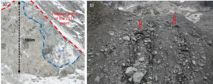
Figure S3: a) Rock fall release plane of the 2011 rock fall event. The right part of the release 401
plane is covered with blue permafrost ice b) Blowholes in 2017 deposits in Area 1a (red arrows). 402
Geyser-like water fountains were observed 25 to 40 minutes after the 2017 event from these 403 blowholes. 404 405 406 407 408 409
Figure S4: Map of seismic broadband stations near Pizzo Cengalo. 410
411 412
19 413
Figure S5: Three-component waveform fits (red dashed) to low-frequency seismic ground 414
displacement records (black) of the 2017 Pizzo Cengalo rock avalanche. Station distances to 415
rock avalanche and frequency ranges over which the inversion was applied and data were 416
filtered, are indicated. Data and fits are normalized to the strongest component of a given 417 station. 418 419 420 421 422 423 424 425
20 426
Figure S6: Rock avalanche trajectory. A: Same as Figure 7 of the main text, except for 427
additionally showing all jackknife trajectories (black lines). B: Three dimensional view of the 428
Bondasca Valley and the rock avalanche path (red) calculated from the mean of the jackknife 429
force histories. Note that the terrain step (Figures 1 and 2 in the main text), which the rock 430
avalanche encountered after more gently inclined terrain down-slope of the Bügeleisen 431
ridgeline, manifests itself in the trajectory. 432
433 434 435
21 436
Figure S7: Spectral signature of the 2017 event. (A) time series with discussed sections color 437
coded. (B) Spectrogram as in Figure 5 of the main text. Black vertical bars delimit the color 438
coded seismogram sections in Panel (A). (C) Normalized spectra of the color coded seismogram 439
sections in Panel (A). 440
441 442