Optimising the compilation of Petri net models

HAL Id: hal-00666661

https://hal.archives-ouvertes.fr/hal-00666661

Submitted on 29 Nov 2013

HAL is a multi-disciplinary open access

archive for the deposit and dissemination of

sci-entific research documents, whether they are

pub-lished or not. The documents may come from

teaching and research institutions in France or

abroad, or from public or private research centers.

L’archive ouverte pluridisciplinaire HAL, est

destinée au dépôt et à la diffusion de documents

scientifiques de niveau recherche, publiés ou non,

émanant des établissements d’enseignement et de

recherche français ou étrangers, des laboratoires

publics ou privés.

Lukasz Fronc, Franck Pommereau

To cite this version:

Lukasz Fronc, Franck Pommereau. Optimising the compilation of Petri net models. Second

In-ternational Workshop on Scalable and Usable Model Checking for Petri Net and other models of

Concurrency (SUMO 2011), Jun 2011, Kanazawa, Japan. pp.49–64. �hal-00666661�

Lukasz Fronc and Franck Pommereau

IBISC, University of ´Evry, Tour ´Evry 2 523 place des terrasses de l’Agora, 91000 ´Evry, France

{fronc,pommereau}@ibisc.univ-evry.fr

Abstract. Compilation of a Petri net model is one way to accelerate its analysis through state space exploration. In this approach, code to explore the Petri net states is generated, which avoids the use of a fixed exploration tool involving an interpretation of the Petri net structure. In this paper, we present a code generation framework for coloured Petri nets targeting various languages (Python, C and LLVM) and featuring optimisations based on peculiarities in models like places types, bound-edness, invariants, etc. When adequate modelling tools are used, these properties can be known by construction and we show that exploiting them does not introduce any additional cost while further optimising the generated code. The accelerations resulting from this optimised compi-lation are then evaluated on various Petri net models, showing speedups and execution times competing with state-of-the-art tools.

Keywords:explicit model-checking, acceleration, model compilation

1

Introduction

System verification through model-checking is one of the major research domains in computer science [3]. It consists in defining a formal model of the system to be analysed and then use an automated tool to check whether the expected properties are met or not. In this paper, we consider more particularly the do-main of coloured Petri nets [18], widely used for modelling, and the explicit model-checking approach that enumerates all the reachable states of a model (contrasting with symbolic model-checking that handles directly sets of states). Among the numerous techniques to speedup explicit model-checking, model compilation may be used to generate source code then compiled into machine code to produce a high-performance implementation of the state space explo-ration. For instance, this approach is successfully used by Helena [5, 24] that generates C code and the same approach is also used by the well-known model-checker Spin [16]. This accelerates computation by avoiding an interpretation of the model that is instead dispatched within a specially generated analyser.

The compilation approach can be further improved by exploiting peculiari-ties in the model of interest in order to optimise the generated code [19]. For instance, we will see in the paper how 1-boundedness of places may be exploited. Crucially, this information about the model can often be known by construction if adequate modelling techniques are used [27], avoiding any analysis before state

space exploration, which would reduce the overall efficiency of the approach. This differs from other optimisations (that can be also implemented at compile time) like transitions agglomeration implemented in Helena [6].

In this paper, we present a Petri net compiler infrastructure and consider simple optimisations, showing how they can accelerate state space computation. Theses optimisations are not fundamentally new and similar ideas can be found in Spin for example. However, to the best of our knowledge, this is the first time such optimisations are considered for coloured Petri nets. This allows us for in-stance to outperform the well-known tool Helena, often regarded as the most efficient explicit model-checker for coloured Petri nets. Moreover, our approach makes use of a flexible high-level programming language, Python, as the colour domain of Petri nets, which enables for quick and easy modelling. By exploiting place types provided in the model, most of Python code in the model can be actu-ally staticactu-ally typed, allowing to generate efficient machine code to implement it instead of resorting to Python interpretation. This results in a flexible modelling framework that is efficient at the same time, which are in general contradictory objectives. Exploiting a carefully chosen set of languages and technologies, our framework enables the modeller for using an incremental development process based on quick prototyping, profiling and optimisation.

The rest of the paper is organised as follows: we first recall the main no-tions about coloured Petri nets and show how they can be compiled into a set of algorithms and data structures dedicated to state space exploration. Then section 3 discusses basic optimisations of these elements and section 4 presents benchmarks to evaluate the resulting performances, including a comparison with Helena. For simplicity, we restrict our algorithms to the computation of reacha-bility sets, but they can be easily generalised to compute reachareacha-bility graphs.

2

Coloured Petri nets and their compilation

A (coloured) Petri net involves a colour domain that provides data values, vari-ables, operators, a syntax for expressions, possibly typing rules, etc. Usually, elaborated colour domains are used to ease modelling; in particular, one may consider a functional programming language [18, 29] or the functional fragment (expressions) of an imperative programming language [24, 26]. In this paper we will consider Python as a concrete colour domain. Concrete colour domains can be seen as implementations of a more general abstract colour domain providing D_{the set of data values, V the set of variables and E the set of expressions. Let} e ∈ E, we denote by vars(e) the set of variables from V involved in e. Moreover, variables or values may be considered as (simple) expressions, i.e., we assume D_{∪ V ⊆ E. At this abstract level, we do not make any assumption about the} typing or syntactical correctness of expressions; instead, we assume that any ex-pression can be evaluated, possibly to ⊥ /∈ D (undefined value) in case of any error. More precisely, a binding is a partial function β : V → D ∪ {⊥}. Then, let e ∈ E and β be a binding, we extend the application of β to denote by β(e) the evaluation of e under β; if the domain of β does not include vars(e) then

β(e)df

= ⊥. The evaluation of an expression under a binding is naturally extended to sets and multisets of expressions.

Definition 1 (Petri nets). A Petri net is a tuple (S, T, ℓ) where S is the finite set of places, T , disjoint from S, is the finite set of transitions, and ℓ is a labelling function such that:

– for all s ∈ S, ℓ(s) ⊆ D is the type of s, i.e., the values that s may contain; – for all t ∈ T , ℓ(t) ∈ E is the guard of t, i.e., a condition for its execution; – for all (x, y) ∈ (S × T ) ∪ (T × S), ℓ(x, y) is a multiset over E and defines the

arc from x toward y.

Amarking of a Petri net is a map that associates to each place s ∈ S a multiset of values from ℓ(s). From a marking M , a transition t can be fired using a binding β and yielding a new marking M′_{, which is denoted byM [t, βiM}′_{, iff:}

– there are enough tokens: for all s ∈ S, M (s) ≥ β(ℓ(s, t)); – the guard is validated: β(ℓ(t)) is true;

– place types are respected: for all s ∈ S, β(ℓ(t, s)) is a multiset over ℓ(s); – M′

is M with tokens consumed and produced according to the arcs: for all s ∈ S, M′_{(s) = M (s) − β(ℓ(s, t)) + β(ℓ(t, s)).}

Such a bindingβ is called a mode of t at marking M . For a Petri net nodex ∈ S ∪ T , we define•_xdf

= {y ∈ S ∪ T | ℓ(y, x) 6= ∅} and x•_{= {y ∈ S ∪ T | ℓ(x, y) 6= ∅} where ∅ is the empty multiset. Finally, we extend}df

the notation vars to a transition by taking the union of the variable sets in its guard and connected arcs.

In the rest of this section and in the next two sections, we consider a fixed Petri net N = (S, T, ℓ) to be compiled.df

2.1 Compilation of coloured Petri nets

In order to allow for translating a Petri net into a library, we need to make further assumptions about its annotations. First, we assume that the considered Petri net is such that, for all transition t ∈ T , and all s ∈ S, ℓ(s, t) is either empty or contains a single variable (i.e., ℓ(s, t) = {xs,t} ⊂ V). We also assume

that vars(t) = Ss∈Svars(ℓ(s, t)), i.e., all the variables involved in a transition

can be bound using input arcs. The second assumption is a classical one that allows to simplify the discovery of modes. The first assumption is made without loss of generality to simplify the presentation.

The following definition allows to relate the Petri net to be compiled to the chosen target language, assuming it defines notions of types (statical or dynamical) and functions (with parameters). We need to concretise place types and implement expressions.

– for all place s ∈ S, ℓ(s) is a type of the target language, interpreted as a subset of D;

– for all transition t ∈ T , ℓ(t) is a call to a Boolean function whose parameters are the elements of vars(t);

– for all s ∈ t•

,ℓ(t, s) can be evaluated calling a function ft,swhose parameters

are the elements of vars(t) and that returns a multiset over ℓ(s), i.e., ft,s is

equivalent to a single instruction “return ℓ(t, s)”; – all the functions involved in the annotations terminate.

Given an initial marking M0, we want to compute the set R of reachable

markings, i.e., the smallest set such that M0∈ R, and if M ∈ R and M [t, βiM′

then M′_{∈ R also. To achieve this computation, we compile the underlying Petri}

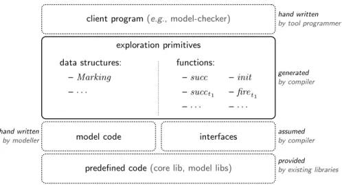
net into a library. The compilation process aims to avoid the use of a Petri net data structure by providing exploration primitives that are specific to the model. These primitives manipulate a unique data structure, Marking, that stores a state of the Petri net. The generated library will be used by a client program, a model-checker or a simulator for instance, and used to explore the state space. Thus, it has to respect a fixed API to ensure a correct interfacing with the client program. Moreover, the library relies on primitives (like an implementation of sets) that are assumed to be predefined, as well as code directly taken from the compiled model. This structure is presented in figure 1.

The compiled library is formed of two main parts, data structures which contain the marking structure plus auxiliary structures, and functions for state space exploration. The marking structure is generated following peculiarities of

client program(e.g., model-checker)

model code interfaces

predefined code(core lib, model libs)

exploration primitives data structures: – Marking –· · · functions: – succ – succt1 –· · · – init – firet1 –· · · hand written by tool programmer generated by compiler assumed by compiler provided by existing libraries hand written by modeller

Fig. 1.The compiler generates a library (data structures and functions) that is used by a client program (e.g., a model-checker or a simulator) to explore the state space. This library uses code from the model (i.e., Petri nets annotations) as well as existing data structures (e.g., sets and multisets) forming a core libraries, and accesses them through normalised interfaces. Model code itself may use existing code but it is not expected to do it through any particular interface.

the Petri net in order to produce an efficient data structure. This may include fully generated components or reuse generic ones, the latter have been hand-written and forms a core library that can be reused by the compiler. To make this reusing possible as well as to allow for using alternative implementations of generic components, we have defined a set of interfaces that each generic component implementation has to respect.

A firing function is generated for each transition t to implement the successor relation M [t, βiM′_{: given M and the valuation corresponding to β, it computes}

M′_{. A successor function succ}

tis also generated for each transition t to compute

{M′_{| M [t, βiM}′_{} given a marking M . More precisely, this function searches for}

all modes at the given marking and produces the set resulting from the corre-sponding firing function calls. We also produce a function init that returns the initial marking of the Petri net, and a global successor function succ that com-putes {M′ _{| M [t, βiM}′

, t ∈ T } given a marking M , and thus calls all the transi-tion specific successor functransi-tions. These algorithms are presented in the following.

Let t ∈ T be a transition such that•_{t = {s}

1, . . . , sn} and t•= {s′1, . . . , s ′ m}.

Then, the transition firing function firetcan be written as shown in figure 2. This

function simply creates a copy M′ _{of M , removes from it the consumed tokens}

(xt,s1, . . . , xt,sn) and adds the produced ones before to return M

′_{. One could}

remark that it avoids a loop over the Petri net places but instead it executes a sequence of statements. Indeed, this is more efficient (no branching penalties, no loop overhead, no array for the functions ft,s′

j, . . . ) and the resulting code is

simpler to produce. It is important to notice that we do not need a data structure for the modes. Indeed, for each transition t we use a fixed order on •_{t, which}

allows to implicitly represent a mode though function parameters and avoids data structure allocation and queries.

The algorithm to compute the successors of a marking through a transition enumerates all the combinations of tokens from the input places. If a combination validates the guard then the suitable transition firing function is called and produce a new marking. This is shown in figure 3. The nesting of loops avoids an iteration over•_{t, which saves from querying the Petri net structure and avoids}

the explicit construction of a binding. Moreover, like ft,s′jabove, gtis embedded

in the generated code instead of being interpreted.

The global successor function succ returns the set of all the successors of a marking by calling all transition specific successor functions and accumulating the discovered markings into the same set. This is shown in figure 4.

2.2 Structure of our compilation framework

Our compilation framework comprises a frontend part that translate a Petri net model into an abstract representation of the target library (including abstracted algorithms and data structures). This representation is then optimised exploiting Petri net peculiarities. For each target language, a dedicated backend is respon-sible for translating the abstract representation into code in the target language, and integrate the result with existing components from the core library as well as with the code embedded within the Petri net annotations.

fire_t: M, xt,s1, . . . , xt,sn→ M ′

M′_{← copy(M ) // copy marking M}

M′_(s 1) ← M′(s1) − {xt,s1} // consume tokens · · · M′_(s n) ← M′(sn) − {xt,sn} M′_(s′ 1) ← M′(s′1) + ft,s′ 1(xt,s1, . . . , xt,sn) // produce tokens · · · M′_(s′ m) ← M′(s′m) + ft,s′_m(xt,s1, . . . , xt,sn) returnM′ _{// return the successor marking}

Fig. 2.Transition firing algorithm.

succt: M, next → ⊥

forxt,sn inM (sn) do // enumerate place sn · · ·

forxt,s1 inM (s1) do // enumerate place s1

if gt(xt,s1, . . . , xt,sn) then // guard check

next← next ∪ {firet(M, xt,s1, . . . , xt,sn)} // add a successor marking endif

endfor · · · endfor

Fig. 3.Transition specific successors computation algorithm.

succ: M → next next← ∅ succt1(M , next) succt2(M , next) · · · succtn(M , next) returnnext

Fig. 4.Computation of a marking successors.

We currently have implemented three backends targeting respectively Python, Cython and LLVM languages. Python is a well-known high-level, dynamically typed, interpreted language [28] that is nowadays widely used for scientific com-puting [23]. Cython is an extension of Python with types annotations, which allows Cython code to be compiled into efficient C code, thus removing most of the overheads introduced by the Python interpretation [1]. The resulting C code is then compiled to a library that can be loaded as a Python module or from any program in a C-compatible language. The Cython backend is thus also a C backend. LLVM is a compiler infrastructure that features a high-level, machine-independent, intermediate representation that can be seen as a typed assembly

Petri net model peculiarities structure annotations frontend abstract code compiler optimisers backend core lib code generator target code

Fig. 5.Structure of the compilation framework.

language [21]. This LLVM code can be executed using a just-in-time compiler or compiled to machine code on every platform supported by the LLVM project.

We consider Petri nets models using Python as their colour domain. The compatibility with the Python and Cython backends is thus straightforward. In order to implement the LLVM backend, we reuse the Cython backend to generate a stripped down version of the target library including only the annotations from the model. This simplified library is then compiled by Cython into C code that can be handled by the LLVM toolchain.

3

Optimisations guided by Petri net structures

In this section, we introduces different kinds of optimisations that are indepen-dent and can be applied separately or simultaneously.

3.1 Statically typing a dynamically typed colour domain

This optimisation aims at statically typing the Python code embedded in a Petri net model. In this setting, place types are specified as Python classes among which some are built-in primitive types (e.g., int, str , bool , etc.) actually imple-mented in C. The idea is to use place types to discover the types of variables, choosing the universal type (object in Python) when a non-primitive type is found. When all the variables involved in the computation of a Python expres-sion can be typed with primitive types, the Cython compiler produces for it an efficient C implementation, without resorting to the Python interpreter. This results in an efficient pure C implementation of a Python function, similar to the primitive functions already embedded in Python.

In the benchmarks presented in the next section, this optimisation is always turned on. Indeed, without it, the generated code runs at the speed of the Python interpreter, that may dramatically slower, especially when most of data can be statically typed to primitive types (see section 4.3).

3.2 Implementing a known optimisation

Each function succtenumerates the variables from the input arcs in an arbitrary

order. The order of the loops thus has no incidence on the algorithm correction, but it can produce an important speedup as shown in [8]. For instance, consider two places s1, s2 ∈ •t. If we know that s1 is 1-bounded but not s2, then it is

more efficient to enumerate tokens in s1 before those in s2 because the former

enumeration is cheaper than the latter and thus we can iterate on s2 only if

necessary. More generally, the optimisation consists in choosing an ordering of the input arcs to enumerate first the tokens from places with a lower boundary or a type with a smaller domain. The optimisation presented in [8] is actually more general and also relies on observations about the order in which variables are bound, which is off-topic in our case considering the restrictions we have imposed on input arcs and guard parameters. However, in the more general setting of our implementation, we are using the full optimisation as described in [8].

In general, place-bounds for an arbitrary Petri net are usually discovered by computing the state space or place invariants [14, 17]. However, using ade-quate modelling tools or formalisms, this property may be known by construction for many places: in particular, control-flow places in algebras of coloured Petri nets [27] can be guaranteed to be 1-bounded by construction.

3.3 Exploiting 1-bounded places

Let M be a marking and assume a place sk ∈•t that is 1-bounded. In such a

case, we can replace the kth_{“for” loop by an “if ” block in the t-specific successor}

algorithm. Indeed, we know that sk may contain at most one token and so,

iterating over M (sk) is equivalent to check whether sk is not empty and then

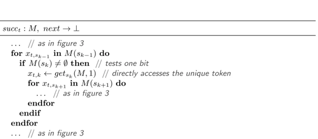
retrieve its unique token. This is shown in figure 6, combined with the following optimisation.

3.4 Efficient implementations of places

This optimisation consists in replacing a data structure by another one but preserving the interfaces. As a first example, let us consider a 1-bounded place of type {•}. This is the case for instance for control-flow places in algebras of coloured Petri nets [27]. The optimisation consists in replacing the generic data structure for multisets by a much more efficient implementation storing only a Boolean value (i.e., one bit) to indicate whether the place is marked or not.

Similarly, a 1-bounded coloured place may be implemented using a single value to store a token value together with a Boolean to know whether a token is actually present or not. (Another implementation could use a pointer to the token value that would be null whenever the place is empty, but this version suffers from the penalty of dynamic memory management.) An example is given in figure 6 in conjunction with the optimisation from section 3.3.

Finally, a place whose type is bool may be implemented as a pair of counters to store the number of occurrences of each Boolean value present in the place.

succt: M, next → ⊥

. . . // as in figure 3

forxt,s_k−1 inM (sk−1) do

if M (sk) 6= ∅ then // tests one bit

xt,k← getsk(M, 1) // directly accesses the unique token forxt,sk+1 inM (sk+1) do . . . // as in figure 3 endfor endif endfor . . . // as in figure 3

Fig. 6. An optimisation of the algorithm presented in figure 3 where function

gets_k(M, i) returns the i-th token in the domain of M (sk).

This is likely to be more efficient than a hashtable-based implementation and may be generalised to most types with a small domain.

4

Experimental results

The compilation approach presented in this paper is currently being imple-mented. We use a mixture of different programming languages: LLVM, C, Python and Cython (both to generate C from Python, and as a glue language to inter-face all the others). More precisely, we use the SNAKES toolkit [25, 26], a library for quickly prototyping Petri net tools, it is used here to import Petri nets and explore their structure. We also use LLVM-Py [22], a Python binding of the LLVM library to write LLVM programs in a “programmatic” way, i.e., avoiding to directly handle source code. It is used here to generate all the LLVM code for state space algorithms. Finally, the core library is implemented using either Python, Cython, LLVM and C. For instance, we directly reuse the efficient sets implementation built into Python, multisets are hand-written in Cython on the top of Python dictionaries (based on hash tables) and a few auxiliary data struc-tures are hand-written directly in C or LLVM. All these language can be mixed smoothly because they are all compatible with C (Python itself is implemented in C and its internal API is fully accessible). The compiler is fully implemented in Python, which is largely efficient enough as shown by our experiments below. As explained already, the compilation process starts with the front-end that analyses the Petri net and produces an abstract representation (AR) of the algorithms and data structures to be generated. Algorithmic optimisations are performed by the front-end directly on the AR. Then, depending on the selected target language, a dedicated backend is invoked to generate and compile the target code. Further optimisations on data-structure implementation are actually performed during this stage. To integrate these generated code with predefined data structures, additional glue code is generated by the backend. The result

is a dynamic library that can be loaded from the Python interpreter as well as called from a C or LLVM program.

The rest of the section presents three case studies allowing to demonstrate the speedups introduced by the optimisations presented above. The machine used for benchmarks was a standard laptop PC equipped with an Intel i5-520M processor (2.4GHz, 3MB, Dual Core) and 4GB of RAM (2x2GB, 1333MHz DDR3) with virtual memory swapping disabled. We compare our implemen-tation with Helena (version 1.5) and focus on three main aspects of computa-tion: total execution time, model compilation time and state space search time. Each reported measure is expressed in seconds and was obtained as the aver-age of ten independent runs. Finally, in order to ensure that both tools use the same model and compute the same state space, static reduction were disabled in Helena. In order to generate the state space, a trivial client program was produced to systematically explore and store all the successors of all reached markings. All the presented results are obtained using the Cython backend that is presently the most efficient of our three backends, and is as expressive as Python. All the files and programs used for these benchmarks may be obtained at hhttp://www.ibisc.fr/~lfronc/SUMO-2011i.

4.1 Dinning Philosophers

The first test case consists in computing the state space of a Petri net model of the Dinning Philosophers problem, borrowed from [4]. The considered Petri is a 1-bounded P/T net so we use the corresponding optimisation discussed above. The results for different numbers of philosophers are presented in table 1. We can observe that our implementation is always more efficient than Helena and that the optimisations introduce a notable speedup with improved compilation times (indeed, optimisation actually simplifies things). In particular, we would like to stress that the compilation time is very satisfactory, which validates the fact that it is not crucial to optimise the compiler itself.

We also observe that without optimisations our library cannot compute the state space for more than 33 philosophers, and with the optimisations turned on, it can reach up to 36 philosophers. Helena can reach up to 37 philosophers but fails with 38, which can be explained by its use of a state space compression technique that stores about only one out of twenty states [5, 9]. The main conclu-sion we draw from this example is that our implementation is much faster than Helena on P/T nets, even without optimisations and that compilation times are much shorter. We observe also that it is also more efficient on bigger state spaces (cases 35 and 36). Following [15], we believe that this is mainly due to avoidance of hash clashes and state comparison when storing states, which validates the efficiency of the model-specific hash functions we generate.

4.2 A railroad crossing model

This test case is a model of a railroad crossing system, that generalises the simpler one presented in [27, sec. 3.3] to an arbitrary number of tracks. This

n states not optimised optimised speedup Helena speedup t c s t c s t c s 24 103 682 4,7 3,8 0,9 2,4 1,8 0,6 2,0 14,7 12,1 2,6 6,2 25 167 761 5,7 4,0 1,6 3,0 1,8 1,2 1,9 17,5 13,0 4,5 5,8 26 271 443 7,0 4,1 3,0 4,1 1,9 2,2 1,7 20,8 13,0 7,8 5,1 27 439 204 9,6 4,3 5,3 5,9 1,9 4,0 1,6 27,5 14,0 13,5 4,7 28 710 647 14,0 4,8 9,2 9,0 2,0 7,0 1,6 39,1 14,0 25,1 4,3 29 1 149 851 20,9 4,8 16,1 14,9 2,1 12,8 1,4 57,7 15,0 42,7 3,9 30 1 860 498 34,3 5,0 29,3 24,5 2,1 22,4 1,4 92,5 15,0 77,5 3,8 31 3 010 349 56,6 5,4 51,2 41,2 2,1 39,1 1,4 158,0 16,0 142,0 3,8 32 4 870 847 92,8 5,7 87,1 69,8 2,2 67,6 1,3 277,5 16,0 261,5 4,0 33 7 881 196 155,7 6,0 149,8 114,2 2,3 111,9 1,4 437,1 17,0 420,1 3,8 34 12 752 043 - - - 193,4 2,3 191,1 - 860,1 17,0 843,1 4,4 35 20 633 239 - - - 345.1 2.4 342.7 - 1905.7 18.5 1887.2 5.5 36 33 385 282 - - - 598.9 2.4 596.5 - 4253.8 18.5 4235.3 7.1 37 54 018 521 - - - 10217 19.0 10198.1

-Table 1. Performance tests based on n philosophers, where t is the total execution time, s is the total state space search time and c is the compilation time. The left-most column entitled “speedup” corresponds to the total time in the unoptimised model divided by the total time in the optimised model. The right-most “speedup” column is the total time spent by Helena divided by the total time in the optimised model.

n states not optimised optimised speedup Helena speedup

t c s t c s t c s 7 30 626 3.7 3.5 0.2 2.2 2.1 0.2 1.6 14.4 14.0 0.4 6.4 8 124 562 5.1 3.9 1.2 3.1 2.2 0.9 1.6 17.4 15.0 2.4 5.6 9 504 662 10.6 4.3 6.3 6.7 2.4 4.3 1.6 28.9 17.0 11.9 4.3 10 2 038 166 33.9 4.8 29.1 23.8 2.6 21.3 1.4 73.0 18.0 55.0 3.1 11 8 211 530 140.7 5.2 135.5 108.5 2.8 105.7 1.3 345.0 20.0 325.0 3.2 12 33 023 066 - - - 2721.6 23.0 2698.6

-Table 2.Performance tests based on n tracks of the railroad model, where t, s, c and “speedup” are as in table 1.

system comprises a gate, a set of tracks equipped with green lights, as well as a controller to count trains and command the gates accordingly. For n tracks, this Petri net has 5n + 11 black-token 1-bounded places (control flow or flags), 2 typed 1-bounded places (counter of trains and gate position), 3 integer-typed colour-safe places (tracks green lights) and 1 black-token n-bounded place (signals from track to controller). The benchmarks results are shown in table 2. As above, we notice that our implementation is faster than Helena even without optimisations, and that the optimisations result in similar speedups. We could compute the state space for at most 11 tracks while Helena can reach 12 tracks but fails at 13.

not optimised optimised speedupexploration t c s t c s speedup with Python 5.00 0.07 4.93 4.18 0.07 4.11 1.20 1.20 attacker Cython 5.50 2.36 3.14 4.83 2.02 2.82 1.14 1.11 without Python 2.58 0.07 2.51 1.85 0.07 1.78 1.40 1.41 attacker Cython 3.32 2.36 0.97 2.79 2.02 0.77 1.19 1.26

Table 3.Computation of the state space of the security protocol model, where t, s, c and “speedup” columns are as in table 1.

3 4 5 6 7 0 2 4 6 8 10 12 not optimised optimised

Cython faster than Python Cython slower than Python

117,649 states

n = 6 not optimised optimised speedup

Python 403.9 109.1 3.7

Cython 37.4 29.2 1.3

Fig. 7.Speedup of Cython compared with Python for n sessions of the protocol.

4.3 Security protocol model

The last test case is a model of the Needham-Schroeder public key cryptographic protocol, borrowed from [13]. It embeds about 350 lines of Python code to im-plement the learning algorithm of a Dolev-Yao attacker. This model comprises 17 places optimised as discussed above whenever possible: 11 are black-token bounded places to implement the control-flow of agents; 6 are coloured 1-bounded places to store the agents’ knowledge; 1 is an un1-bounded coloured place to store the attacker’s knowledge. Coloured tokens are Python objects or tuples of Python objects. Such a Petri net structure is typical for models of cryptographic protocols like those considered in [13].

For this example, it is not possible to draw a direct comparison with Helena since there is no possible translation of the Python part of the model into the language embedded in Helena. However, compared with a Helena model of the same protocol from [2], we observe equivalent execution times for a SNAKES-based exhaustive simulation and a Helena run. The state space exploration is much faster using Helena but its compilation time is very long (SNAKES does not compile). In our current experiment, we can observe that the compilation time is as good as with other models because the annotations in this model are Python expressions that can be directly copied to the generated code, while Helena needs to translate the annotation of its Petri net model into C code.

have first presented the whole execution times, then when have excluded the time spent in the Dolev-Yao attacker algorithms that is user-defined external code that no Petri net compiler could optimise. This allows to extract a more relevant speedup that is similar with the previous tests. However, one could observe that the Python version outperforms the Cython version and executes faster and with better speedups. This is actually due to the small size of the state space (only 1234 states), which has two consequences. First, it gives more weight to the compilation time: the Python backend only needs to produce code, whereas the Cython backend also calls Cython and a C compiler. Second, the benefits from Cython can be better observed on the long run because it optimises loops in particular. This is indeed shown in figure 7 that depicts the speedups obtained by compiling to Cython instead of Python with respect to the number of parallel session of the Needham-Schroeder protocol without attacker. To provide an order of magnitude, we have also shown the number of states for 6 sessions and the speedups obtained from the optimisations. This also allows to observe that our optimisations perform very well on Python also and reduce the execution times, which in turn reduces benefits of using Cython. This is not true in general but holds specially on this model that comprises many Python objects that cannot be translated to C efficient code. So, the Cython code suffers from many context switching between C and Python parts.

We would like to note also that the modelling time and effort is much larger when developing a model using the language embedded in Helena rather than using a full-featured language like Python. So, there exists a trade-off between modelling, compilation and verification times that is worth considering. This is why we consider as crucial for our compiler to enable the modeller for quick prototyping with incremental optimisation, as explained in [1]. In our case, the Python implementation of the attacker may be compiled using Cython and op-timised by typing critical parts (i.e., main loops). Compared with the imple-mentation of the Dolev-Yao attacker using Helena colour language from [2], the Python implementation we have used is algorithmically better because it could use Python efficient hash-based data structures (sets and dictionaries) while He-lena only offers sequential data structures (arrays and lists), which is another argument in favour of using a full-featured colour language.

As a conclusion about performances for this test case, let us sum up inter-esting facts: SNAKES and Helena version run in comparable times, the latter spends much more time in compilation but the former has more efficient data structures; our compilation is very efficient; our Python backend is typically 10 times faster than SNAKES simulation; our Cython backend is typically 2 to 4 times faster than the Python backend. So we could reasonably expect very good performances on a direct comparison with Helena.

5

Conclusion

We have shown how a coloured Petri net can be compiled to produce a library that provides primitives to compute the state space. Then, we have shown how

different kinds of optimisations can be considered, taking into account peculiari-ties in the model. We have considered places types and boundaries in particular. Finally, our experiments have demonstrated the relevance of the approach, show-ing both the benefits of the optimisations (up to almost 2 times faster) and the overall performance with respect to the state-of-the-art tool Helena (up to 7 times faster). Moreover, we have shown that a well chosen mixture of high- and low-level programming languages enables the modeller for quick prototyping with incremental optimisation, which allows to obtain results with reduced time and efforts. Our comparison with Helena also showed that our compilation process is much faster in every case (around 7 times faster). Our optimisations rely on model-specific properties, like place types and boundaries, and do not introduce additional compilation time, instead optimisation may actually simplifies things and fasten compilation.

The idea of exploiting models properties has been defended in [27] and suc-cessfully applied to the development of a massively parallel state space explo-ration algorithm for Petri net models of security protocols [13], or in [20] to reduce the state space of models of multi-threaded systems. Let us also remark that the LLVM implementation of the algorithms and code transformations (i.e., optimisations) presented in this paper has been formally proved in [11, 12], which is an important aspect when it comes to perform verification. Crucially, these proofs rely on our careful modular design using fixed and formalised interfaces between components.

Our current work is focused toward finalising our compiler, and then in-troducing more optimisations. In particular, we would like to improve memory consumption by introducing memory sharing, and to exploit more efficiently the control flow places from models specified using algebras of Petri nets [27]. In par-allel, we will develop more case studies to assess the efficiency of our approach. We are also investigating a replacement of the Helena compilation engine with ours, allowing to bring our performances and flexible modelling environment to Helena while taking advantage of its infrastructure, in particular the memory management strategies [7, 9, 10] and the static Petri nets reductions [6].

References

1. S. Behnel, R. Bradshaw, C. Citro, L. Dalcin, D. Seljebotn, and K. Smith. Cython: The best of both worlds. Computing in Science & Engineering, 13(2), 2011. 2. R. Bouroulet, H. Klaudel, and E. Pelz. Modelling and verification of authentication

using enhanced net semantics of SPL (Security Protocol Language). In ACSD’06. IEEE Computer Society, 2006.

3. E. Clarke, A. Emerson, and J. Sifakis. Model checking: Algorithmic verification and debugging. ACM Turing Award, 2007.

4. R. Esser. Dining philosophers Petri net. hhttp://goo.gl/jOFh5i, 1998.

5. S. Evangelista. M´ethodes et outils de v´erification pour les r´eseaux de Petri de haut

niveau. PhD thesis, CNAM, Paris, France, 2006.

6. S. Evangelista, S. Haddad, and J.-F. Pradat-Peyre. Syntactical colored Petri nets reductions. In ATVA’05, volume 3707 of LNCS. Springer, 2005.

7. S. Evangelista and L. Kristensen. Search-order independent state caching.

ToP-NOC III, to appear, 2010.

8. S. Evangelista and J.-F. Pradat-Peyre. An efficient algorithm for the enabling test of colored Petri nets. In CPN’04, number 570 in DAIMI report PB. University of ˚

Arhus, Denmark, 2004.

9. S. Evangelista and J.-F. Pradat-Peyre. Memory efficient state space storage in explicit software model checking. In SPIN’05, volume 3639 of LNCS. Springer, 2005.

10. S. Evangelista, M. Westergaard, and L. Kristensen. The ComBack method revis-ited: caching strategies and extension with delayed duplicate detection. ToPNOC

III, 5800:189–215, 2009.

11. L. Fronc. Analyse efficace des r´eseaux de Petri par des techniques de compilation. Master’s thesis, MPRI, university of Paris 7, 2010.

12. L. Fronc and F. Pommereau. Proving a Petri net model-checker implementation. Technical report, IBISC, 2011. Submitted paper.

13. F. Gava, M. Guedj, and F. Pommereau. A BSP algorithm for the state space construction of security protocols. In PDMC’10. IEEE Computer Society, 2010. 14. H. Genrich and K. Lautenbach. S-invariance in predicate/transition nets. In

Eu-ropean Workshop on Applications and Theory of Petri Nets, 1982.

15. G. Holzmann. An improved protocol reachability analysis technique. Software,

Practice and Experience, 18(2), 1988.

16. G. Holzmann and al. Spin, formal verification. hhttp://spinroot.comi.

17. K. J. Coloured Petri nets and the invariant-method. Theoretical Computer Science, 14(3), 1981.

18. K. Jensen and L. Kristensen. Coloured Petri Nets: Modelling and Validation of

Concurrent Systems. Springer, 2009, ISBN 978-3-642-00283-0.

19. R. Jourdier. Compilation de r´eseaux de Petri color´es. Master’s thesis, University of ´Evry, 2009.

20. H. Klaudel, M. Koutny, E. Pelz, and F. Pommereau. State space reduction for dynamic process creation. Scientific Annals of Computer Science, 20, 2010. 21. C. Lattner and al. The LLVM compiler infrastructure. hhttp://llvm.orgi. 22. R. Mahadevan. Python bindings for LLVM. hhttp://www.mdevan.org/llvm-pyi. 23. K. Millman and M. Aivazis, editors. Python for Scientists and Engineers, volume

13(2) of Computing in Science & Engineering. IEEE Computer Society, 2011. 24. C. Pajault and S. Evangelista. Helena: a high level net analyzer. hhttp://helena.

cnam.fri.

25. F. Pommereau. SNAKES is the net algebra kit for editors and simulators. hhttp: //www.ibisc.univ-evry.fr/~fpommereau/snakes.htmi.

26. F. Pommereau. Quickly prototyping Petri nets tools with SNAKES. Petri net

newsletter, 2008.

27. F. Pommereau. Algebras of coloured Petri nets. LAMBERT Academic Publishing, October 2010, ISBN 978-3-8433-6113-2.

28. Python Software Foundation. Python programming language. hhttp://www. python.orgi.

29. C. Reinke. Haskell-coloured Petri nets. In IFL’99, volume 1868 of LNCS. Springer, 1999.