COPPER SPECIATION IN ESTUARIES AND COASTAL WATERS
by
Megan Brook Kogut B.S. Chemistry University of Washington
(1995)
M.S. Civil and Environmental Engineering
Massachusetts Institute of Technology (2000)
Submitted to the Department of Civil and Environmental Engineering in Partial Fulfillment of the Requirements for the Degree of
DOCTOR OF PHILOSOPHY In Environmental Chemistry
at the
Massachusetts Institute of Technology September 2002
@Massachusetts Institute of Technology
All rights reserved.
BkAKER MASSACHUSETTS WSTITUTC" OF TECHNOLOGY
SjEP 1 9j
LIBRARIES Signature of Author_ Department of Civil Certified byAssistant Professor, Civil
and Environmental Engineering
13 June 2002
Bettina Voelker and Environmental Engineering Thesis Supervisor
Accepted by 0 .... .
Oral Buyukozturk Chairman, Departmental Committee on Graduate Students
Cu speciation in estuaries and coastal waters
By Megan B. KogutSubmitted to the Department of Civil and Environmental Engineering On June 13, 2002 in Partial Fulfillment of the
Requirements for the Degree of Doctor of Philosophy in Environmental Chemistry
Abstract.
The goals of this dissertation are to better understand the sources and the Cu binding ability of ligands that control Cu toxicity in estuaries and harbors, where elevated Cu concentrations have caused documented toxic effects on microorganisms, fish, and benthic fauna. I modified and improved a commonly used approach to determine metal speciation (competitive ligand exchange adsorptive cathodic stripping voltammetry,
CLE-ACSV). Using this new approach to chemical Cu speciation and an old approach to
physical Cu speciation (filtration), I show that riverine humic substances, filtrable, recalcitrant and light absorbing molecules from degraded plant material, can account for all of the Cu binding in the Saco River estuary. This finding directly supports the hypothesis that terrestrial humic substances might be the most important source of Cu ligands for buffering Cu toxicity in coastal locations with freshwater inputs. However, fieldwork in coastal waters with large inputs of both Cu and suspended colloids (Boston Harbor, Narragansett Bay, and two ponds on Cape Cod) shows that some Cu present in these samples is inert to our competitive ligand exchange method for at least 48 hours. These results support the hypothesis that a significant fraction of the Cu present in these samples is physically sequestered in colloidal material, with the remaining fraction complexed by humic substances. Previous studies of Cu speciation were not able to distinguish between strongly complexed Cu and inert Cu, and our analytical approach should be used further to determine the role of colloids in Cu speciation in all natural waters.
Thesis Supervisor: Bettina M. Voelker
Acknowledgements.
I thank Tina Voelker for her tireless and instructive edits of this dissertation and for a
top-notch graduate student experience. Also I thank Jim Moffett for sharing his CSV tips and Harry Hemond for crucial support and encouragement.
I gratefully acknowledge those who provided necessary day-to-day laboratory support
and mental assistance: John MacFarlane, Mike Pullin, Jim Gawel, Nicole Keon, Alex Worden, Dave Senn, Daniel Collins, Greg Noonan, Rainer Lohmann, and Barbara Southworth.
I thank Shana Sturla and Nani Hunjan for exercising and feeding me while I was at MIT. I thank Jarred Swalwell for moving to Boston and supplying me with cheer and beer for
the last two years of my studies. Finally, I thank Gail Kogut, who sent me frequent fan email and who cheerfully rowed me back to the boat ramp when the outboard batteries died the second time on the Saco River.
Table of Contents.
Abstract. ... 1
Acknowledgem ents... 2
Chapter 1. Introduction ... 6
Chapter 2. Calibration of salicylaldoxime for pH and salinity... 10
2.1. Introduction... 10
2.2. M ethods ... 12
2.2.1. Relationships between pH, salinity and "true" stability constants of SA. 12 2.2.2. Calibration of SA for pH ... 15
2.2.3. M easurement of SRC(SA) ... 16
2.2.4. Calculation of KCuEDTA- - - - --... 17
2.2.5. Experimental setup. ... 17
2.2.6. Voltam m etric analyses... 18
2.3. Results... 18
2.3.1. SRC(SA) and salinity... 18
2.3.2. Cu-SA mono and bis speciation... 19
2.3.3. Calibration of SRC(SA) for variation in pH . ... 20
2.3.4. Ionic strength ... 22
2.4. Conclusions... 23
References. ... 25
Chapter 3. The contribution of riverine Cu ligands to Cu speciation in the Saco River estuary ... 33
Abstract ... 33
3.1. Introduction... 33
3.2. M ethods ... 37
3.2.1. Sam ple Collection... 37
3.2.2. Reagents ... 38
3.2.3. Filtering ... 38
3.2.4. Total organic carbon and color... 39
3.2.5. Total Cu... 39
3.2.6. CLE-ACSV ... 39
3.2.7. Setup for Cu overload and speciation titrations. ... 41
3.2.8. Cu speciation titrations... 42
3.3.2. Cu binding ability of riverine ligands with changes in pH and salinity.... 44
3.3.3. The binding ability of riverine ligands diluted to S=27%c ... 45
3.3.4. Internal calibration... 45
3.4. Discussion ... 46
3.4.1. Internal calibration... 46
3.4.2. Total organic carbon and color... 47
3.4.3. Riverine ligands... 48
3.4.4. Hum ic substances and the Saco riverine ligands... 48
3.5. Conclusions... 53
References . ... 54
Chapter 4. Kinetically inert Cu in coastal waters ... 66
Abstract. ... 66
4.1. Introduction... 67
4.2. M ethods ... 71
4.2.1. Sample Collection... 71
4.2.2. Filtration of Cu speciation samples ... 72
4.2.3. Dissolved organic m atter and salinity... 73
4.2.4. CLE-ACSV ... 73
4.2.5. Overload titration... 74
4.2.6. Total Cu... 76
4.2.7. Exchangeable and non-exchangeable Cu after 48 hours ... 77
4.2.8. Cu speciation titrations... 77
4.2.9. General titration setup ... 78
4.2.10.y ... 79
4.2.11. M odeling Cu speciation with FITEQL ... 80
4.3. Results... 81
4.3.1. Cu speciation ... 81
4.3.2. Internal calibrations and ligand "best fits"... 83
4.3.3. Filtration... 84
4.4. Discussion ... 85
4.4.1. Kinetically inert Cu... 85
4.4.2. Exchangeable ligands... 90
4.5. Conclusions... 92
References ... 94
Chapter 5. Cu Speciation in the Taunton River W atershed ... 108
5.1.2. POTW effluent as source of Cu... 109
5.1.3. Sewage as source of Cu ligands ... 109
5.1.4. Goals of Research ... 110
5.2. M ethods. ... 110
5.2.1. Site description ... 110
5.2.2. Sample collection... 111
5.2.3. W ater m ass balance for the Town River ... 112
5.2.4. M aterials... 113
5.2.5. CLE-ACSV ... 114
5.2.6. Calibration of ACSV with the overload titration... 116
5.2.7. Cu titration setup with overload titrations... 118
5.2.8. Calibration of sensitivity with addition of EDTA ... 118
5.2.9. Cu titration setup with EDTA calibration titrations ... 121
5.2.10. Determ ination of [Cu]T ... 122
5.2.11. Voltam m etric Analysis ... 122
5.3. Results and Discussion ... 123
5.3.1. Total and dissolved Cu... 123
5.3.2. Cu speciation titrations calibrated with overload titrations... 124
5.3.3. EDTA calibration... 127
5.4. Conclusions... 130
References. ... 132
Appendix A . The Conditional Stability Constant of CuEDTA2 ... ... .... ... .... 143
A. 1 Cu-EDTA Complexes... 143
A .2. Ionic Strength ... 144
A .3. Com petition of other cations with Cu for EDTA ... 145
A .4. Results... 146
References. ... 148
Appendix B. Approximation of the partitioning of salicylaldoxime into dissolved natural organic m atter. ... 151
B.1. Introduction. ... 151
B.2. Calculation of K0W for salicylaldoxim e... 153
References. ... 155
Appendix C. Correction factors for CLE-ACSV at different values of salinity and pH 158 Appendix D. Strong copper-binding behavior of terrestrial humic substances in seawater.
Chapter 1. Introduction
The toxicity of high concentrations of Cu to microorganisms and other species is of concern in polluted estuaries and nearshore waters. The toxicity of Cu is related to the concentration of free Cu, [Cu 2 ], and not to the concentration of total Cu. Cu is
distributed amongst the "free" form (usually <1% of total Cu) and Cu ligands (>99%), so that ligands control Cu toxicity. The goals of the work in this dissertation are to better understand sources and the Cu binding ability of ligands that control Cu toxicity in
streams and harbors, where elevated Cu concentrations have caused documented toxic effects on microorganisms, fish, and benthic fauna.
Using competitive ligand exchange adsorptive cathodic stripping voltammetry
(CLE-ACSV), I conducted field work that directly supports our hypothesis that terrestrial humic
substances are important Cu ligands in coastal locations with freshwater inputs. Our previously published work (Appendix D) shows that terrestrial humic substances, dissolved, recalcitrant and light absorbing molecules from degraded plant material, bind Cu strongly enough in seawater to possibly account for much of the Cu binding in near-shore areas. This work suggested that terrestrial humic substances might account most or all of the Cu binding in estuarine and coastal samples. We now show in Chapter 3 that the ligands in the Saco River can account for all of the Cu binding in a sample at high salinity (27%c) further downstream in the estuary. The binding ability of the Saco riverine ligands in the 27%o sample can be modeled as that of a very reasonable concentration of humic acid extract.
We also show that the binding ability of humic substances strongly depends on pH and salinity, but the pH dependence decreases with increasing salinity, which makes it
difficult to understand the effects of pH and salinity on riverine ligands. Therefore it will be difficult to predict the contribution of terrestrial humic substances to Cu binding in estuarine samples without investigating directly the change in their binding behavior upon mixing with seawater.
Also Chapter 3, I show in actual coastal field samples that the new calibration method we developed for CLE-ACSV (Appendix D) is needed to accurately measure the Cu binding ability of humic substances and therefore of field samples containing humic substances or any mixture of stronger and weaker Cu ligands. Traditional methods underestimate the importance of humic substances and overestimate [Cu2
1].
I was able to do accurate work on the effects of pH and salinity on riverine ligands because I re-calibrated the added ligand for CLE-ACSV, salicylaldoxime, for changes in
salinity and pH (Chapter 2 and Appendices A, B, and C). These new results can be used to accurately assess Cu speciation and [Cu2
*] in mid-estuarine points and at a wide range
of values of pH.
I also developed a new metal speciation approach that tests whether any Cu is
"kinetically inert" in coastal areas (Chapter 4). With this approach, I show that 10 to
80% of the Cu in coastal polluted areas (Boston Harbor, Narragansett Bay, and two ponds
on Cape Cod) is "non-exchangeable" to 1 mM salicylaldoxime, so that it must either be inert to ligand change or have a conditional stability constant of greater than 1017. We argue that this "non-exchangeable" Cu is inert on a 48-hour time scale based on kinetic arguments using the stability constant of 10"7 and fastest possible formation rate of the "non-exchangeable" Cu-ligand complex. This 48-hour time scale is comparable to the mixing time of some estuaries and to the equilibration times used for CLE-ACSV, so that
this finding has important implications for Cu fate and toxicity and offers clues as to the identity of these inert Cu compounds.
This chapter describes the results of methods development to accurately determine the Cu binding ability of natural ligands in samples of varying pH and ionic strength with
competitive ligand exchange adsorptive cathodic stripping voltammetry (CLE-ACSV).
Because colloids are common in coastal and estuarine systems, and theoretically can physically sequester Cu in their interiors, I speculate that colloids may account for the bulk of the inert Cu that I found. This hypothesis is bolstered by the fact that some kinetically inert Cu is not removed by a 0.2 ptm filter but is partially removed by a 0.02
gm filter, consistent with colloid filtration behavior (Chapter 4). I cannot rule out several other types of very strong Cu ligands that might be also be inert. However, my finding that some inert Cu is likely colloidal may be an important milestone in determining the relationship between physical and chemical speciation of Cu, and is applicable to other metals and even organic pollutants.
I show that interpretations of linearized Cu titration data would interpret inert Cu as
strong Cu ligands with a known strength, which actually the strength of this inert Cu is unknown. I present an example of this type of data interpretation that shows that the strongest ligand class reported in the many Cu speciation studies that use this approach includes any inert Cu that was present in the samples. Therefore these types of
interpretations may distort the data and not represent well the binding ability of the ligands actually present in the sample. This has serious implications for determining the contributions of different ligand sources to the sample.
Finally, I attempted to measure the Cu binding ability of sewage ligands from sewage treatment plants on three Massachusetts streams (Chapter 5). If ligands in sewage bind
Cu, which is also released in sewage due to leaching from Cu drinking pipes then the toxicity of Cu to freshwater organisms such as daphnia (water fleas) and trout may be decreased. I have preliminary results that suggest that Cu is strongly bound by ligands of unknown identity in sewage. However, analytical difficulties prevented me from
completing a survey of Cu speciation upstream and downstream of three sewage
treatment plants, which would show the relative roles of riverine and sewage ligands on reducing the impact of Cu on stream ecology.
Chapter 2. Calibration of salicylaldoxime for pH and salinity
2.1. Introduction
CLE-ACSV is a two-part process: first, a known concentration of a well-characterized and purified synthetic ligand is allowed to equilibrate with a series of samples containing a range of concentrations of added copper. Salicylaldoxime (SA) is a very strong, well-characterized added ligand which partitions only negligibly into natural organic matter at concentrations typical of rivers and coastal areas (Appendix B). In the presence of SA, Cu species include free Cu, Cu complexed by ligands in the sample, and Cu complexed by SA:
[Cu]T = X[CuLi] + I[Cu(SA)x] (2.1)
where the concentration of free Cu, [Cu2
1], is negligibly small (picomolar concentrations
compared nanomolar concentrations of total Cu), and where
Z[Cu(SA)x] = [Cu(SA)] + [Cu(SA)2] (2.2)
and Cu(SA) and Cu(SA)2 are the mono and the bis complexes of copper with SA, respectively (both complexes are important in the range of concentrations of SA used).
The value of X[Cu(SA)x] in the samples is analyzed using adsorptive cathodic stripping voltammetry, ACSV, which is discussed in more detail in Appendix D. For ACSV, Cu-SA complexes adsorb to the surface of the mercury drop electrode and Cu2
+ in the SA
complexes on the drop is reduced during a negative potential scan, which produces a peak current with magnitude ip. The relationship between the current peak height, i, and Z[Cu(SA)], called the sensitivity, S:
must be determined in the absence of ligands that compete with SA for Cu, so that any additional Cu added (A[Cu]T) is complexed only by SA:
A[Cu]T ~ AI[Cu(SA)x] (2.4).
We conduct multiple Cu titrations of each sample to collect data on a range of Cu ligands including those that control Cu speciation at a relevant range of [Cu]T. For each titration point, in the absence of both SA and the Cu complexed by SA, the water sample would have an identical value of [Cu2
1] and a theoretical total copper concentration [Cu]T* that is given by:
[Cu]T* = [Cu]T - [Cu(SA)j] (2.5),
where [Cu2
1] is negligible compared to I[CuLi]. The value of [Cu21] is calculated from XI[Cu(SA) ], [SAlT, and the conditional stability constants of the mono and bis complexes,
KCu(SA) andICu(SA)2:
[Cu2,]=I[Cu(SA)]/(KCu(SA[SA]f+ Cu(SA)2[SA]f2) (2.6)
where [SA]f is the concentration of SA not bound to copper:
[SA]f = [SA]T - [Cu(SA)] - 2[Cu(SA)2] (2.7),
calculated using EXCEL to solve for the four unknowns in the four equations (Eqs. 2.6 and 2.7 and the two equilibrium mass law expressions for formation of Cu-SA
complexes.)
Because no one has yet attempted to determine whether SA, a diprotic acid, binds Cu as
HSA- or SA2- (the two possibilities assuming that only a deprotonated binding site binds
Cu strongly), the "Cu(SA)" and "Cu(SA)2" above refer to Cu complexed with "SA", the
abbreviation for salicylaldoxime, and do not refer Cu complexed to the "correct" Cu species (such as Cu(SA)0 and Cu(SA)
22- instead of Cu(HSA)* and Cu(HSA)20). However,
because the convention so far in the literature is to use "SA" as an abbreviation for salicylaldoxime, we keep with this convention when describing SA speciation in general
terms, as above. However, for discussion of which species of SA complexes Cu, as we do in the rest of this chapter, we describe Cu-SA speciation with the correct SA species.
Salicylaldoxime was previously calibrated for copper at pH=8.35 (Campos, 1994). To extend the results of Campos (1994) for lower values of pH, we determined the effects of
pH on KCuSA and $Cu(SA)2 In addition, we reassessed KCuSAand fCu(SA)2 by obtaining more data at low [SA]T and low salinity. This method development was necessary for accurate measurement of Cu speciation using CLE-ACSV in a range of salinity and pH values. For example, we used the results of this calibration for determination of Cu speciation in the Saco River Estuary, and for assessing the effects of changes in salinity and pH on the Cu binding ability of riverine Cu ligands (Chapter 3, Chapter 5).
2.2.
Methods
2.2.1. Relationships between pH, salinity and "true" stability constants of SA
SA is a diprotic acid (Fig. 2.1), and the two possibilities for stoichiometrically correct
complexation reactions of SA with Cu (assuming that Cu binds a charged functional site) are HSA-+Cu22* Cu(HSA)' (2.8a) and 2HSA-+Cu2,+ Cu(HSA) 20 (2.8b)
if HSA- binds Cu, or
SA2-+ +Cu2 + Cu(SA)0
(2.8c) and
if SA2
binds Cu. The "true" thermodynamic constants for the reactions in Eq. 2.8a-d are defined as a function of the activities of the species, so that
{
CuHSAI}KCuSA,true {Cu2+}HSA) (2.9a)
and
{Cu(HSA)
2}
(2.9b) PCuSA,true fU JHA12-{Cu2+}{HSA } for HSA-, or {CuSAO} KCuSA,true f Cu2+}{SA (2.9c) and{Cu(SA)2-
(2.9d). PCuSA,true f ISA 2 --{Cu2+}{SA2. 2for SA2-, where the activity of each species X, {X}, is equal to the activity coefficient, y , multiplied by the concentration of the species,
{X}=yx[X] (2.10).
The true stability constants do not change as a function of salinity or pH. Instead, in the case of salinity, the activity coefficients change, and in the cases of pH and salinity, the fraction of [SA]f that is [HSA-] changes due to proton or cation competition with HSA-.
It is convenient to use a conditional stability constant that is dependent on the concentrations, not the activities, of each species, so that ionic strength effects are included in the conditional stability constant. In addition, conditional stability constants are defined for the concentration of [SA]f and not [HSA-] or [SA2-]. So we substitute Eq.
from the concentrations of each value, and also multiply the expression by the ratio of [HSA-] or [SA2] to [SA]f, so that
KS K YCU2.YHSA- [HSA-] [CuHSA']
CuSA CuSA,true Y CuHSA. [SA]f [Cu2+][SA]f (2.11a) and
=YCu2.YHSA- [HSA] 2 [Cu(HSA)20]
PCu(SA)2 =Cu(SA)2,true Cu(HSAu)2 2+][SA]f2 (2.1b)
for HSA- complexing Cu, or
K~uSA CuSA K K~uSA CuSA,YtGe YCU2+YSA2- CuSAO [SA [SA]f 2] [CuSA0]
[Cu2+ ][SA]f (2.11c) and 22 [SA ]2 [Cu(SA)22 ] YCU2+YA2[SA ] _______
OCu(SA)2 =Cu(SA) 2,true Cu(SA)22- [SA]f
2
[CU2+][SA]f 2 (2.11d).
for SA2 complexing Cu. We maintain the convention that the conditional binding constants, which are the constants measured directly in the samples, are written with no additional subscript, as that is the way they are presented in other chapters.
We measured and modeled the conditional stability constants of SA using these relationships between the true and conditional stability constants for each theoretical complex. First we modeled pH dependence of SRC(SA) to show that Cu is complexed
by HSA~ and not SA2-. Then we measured and modeled the salinity dependence of the
correct Cu-SA complexation reaction assuming that only ionic strength effects were important. With these results, we can interpolate the binding strength of the mono and bis Cu-SA complexes in the range of pH and salinity of our experiments.
2.2.2. Calibration of SA for pH
First, we need to determine the relationship between [HSA-] and [SA]f (if the reactions in Eqs. 2.9a and b correctly describes Cu-SA complexation) or the relationship between
[SA2-] and [SA]f (if the reactions in Eqs. 2.9c and d correctly describes Cu-SA
complexation. If the concentrations of SA species other than the acid-base speciation of
SA are negligibly small, The speciation of SA not bound to Cu can be described as:
[SA]f=[SA2-]+[HSA-]+[H 2SA] (2.12).
The conditional acid dissociation constants of H2SA and HSA are
Ka Katrue'Y H2SA {H*}[HSA-] (2.13)
eY HSA. [H2SA] and
Ka2 K2 ~Y HSA -_ {H*}[SA2j
Ka2 =- Ka2,true YHA HI[S-] (2.14),
YSA2. [HSA-]
respectively. Because a pH meter measures the activity of H+, {H*}, we do not separate the concentration and activity coefficients of H+ as we do for the SA species.
Substituting variables in Eq. 2.13 and 2.14 with Eq 2.12 and rearranging gives the pH dependence of [HSA~] as a function of [SA]f
[HSA-] 1 (.5
[SA]f 10pKa -pH j + 1 + 0I-pKa2+pH (15)
and [SA2-] as a function of [SA]T [SA2
21)
[SA]f 1 0pKa+pKa2-2pH + 0lpKa2-pH + 1
These relationships are substituted into Eqs. 2.11 a-d to calculate the conditional stability constants as a function of pH.
2.2.3. Measurement of SRC(SA)
To measure KCUSAand Cu(SA)2 as a function of salinity, we conducted a series of
competitive ligand exchange experiments with SA and EDTA, whose conditional binding constants with Cu and with other cations are well-known, in mixtures of ligand-free UV-SW and DDW. In these samples,
[Cu]T~[CuEDTA]+1[Cu(SA)] (2.17),
(we can neglect competition by weaker Cu ligands such as carbonate and hydroxide at the concentrations of SA and EDTA used.) Substitution of the Cu-ligand complexes with their mass law equivalents, followed by separation of [Cu2
1] from all expressions on the right side of Eq. 2.8, gives
[Cu]T=[Cu2*](KCuEDTA[EDTA]+KCuSA[SA]+$Cu(SA)2[SA]f 2) (2.18).
The "side reaction coefficient" of SA and EDTA is proportional to the amount of total Cu which each chelator complexes at equilibrium and is defined as:
SRC(SA)=KuSA[SA]f+$Cu(SA)2[SA]f 2 (2.19).
Replacing Eq. 2.19 for variables in Eq.2.18, rearranging and dividing Eq. 2.6 by Eq. 2.18 and canceling out the variable [Cu2*] that appears in both numerator and denominator, we
obtain a relationship between total Cu and Cu complexed by SA in the presence of
EDTA:
[Cu(SA)] SRC(SA) (2.20).
[CU]T KCuEDTA[EDTA]f + SRC(SA)
The peak height obtained from CLE-ACSV analysis is proportional to I[Cu(SA)x] (Eq.
2.3). The ratio of X[Cu(SA)x] to [CulT is proportional to the ratio of the peak height of a
sample equilibrated with EDTA, ip, to that equilibrated without EDTA, ipo, so that
ip SRC(SA)
Eq. 2.21 is solved for SRC(SA). [EDTA]f is simply equal to the added [EDTAIT since [Cu]T<<[EDTA]T in all cases. Calculated KCuEDTA, and values of ip and ipo measured over
a range of EDTA are used to obtain an average value of SRC(SA) for each sample type.
2.2.4. Calculation of KCuEDTA
We calculated KCuEDTA at different salinities (in the range of salinities used here, KCuEDTA 1s independent of pH) using equilibrium constants from Morel and Hering (Morel, 1993) and average cation concentrations in seawater from Millero and Sohn (Millero, 1991). We made corrections for ionic strength effects using the Davies Equation, including the ionic strength of the seawater matrix (0.72 M) and that of the 0.02 M buffer (0.02 M) (Appendix A). The calculated value of KCuEDTA at a salinity of 35%o is 1010-06 (in
agreement with Campos ,1994) and at 1%o is 10"-6. The value of KCuEDTA is not pH dependent in seawater or at lower salinity.
2.2.5. Experimental setup.
To calibrate SA at different values of pH and salinity, we ran a series of CLE-ACSV experiments to measure ipo and ip in the absence and presence of EDTA (1-10 or 10-100
gM), 20 nM Cu, and 0.02 M buffer. For the pH experiments, the sample matrix was
UV-SW with buffers (boric acid (EM Science, Suprapur@, pH range of 7.5-8.2), HEPES (OmniPur, pH 7-8), and MOPS (Sigma, pH 6-7)) adjusted to different values of pH, and
SA concentrations were 50 or 500 pM. For salinity experiments, the matrix was UV-SW (35%o) or UV-SW diluted with DDW (for S=1 or 2%o) at pH = 8.0 (boric acid buffer),
and SA concentrations were 1, 5, 10, 25, or 50 gM SA. Samples were equilibrated for 24 to 72 hours (48 hours for the pH experiments) in Teflon@ bottles before analysis.
2.2.6. Voltammetric analyses
We used differential pulse ACSV with a PAR 303A static mercury drop electrode and an
EG&G PAR 394 analyzer. Instrument settings were as follows: adsorption potential,
-0.08 V (versus Ag/AgC1 electrode); scan range, -80 to -600 mV; scan rate, 20 mV/s; drop
time, 0.2 s; pulse height, 25 mV. Adsorption times for ACSV ranged from 10 seconds to
4 minutes, depending on the sensitivity needed. We verified that the signal was linear
with respect to adsorption time for longer adsorption times, indicating that sensitivity-reducing "surfactant effects" were insignificant. Values of ip less than 1 nA were
discarded, and for each value of ip/ipo less than 0.95 and greater than 0.05, SRC(SA) was calculated with Eq. 16. An average value of SRC(SA) was obtained from at least three measurements of ip/ipo. pH was measured after voltammetric analysis to +/- 0.03 pH units.
2.3.
Results.
2.3.1. SRC(SA) and salinity.
Salicylaldoxime was previously calibrated for copper at pH=8.35 (Campos, 1994). To determine the effect of salinity on KcusA and $Cu(SA)2, Campos et al. measured SRC(SA) at salinities of 1, 10, 20, and 35%o for 25 pM SA. In addition, Campos et al. determined the values of KcuSA and fCu(SA)2 at 1, 2, and 25 pM SA to obtain information about the relative importance of mono and bis Cu-SA complexes at salinity of 35%c.
We measured ip/ipo using five concentrations of EDTA in samples with salinities of 1, 2, or 35%o, each at 1, 5, 10, 25, or 50 pM SA (black squares in Fig. 2.2.) A model fit of the average SRC(SA) obtained from the five values of ip/ipo in each experiment is also
SA), more than one EDTA titration of SA was conducted on separate days. Results were
identical for 24 hour and three-day equilibration times. Plots outlined in heavier frames are data for which Campos(1994) conducted experiments at identical concentrations of
SA and salinity values.
Using Excel, we modeled competitive ligand exchange between EDTA, SA, and Cu for each experiment, using our calculated values of KCUEDTA with the values of KCuSA and
$Cu(SA)2 reported by Campos (1994), adjusted for pH (see Section 2.3.3). We calculated
the ratio of ip/ip0 expected (Eq. 2.21) with concentrations of EDTA from 10- to 10-3 M.
Results of this model of the Campos data are presented as dashed lines in Figure 2.2. The plots with thicker frames are conditions for which Campos obtained data; they did not report any experiments at low [SA] and low salinity. Our values of ip/ipo agree with
those calculated from Campos (1994) at 35%o, but are significantly greater for lower salinity samples, especially at low [SA].
2.3.2. Cu-SA mono and bis speciation.
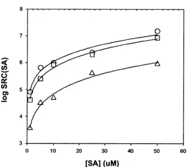
To determine KCuSA and $Cu(SA)2 for each experiment, using Sigmaplot 4.0, we fit values of
SRC(SA) using the equation
log SRC(SA) = log([SA]f 10' K + [SA]f2101*o0) (2.22). The results of this best fit are shown in Fig. 2.3. The best fits gave values and relative errors for logKC.SA and logCu(SA)2 for each salinity. Using these constants, we calculated
new best-fit relationships for the dependency of logKCuSA and logCu(SA)2 on salinity:
logKCSA=(10.90± 0.03) - (0.90± 0.02)log S (2.23a)
and
Values of logKcusA and log Cu(SA)2 obtained for each salinity experiment are shown as circles in Fig. 2.4 (with salinity on a linear scale) along with their best fits (Eqs. 2.23.a and b, heavy black lines). The values reported by Campos (adjusted for pH with Eqs. 2.23a and b) are shown as squares, and their corresponding best fits as light lines. Our values of log Cu(SA)2 agree very well with theirs over the range of salinities, but our results show that logKcusA is significantly higher than what they report.
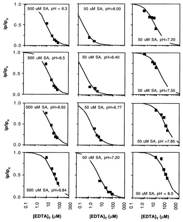
2.3.3. Calibration of SRC(SA) for variation in pH.
We measured values of SRC(SA) at different pH values at salinity = 35%o (Fig. 2.5) to determine whether the relationship between (SRC)SA and pH is best modeled with Eqs. 2.11 a and b (HSA- complexes Cu) or 2.11 c and d (SA2 complexes Cu) (Fig 2.6). In this way we deduce whether HSA- or SA2 complexes Cu, and we can interpolate the
conditional Cu-SA stability constants to any value of pH.
The reported conditional proton dissociation constants at an ionic strength of 1.0 and 0.5 M are pKai = 8.85 and pKa2 = 11.39 and pKai = 8.84 and pKa2 = 11.46, respectively
(Martell, 1993). We used the value for 0.5 M ionic strength because the actual ionic strength of these seawater samples, 0.63 M, is close to 0.5 M, and the values of the conditional proton dissociation constants do not change much from 0.5 to 1.0 M ionic strength. Plugging these values into Eqs. 2.15 and 2.16, we calculated the new ratios of
HSA- or SA2- to [SA]T in the range of pH values from 6 to 9. Then, we substituted these
ratios into Eqs. 2.15 and 2.16 in Eqs. 2.1la-d and divided by the ratios of HSA~ or SA2 to
[SA]f for pH=8.0:
KCuSA,pH= X =KCuSApH=8O ([HSA-] /[SA]f )pH= x (2.24a) ([HSA-] /[SA]f )pH=8.0
and
([HSA-]/[SA],)
pH=x 224)BCu(SA)
2,pH=X = 3 Cu(SA)2,pH=8.0 ([HSA2/[SA]f )2pH=(2b ([HsA-]/[SA],.)
2 pH=8.0 orK~uSA~pH~X K~ O ([SA2-
i]/[SA],)
pH=x (2.24c)CuSA,pH=X
CuSA,pH=8.0 [SA2- ]/[SA],)pH=8.0 and
([SA2-]/[SA],) pH=x
Cu (SA)2 ,pH= X =PCu(SA)
2,pH8.0 ([SA2-] /[SA], )2
pH=8.d
where the value of the conditional stability constant at pH=8.0 is the value we measured for S=35%o at pH=8.0 (Section 2.3.2). Because we are at constant salinity, the activity coefficients remain constant and are included in the conditional stability constants above.
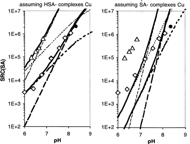
In Fig. 2.6a, the thin dashed and dotted lines for both 50 and 500 pLM SA represent the calculated SRC(SA) for the mono complex and SRC(SA) for the bis complex,
respectively, and the solid lines represent total SRC(SA) calculated using values of KCUSA and Cu(SA)2 adjusted for pH with Eqs. 2.24a and b (assuming HSA- complexes Cu) and either 50 or 200 pM SA. The same is true for the dashed, dotted, and solid lines in Fig. 2.4b, except SRC(SA) was calculated using Eqs. 2.24b and c (assuming SA2 complexes Cu). Clearly the model assuming HSA- complexes Cu best fits the data, and Eqs. 2.8a and b correctly describe the reaction of Cu with SA to make the mono and bis complexes.
In samples with low ionic strength (ie. low salinity samples), the pH calculation will change slightly (see Eqs. 2.13 and 2.14). The pKai for SA at 1%0 is calculated with the Davies Equation to be 8.90, 0.06 log units greater than that reported an ionic strength of
0.5 M. The change in the value of pKa2 will not significantly affect the calculations for
the ratio of [HSA-] to [SA]T at the pH range of interest (6 to 9). Because ionic strength effects change our pH calculations negligibly at different salinities, we used the same values of pKai and pKa2 at 0.5 M ionic strength for all salinities (Chapter 3 and Chapter
5.) However, more precise interpolations could be completed for very low salinities using pKai values calculated for lower salinities.
2.3.4. Ionic strength.
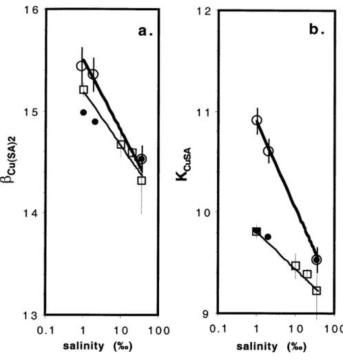
We modeled the changes in logKCuSA and log@Cu(SA)2 as a function of salinity (Fig. 2.4) as
if ionic strength effects (and not competition by Ca2' or another cation with Cu2
, for SA) were the cause for their change. We used the appropriate activity coefficients for Cu24, HSA-, and H' calculated using the Davies Equation. Then, we used activity coefficients
calculated with the Davies Equation to predict the ratio of the values of [HSA-]/[SA]T using Eqs. 2.13 and 2.14. We calculated the new values of KCuSA and Cu(SA)2 expected at
1 and 2%o using Eqs. 2.11a and b. The values calculated are shown in Fig. 2.4 as black
dots. Ionic strength corrections do not fit the salinity dependence of logKCuSA and log0Cu(SA)2 well.
There are at least two possible reasons for the fact that the ionic strength predictions do not fit well the measured data: one theoretical and one analytical. The theoretical reason is that something else besides ionic strength controls SA speciation as a function of salinity; this could include Ca2, or another cation. The NIST database does not offer any
measured values of Ca-SA species, so we are unable to predict whether Ca-SA is important. However, we argue that it is unlikely that Ca2
, or another cation is important at a salinity of 35%o. Because we are able to model the pH effects on SA speciation so
important, then it would be necessary to invoke an SA complex that includes both H' and Ca2
,. . The ionic strength predictions do not fit the Campos (1994) data well either,
suggesting that SA speciation is more complicated than assumed.
2.4.
Conclusions.
We show that Eqs.2.23.a and b can be used to interpolate the approximate values of KCuSA
and $Cu(SA)2 between 1 and 35%o. Values of log@Cu(SA)2 from agree well with those shown previously in Campos (1994), but we found logKCSA to be considerably greater than what they report (Fig. 2.4). Because our extensive data on SRC(SA) at low [SA] are
reproducible and consistent in trend (Fig. 2.2), and Campos and co-workers obtained limited low [SA] low salinity data, we believe that our values are correct.
The values of KCuSA and ICu(SA)2 Can also be independently adjusted for changes in pH
using Eqs. 2.15 (for the case in which HSA~ complexes Cu) at salinity = 35 %o, and, we assume, at lower salinity values.
Predicted ionic strength effects cannot account for the changes in logKCuSA and logCu(SA)2 with salinity. Eqs. 2.23a and b are not appropriate for extrapolating KCuSA andICu(SA)2 for
salinities below 1%o because we have shown that the effect of cation competition (other than SA acid/base speciation) on KCuSA and $Cu(SA)2 may also be important. The
distinction is important for freshwater samples because below 1%o, the value of [Ca2+ and other cations varies widely with stream and watershed chemistry, while the 0.02 M buffer necessary for CLE-ACSV will dominate ionic strength effects. The distinction is also important because our extrapolations of pH dependence at lower salinity assume that H+, and not another cation, dominates SA speciation. Because we see both a pH effect at
salinity = 35%c and a "salinity effect" that is greater than that explicable by ionic strength effects, the speciation of Cu and SA may not be as straightforward as we assume in this chapter. The assumptions of this chapter effect the results and interpretations of field data in Chapters 3 and 5.
References.
(1) Campos, M. L. A. M., C. M. G. van den Berg. 1994 Determination of copper complexation in sea water by cathodic stripping voltammetry and ligand competition with salicylaldoxime. Analytica Chimica Acta. 284, 481-496.
(2) Morel, F. M. M., Hering, J.G. Principles and Applications of Aquatic Chemistry; John Wiley & Sons, Inc.: New York, 1993.
(3) Millero, F. J. M. L. S. Chemical Oceanography; CRC Press, Inc.: Boca Raton,
1991.
(4) Martell, A. E., R. M. Smith, R. J. Motekaitis. Texas A&M University: College Station, 1993.
OH
NOH
CH
Figure 2.2. Ratios of peak height measured in the presence of EDTA to peak height in the absence of EDTA for the calibration of SA dependence on salinity. Raw data (U)
modeled with the average of all values of SRC(SA) obtained from each experiment (black lines). Where more than one line is present, there was more than one experiment conducted (always on different days with different samples). Ratios are also modeled based on the values of SRC(SA) reported by Campos and coworkers (1994) (dashed lines.) Samples with thick frames are combinations of [SA] and salinity for which Campos and coworkers conducted actual experiments.
1* 1 psu, 1 uM SA 0.5 0 - 1.0- 0.5-0.01 1.0-0.5 -0.0 -1.0 0.5- 0.0- 1.0-0.5 -0.0 1 psu, 5 uM SA w4 .. .- .. m-I. . 1 psu, 10 uM SA p . %1 psu, 25 LIM SA e- 0 0 o o 0) C0 1, 0 [EDTA]T (9M) 0 CL - 0C 0 '- I.- o 0 0) C)00 [EDTA]T (jM) 2 psu, 1 uM SA 2 psu, 5 uM SA 2 psu, 10 uM SA 2 psu, 25 uM SA -' 2 psy, 50 uM SA ' -4 0 0 o - C 0 0 '- 0 [EDTAIT (4M) 35 psu, 1 uM SA 35 psu, 5 LIM SA '4. 35 psu,10 uM SA
35 psu, 25 LIM SA'
35 psu, 50 LIM SA , J.4 0 a-0 C-C. 0L 1 s'u,5 I A A iog i
8 L) 0) 3 0 10 20 30 [SA] (uM) 40 50 60
Fig. 2.3. Measured values of SRC(SA) for salinities of (0) 1%o, (0) 2%0, and (A) 35%c, and the best fit of each dataset determined using Sigmaplot 4.0 and Eq. 2.22. The results of the best fits are shown in Eqs. 2.23a, b.
16 12 15 S 11 14 10 13 9 0.1 1 10 100 0.1 1 10 100 salinity (%.) salinity (%.)
Figure 2.4. Values of log $Cu(SA)2 and log KCuSA as a function of salinity measured in this work (0) and from Campos et al (1994) (0). Best fit lines are plotted from Eqs. 23.a and b. The values of log $Cu(SA)2 and log KCuSA at I and 2%0 are predicted using ionic strength arguments from the modeled value of log $Cu(SA)2 (gray dots) and log KCuSA (black dots) at 35%o, using the Davies Equation and the reported value of pKa, for SA (NIST).
a.
b.
1.0 0 C. 0. [EDTAIT (pM) 50 uM SA, pH=6.00 50 uM SA, pH=6.40 ....U ... . ... ... 0.5 500 uM SA, pH = 6.3 500 uM SA, pH=6.5 500 uM SA, pH=6.65 500 uM SA, pH=6.84 C) M A 0 - 'i 0) 0) 0) or [EDTAIT (pM) 50 uM SA, pH=7.20 50 uM SA, pH=7.55 50 uM SA, pH =7.85 50 uM SA, pH = 8.0 T- 0 C0 [EDTA]T (pM)
Figure 2.5. Ratios of peak height measured in the presence of EDTA to peak height in the absence of EDTA for the calibration of SA dependence on salinity. Raw data (U)
modeled with the average of all values of SRC(SA) obtained from each experiment (black lines). 0) 0) 0> T- 0> 0 o= - r 0> 0) 0.0 1.0 0 0.5 0.0 1.0 0 0. 0. 0.5 50 uM SA, pH= 0.0 1.0 0 0. 0. 5 --. . ... .- ... 50 uM SA, pH=7.20 0.5 0.0 .77
assuming HSA- complexes Cu 1 E+7 1E+6 1E+5 1 E+4 1E+3 1E+2 6 a - -/
-/
7 8 1E+7 .i 00 1 E+6 1E+5 1E+4 1E+3 1E+2 9 pH 6 IA
-c~A
I,'j:
I
-I 7 8 pHFigure 2.6. The side reaction coefficient of salicylaldoxime measured at 50 RM SA (0) or
500 pM SA (A). The side reaction coefficent is modeled using the stability constants
determined in Fig. 3 and assuming that either HAS- or SA- complexes Cu (see Eqs. 18.a and 18.b). The SRC(SA) from Campos et al, calculated for 50 pM SA at pH 8.35, is also shown (0). 0 R! W*" F I U p C,) 9
Chapter 3. The contribution of riverine Cu ligands to Cu speciation in
the Saco River estuary
Abstract
Riverine ligands have been proposed to be important to Cu speciation in estuaries and near-shore samples. A few field studies have been attempted to determine whether riverine ligands behave conservatively in a salinity gradient, but these studies did not conclusively show that riverine ligands were important at high salinities and pH values of the estuaries. We analyzed Cu speciation along the salinity gradient at the mouth of the Saco River, ME, to quantify pH and salinity effects on the riverine ligands. We show that riverine ligands, which may be dominated by terrestrial humic substances, can account for all the Cu ligands even
at the sample taken at a salinity of 27%o, even after dilution and changes in binding ability due to pH and salinity effects.
3.1.
Introduction
The toxicity of high concentrations of Cu to plankton (Sunda, 1976; Hall, 1997) and other species is of concern in polluted estuaries and near-shore environments. The toxicity of Cu is related to the concentration of free Cu, [Cu2
1], and not to the concentration of total Cu, [Cu]T. Cu is distributed amongst the "free" form (usually <1% of [Cu]T) and Cu ligands (>99%), so that
[Cu]T=[Cu21]+1[CuLj] (3.1),
where X[CuLi] is the sum of Cu complexed to all the different ligands of type i present in the water column. The extent to which ligands successfully compete with each other for
Cu depends on the relative concentration, [Li], and conditional binding strength KcLi, of each, so that Eq. 3.1 can also be expressed as
[Cu]T=[C 2
U]+KCUL1 [LI]f[CU2 ]+KCuL
2[L 2]f[CU2+]+...+KcuL[Ln][Cu2+] (3.2) where, for this example, ligands of two different sources (and as many as n sources) are present, and [Li]f. is the concentration of the ligand of that source not complexed to Cu, or
[Lj]f=[Lj]T-[CuLi] (3.3)
In order to predict [Cu2
*] and therefore the potential toxic impact of Cu, one needs to
know the concentrations and strengths of all the Cu ligands present in the water column.
There are several possible sources of ligands to an estuary, and from the point of view of the estuary, they can be roughly be divided into the two categories of autochthonous (produced in situ or entrained from bottom sediments) and allochthonous (imported from rivers or terrestrial sources). Autochthonous ligands include microbially produced
ligands (Moffett, 1997; Leal, 1999) and sediment sources of humic substances and sulfide (Skrabal, 2000). Allochthonous sources include microbially produced ligands, terrestrial humic substances (Kogut, 2001; Xue, 1999), sewage effluent and surface runoff (Sedlak,
1997), and riverine dissolved and colloidal sulfides stabilized by complexation with Cu
(Rozan, 1999d). While these two categories share some ligand types (e.g., microbial ligands, reduced sulfide, and humic substances), they serve to distinguish between ligand sources whose importance may depend on estuarine dynamics, such as upwelling,
nutrients loads and Cu concentrations, and those that depend on other factors, such as watershed characteristics, river flowrate, and sewage input (Rozan, 1999d). If we want to be able to predict [Cu2
,] on a long term basis, we must know how the relative inputs of autochthonous and allochthonous ligands change with seasonal or watershed use changes, for example.
Terrestrial humic substances may account for a large fraction of the total Cu speciation in estuaries with large riverine inputs. Humic substances contain a spectrum of Cu binding strengths that can be modeled as organic acids and other ligands with varying strengths e.g., (Bartschat, 1992) or as two or more arbitrary bins of ligands with average
conditional binding constants (Kogut, 2001). Because humic substances have a spectrum of binding sites with varying conditional binding constants, we refer to this spectrum as their "Cu binding ability" over a range of Cu concentrations. The Cu binding ability of terrestrial humic extracts increases with increases in pH and decreases with increased ionic strength effects (Cabaniss, 1988). However, competition with Ca and Mg were not observed to be significant in several studies with SRFA and SRHA (Hering, 1988; Cabaniss, 1988). These studies were conducted at [Cu]T higher than the usual ambient [Cu]T found even in polluted estuaries, but it is likely that the stronger ligands in humic substances are affected by changes in pH and salinity as well. In field samples, an increase in Cu binding upon increase of pH from 8.2 to 9.0 was reported for an estuarine sample (Sunda, 1991). Any study that attempts to quantify the importance of terrestrial humic substances (or riverine ligands in general) to Cu speciation in estuaries and near-shore areas must take into account the effects of salinity and pH on the binding ability of these ligands.
Previous studies to assess the importance of riverine ligands to Cu binding in estuaries show in general that Cu is more strongly bound in low salinity samples than in high salinity samples (van den Berg, 1987; van den Berg, 1986; van den Berg 1990; Apte,
1990; Gardner, 1991). For the first four studies, the pH was held constant at 7.7 - 8.0 in
attempts to maintain the conditional stability constants of these ligands constant and measure the concentrations of ligands along the salinity transect and therefore determine whether riverine ligands behaved conservatively. All four found conservative dilution of
ligands (or in the case of the van den Berg, 1986 study, large variability in ligand concentrations) along the transect. In the fifth study (Gardner, 1991), ligand binding constants and concentrations were obtained at different values of pH and salinity, and it was suggested that the net effect of pH (increasing ligand strength) and salinity effects (decreasing ligand strength) on niverine ligands was null, so that ligand concentrations appeared conservative in the salinity gradient. However, because all these voltammetric studies employed competitive ligand exchange adsorptive cathodic stripping voltammetry
(CLE-ACSV) or ASV calibrated with "internal calibrations", which can significantly
underestimate the importance of humic substances (Moffett, 1997; Kogut, 2001; Voelker, 2001), they likely underestimated the binding ability of riverine ligands. Further, the conditional stability constants of the ligands were allowed to co-vary with ligand concentrations, which may have affected the accurate determination of ligand concentrations (Voelker, 2001). We have successfully developed a new external calibration method that accurately assesses the Cu binding ability of humic substances and of mixtures of stronger and weaker ligands (Kogut, 2001) at different values of pH and salinity (Chapter 2), so that we would be able to avoid all of these problems with previous attempts to determine the importance of riverine ligands in estuaries.
The goal of this study is to increase our understanding of the Cu binding behavior of natural riverine ligands, specifically humic substances, as they travel through an estuary, so that the relative importance of terrestrial and other sources of ligands to estuaries and coastal waters can be assessed more accurately. We analyzed Cu speciation with
CLE-ACSV and our new calibration method in samples taken from a salinity transect in the
Saco River estuary, ME. Iron, which has frequently been shown to flocculate with high molecular weight humic substances, is conservative in this river (Mayer, 1982a),
sediments is negligible. The Saco River is not heavily polluted with Cu and other metals, making it a good site to assess the importance of humic substances in the absence of reduced sulfides, which would likely not be stabilized in high concentrations without high concentrations of metals. The Saco River also has relatively little development near its mouth, so that issues with sewage effluent and anthropogenic chelators are also
minimized.
3.2. Methods
3.2.1. Sample Collection
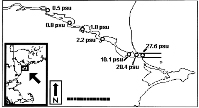
Samples were collected along the salinity gradient in the Saco River in October, 2001, during an incoming tide from a small aluminum boat with an electric outboard motor. Samples for Cu titrations were collected in acid-cleaned Teflon@ bottles just under the surface of the water, from the bow when underway to minimize any contamination from the boat. These samples were "quick frozen" in liquid nitrogen to minimize coagulation of organic matter due to "freezing out" and subsequently stored in a -4*C freezer for three months. Comparison of a riverine sample immediately after sampling and after three months of cold storage shows that this method of sample preservation does not alter the Cu binding ability of the water. Salinity and ambient pH were monitored during sampling using a Hydrolab Minisonde. Salinity was measured again before measurement with a portable conductivity meter (VWR Scientific) calibrated with UV-SW (salinity=35 psu) (Table 3.1.) The pH of each sample was measured again after adjustment with buffer and CLE-ACSV analysis using a pH meter (Orion). Samples to be analyzed for total organic carbon (TOC) and color absorbance were collected in precleaned DOC-free
amber bottles, acidified to pH 3 with phosphoric acid, and stored at +4'C for three months.
3.2.2. Reagents
Buffers were made by adjusting 1.0 M boric acid (EM Science, Suprapur@, pH range of
7.5-8.2), HEPES (OmniPur, pH 7-8), and MOPS (Sigma, pH 6-7)) with concentrated
ammonia (J.T. Baker) or hydrochloric acid (J.T. Baker) until the desired pH was reached.
UV oxidized Sargasso seawater (UV-SW) was collected in August 1997 with trace metal
clean methods and subjected to at least six hours of ultraviolet light oxidation with a medium pressure mercury lamp (Ace Glass, 1000 W). Deionized distilled water (DDW) was from a Millipore Q-H20 system. Fresh 1 mM primary and 1 pM secondary copper
standards were made every day by serial dilutions of an Aldrich atomic absorption standard solution (CuSO4 in 1% HNO3, 10 000 ppm Cu) with DDW; the final pH of the
secondary copper standard was about 6. Salicylaldoxime (Aldrich) was purified by repeated filtering and recrystallization from solutions containing 1 mM EDTA (Campos,
1994). SA was dissolved in DDW for a final stock solution concentration of 0.025 M.
SA stock solutions were replaced monthly and refrigerated when not in use.
Acid-cleaned Teflon@ or polycarbonate containers were used for all reagents and experiments to minimize adsorption of copper and ligands to bottle surfaces and leaching of phthalate plasticizers into the samples.
3.2.3. Filtering
Cu speciation samples were syringe-filtered through acid cleaned 0.2 pm polycarbonate membrane filters (Nucleopore, 47 mm filter diameter) sandwiched in acid-cleaned
polycarbonate filter holders. This filtration protocol does not add significant concentrations of Cu or strong Cu ligands (Chapter 4).
3.2.4. Total organic carbon and color
Samples for total organic carbon (TOC) measurements were acidified to pH=3 with phosphoric acid (J.T. Baker) and TOC was measured using a Shimadzu TOC-5000 analyzer calibrated with diluted solutions of a 1mg/ml potassium acid phthalate standard (VWR Scientific). Absorbance of the sample at 350 nm (with the absorbance at 500 nm subtracted) was measured with Hewlett-Packard 8543 UV-visible photospectrometer.
3.2.5. Total Cu.
Samples from each filter fraction were acidified to pH < 2 with concentrated nitric acid
(J.T. Baker Instra-Analyzed) and irradiated with ultraviolet light from a mercury lamp
(Ace Glass, 1000 W) for at least six hours in quartz 125 ml tubes. Samples were then brought to circumneutral pH and analyzed with CLE-ACSV. With all ligands destroyed,
[Cu]T,O in the original sample is [Cu(SA)x] in the sample, which is measured as described below.
3.2.6. CLE-ACSV
CLE-ACSV is a two-part process: first, a known concentration of a well-characterized
and purified synthetic ligand is allowed to equilibrate with a series of samples containing a range of concentrations of added copper. Salicylaldoxime (SA) is a very strong, well-characterized added ligand which partitions only negligibly into natural organic matter at concentrations typical of rivers and coastal areas (Appendix B). In the presence of SA,
Cu species include free Cu, Cu complexed by ligands in the sample, and Cu complexed
by SA:
[Cu]T = [Cu2
1] + I[CuLi] + X[Cu(SA),] (3.4)
where
X[Cu(SA),] = [Cu(SA)] + [Cu(SA)2] (3.5)
and Cu(SA) and Cu(SA)2 are the mono and the bis complexes of copper with SA,
respectively (both complexes are important at the concentrations of SA used).
The value of X[Cu(SA).] in the samples is analyzed using adsorptive cathodic stripping voltammetry, ACSV, which is discussed in more detail in Appendix D. For ACSV, Cu-SA complexes adsorb to the surface of the mercury drop electrode and Cu2> in the Cu-SA complexes on the drop is reduced during a negative potential scan, which produces a peak current with magnitude ip. The relationship between the current peak height, i, and X[Cu(SA)], called the sensitivity, S:
I[Cu(SA)x] = ip/S (3.6),
must be determined in the absence of ligands that compete with SA for Cu, so that any additional Cu added (A[Cu]T) is complexed only by SA:
A[Cu]T ~ AZ[Cu(SA)x] (3.7).
S depends on both instrument settings (e.g. adsorption time and potential) and the sample matrix. The "internal calibration", a method commonly used to determine the sensitivity, assumes that for each titration, ligands in the sample are "titrated out" at higher [CulT and therefore Eq. 3.7 applies to this region of the titration. We found that this assumption is false for samples which contain humic substances or other mixtures of heterogeneous ligands, and we developed a more robust technique we call an "overload" titration (Kogut, 2001). For the overload titration method, at least two Cu titrations (with
concentrations outcompetes all of the natural ligands present in the sample, so that Eq.
3.7 applies to this titration. The sensitivity of one overload titration is then used to
determine titrations at lower [SA] ("speciation titrations") which are designed to allow the ligands in the sample to compete effectively with SA and therefore reveal information about the binding ability of those ligands.
We need correction factors to extrapolate S from overload titrations with high [SA] to speciation titrations with low [SA] because S depends somewhat on SA (see Appendix
C). The correction factors are obtained by comparing S at high and low [SA] in
sub-samples that have been UV-irradiated to destroy all ligands that could compete
successfully with low [SA]. The correction factors depend in part on instrument settings as well as sample salinity and pH, may be related to changes in Cu-SA speciation on the surface of the mercury drop during CSV analysis (Campos, 1994; Appendix D), and range in value from 0.3 to 1.0 in the samples we have analyzed. We successfully used correction factors with overload titrations to relate peak heights to X[Cu(SA)x] in humic extract solutions (Appendix D).
3.2.7. Setup for Cu overload and speciation titrations.
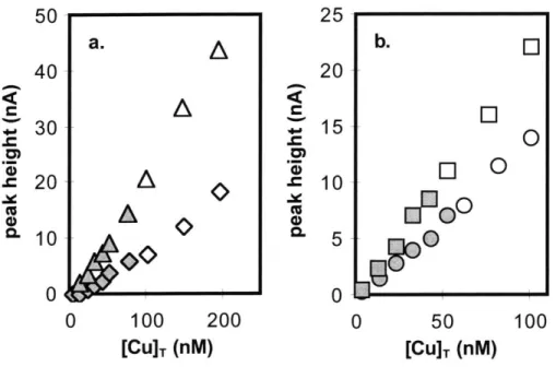
For overload and speciation Cu titrations, 10.0 ml of the sample was pipeted directly into the electrode's Teflon@ sample cup. A buffer adjusted to the pH desired was added for a final concentration of 0.02 M. SA (1, 3, 5, or 10 pM for speciation titrations and 100 pM for overload titrations and [Cu]T,O analysis) was also added to the sample at this time. Copper from the secondary standard was added sequentially after each titration point for a range of added [Cu]T from 10 to 200 nM. Before each voltammetric analysis, samples were allowed to equilibrate for 3 minutes. Overlapping overload titrations at 25 and 50
pM SA for the 0.5% Saco River sample show that 25 pM SA outcompetes all natural ligands for Cu (data not shown.) Overlapping titrations with different SA show that 3 minutes is adequate time for equilibration amongst Cu, SA, and the ligands present (see Results).
3.2.8. Cu speciation titrations.
We conduct multiple Cu titrations of each sample to collect data on a range of Cu ligands from those that control Cu speciation at a relevant range of [Cu]T. For each titration point, in the absence of both SA and the Cu complexed by SA, the water sample would have an identical [Cu2
1] and a theoretical total copper concentration [Cu]T* that is given
by:
[Cu]T* = [Cu] - I[Cu(SA)x] = [Cu2+] + I[CuLj] ~ X[CuL] (3.8),
where [Cu2
+] is negligible compared to I[CuLi]. The value of [Cu21] is calculated from I[Cu(SA)x], [SAlT, and the conditional stability constants of the mono and bis complexes,
KCu(SA) andICu(SA)2
[Cu2 ]=X[Cu(SA)]/(KC(SA)[SA]f+$Cu(SA)2[SA]f2) (3.9)
where [SA]f is the concentration of SA not bound to copper:
[SA] = [SA]T - [Cu(SA)] - 2[Cu(SA)2] (3.10),
calculated using EXCEL to solve for the four unknowns in the four equations (Eqs. 3.9 and 10 and the two equilibrium mass law expressions for formation of Cu-SA
complexes.) The presentation of Cu speciation data in plots of [Cu2
+] versus [Cu]T* shows the binding ability of the sample in the range of [Cu]T* for which data was collected. Where more or stronger ligands are present in the sample, [Cu2
1] is lower at any single value of [Cu]T*. The data can be modeled with FITEQL or another modeling program as concentrations of one or more ligands each with an average KcLi, but these
types of fits might not provide meaningful constants and should be used carefully (Voelker, 2001).
3.3. Results
3.3.1. Cu speciation in Saco River estuary
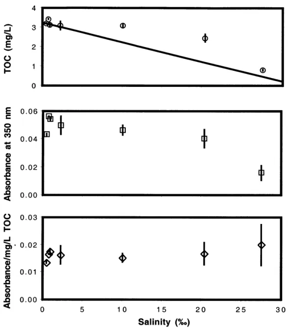
We hypothesize that riverine ligands in general are a major source of ligands to estuaries and coastal areas, even after dilution and potential decrease of their binding ability by cation competition and ionic strength effects. Because we further hypothesize that terrestrial humic substances can dominate Cu speciation in rivers and estuaries, we measured TOC and light absorption at 350 nm as potential tracers of humic substances in each sample of the Saco River estuary (Fig. 3.2). Non-conservative behavior indicates a
source or sink of TOC in estuary, or that the system is not at steady state (Fig 3.1). .Absorbance of the samples at 350 nm shows similar behavior to that of the TOC and appears to be roughly proportional to TOC.
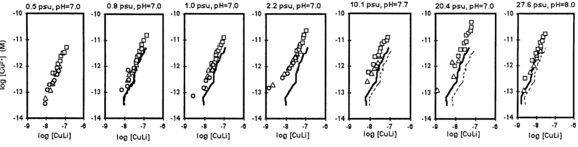
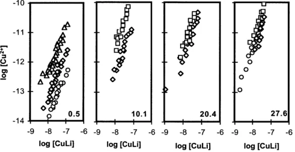
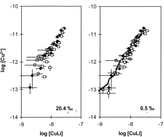
We determined the Cu binding ability of each sample using our new SA constants corrected for pH and salinity. Fig. 3.3(a-g) shows [Cu2
,] as a function of [Cu]T* in each sample, along with the corresponding salinity and pH (after the addition of buffer) for that sample. The pH at which Cu speciation was determined (controlled with added buffer) is usually within 0.2 pH units of the original pH of the sample. Heavy black lines in Fig. 3.3(b-g) represent the Cu binding ability of the ligands in the riverine end member (salinity = 0.5%o) (Fig. 3.3a) as if only dilution with seawater were important for