Economic Policy October 2004 Printed in Great Britain © CEPR, CES, MSH, 2004.
The pillar
s of
the ECB
Blackwell Publishing, Ltd.Economic PolicyOxford, UK0266-4658ECOP © Blackwell Publishing 2004Original Article40 THE PILLARS OF THE ECBSTEFAN GERLACH
SUMMARY
I interpret the European Central Bank’s two-pillar strategy by proposing an empirical model for inflation that distinguishes between the short- and long-run components of inflation. The latter component depends on an exponentially weighted moving average of past monetary growth and the former on the output gap. Estimates for the 1971–2003 period suggest that money can be combined with other indicators to form the ‘broadly based assessment of the outlook for future price developments’ that constitutes the ECB’s second pillar. However, the analysis does not suggest that money should be treated differently from other indicators. While money is a useful policy indicator, all relevant indicators should be assessed in an integrated manner, and a separate pillar focused on monetary aggregates does not appear necessary.
Economic Policy October 2004 pp. 389– 439 Printed in Great Britain © CEPR, CES, MSH, 2004.
The Pillars of The ECB
The two pillars of the European
Central Bank
Stefan Gerlach
Hong Kong Institute for Monetary Research, University of Basel, and CEPR
1. INTRODUCTION
‘Pillar. 1. A detached vertical structure of . . . solid material, . . . used either as a vertical support of some superstructure, as a stable point of attachment of some-thing heavy and oscillatory, or standing alone as a conspicuous monument or ornament; . . .’ (The Compact Edition of the Oxford English Dictionary, Vol. II, 1984, p. 2175).
As the above quotation illustrates, the term ‘pillar’ has several meanings ( in fact, the OED gives another eleven definitions of ‘pillar’). It is perhaps therefore not surprising that after more than five years of operation, the monetary policy strategy of the European Central Bank (ECB) remains highly controversial. Initially announced in October
I am grateful to the editors and discussants, to other Panel meeting participants, and two referees. I also thank seminar participants at the ECB and De Nederlandsche Bank; Huw Pill and Cees Ullersma, my discussants at those seminars; Michael Chui and Petra Gerlach-Kristen for comments; and Maritta Pavloviita for data. I would also like to record my gratitude to Claus Brand, Alistair Dieppe, Gabriel Fagan, Dieter Gerdesmeier, Hans-Joachim Klöckers, Jérôme Henry, Ricardo Mestre and Barbara Roffia at the ECB for giving me access to data which I have used for several papers, including this. The views expressed are solely my own and not necessarily those of the institutions that I am affiliated with.
1998, the hallmark of the strategy is the use of ‘two pillars’ in formulating and setting monetary policy.1 The first pillar, which is defined as a:
‘prominent role for money, as signalled by the announcement of a reference value for the growth of a broad monetary aggregate’,
has remained the object of a lively debate and has been subject to intense criticism.2
For instance, Begg et al. (2002, p. xiv), writing in the CEPR Monitoring the European
Central Bank series, state that:
‘the first pillar of the monetary strategy is now flawed beyond repair – both as a matter of theory and empirically’.
By contrast, the second pillar, defined by the ECB as a:
‘broadly based assessment of the outlook for future price developments and the risks to price stability in the euro area as a whole’,
has been accepted by the public and the economics profession as a natural part of any active monetary policy strategy. Of course, all central banks that gear monetary policy to achieving and maintaining price stability presumably rely on such an assess-ment in setting interest rates. So why has the monetary pillar become so exceedingly controversial?
1.1. The issues
One reason for the controversy as regards the ECB’s monetary pillar is that observers have failed to detect any relationship between the growth rate of M3 and interest rate decisions taken by the Governing Council of the Eurosystem. With the exception of Gerdesmeier and Roffia (2003), econometric estimates of reaction functions for the euro area typically fail to find that money growth plays a role in the ECB’s interest rate decisions. Furthermore, in commenting on the reasons for its policy decisions, the Governing Council has repeatedly stated that episodes of rapid money growth were due to special factors and/or shifts in the demand for money arising from changes in portfolio preferences or in the opportunity cost of holding money. For this reason, it interpreted the observed money growth as not signalling ‘risks to price
stability’ and therefore chose to disregard it. Galí et al. (2004) review the statements
1
The ECB’s policy framework is reviewed in ‘The stability-oriented monetary policy strategy of the Eurosystem’, ECB Monthly Bulletin, January 1999, pp. 39 – 50. For a non-technical review, see ECB (2004). The role of money in the strategy is discussed in ‘Euro area monetary aggregates and their role in the Eurosystem’s monetary policy strategy’, ECB Monthly Bulletin, February 1999, pp. 29 – 46. Svensson (1999) contains an early but still highly relevant critique of the ECB’s monetary policy strategy. See also Svensson (2002).
2 Reviewing the critique of the two-pillar framework goes beyond the scope of this study. In Box 1, I instead summarize the
analysis in the last report in the CEPR series on Monitoring the ECB 5 (Galí et al. 2004), which provides a critical review of a number of arguments in support of the first pillar.
about economic conditions in the Editorials in the ECB’s Monthly Bulletin and conclude that the Governing Council typically interpreted money growth as not worrying even when it exceeded the 4.5% reference value (see also Gerlach, 2004). Strikingly, despite the fact that money growth was above the reference value between July 2001 and September 2003, the Governing Council never took the view that rapid money growth warranted a tightening of monetary policy.3
An arguably more important reason for the controversy surrounding the frame-work is that the ECB has not spelled out in detail its view of the exact role of money in the inflation process and in the setting of interest rates. Indeed, the ECB has never provided a formal explanation for why it believes that money growth and prices are linked over time and, in particular, why it interprets this relationship as reflecting causation, rather than merely correlation. Indeed, as noted by Galí (2003), a direct relationship between money growth and inflation arises from the existence of a stable money demand function irrespectively of the monetary policy strategy followed by the central bank. Furthermore, in discussing the role of money in its strategy and conduct of policy the ECB has tended to use imprecise terminology. For instance, it has emphasized the ‘medium-term’ orientation of the framework and has repeatedly used the notion of a ‘monetary overhang’ but has never given these concepts unam-biguous definitions. It has also asserted that money growth has been disturbed by ‘special factors’ without necessarily being too clear about whether they were of a once-off nature or could be expected to return. Many observers have arguably inter-preted this, rightly or wrongly, as the ECB having given the monetary pillar an extra degree of freedom by its choice of terminology.
For the ECB to overcome the scepticism that surrounds the monetary pillar, it needs to provide a clearer explanation of the role of money in the inflation process than it has to date. This necessarily requires a formal, estimable model of the inflation process and the role of money in it. The existence of such a model would naturally shift the debate from the general level that characterizes the exchange between the ECB and its critics today, to the concrete level at which economics is typically debated in the literature. Instead of arguing about whether the framework is ‘sensible’, the debate would move to technical questions such as whether the model could be derived from first principles, how it should be estimated, whether the resulting estimates are stable over time, whether the empirical results provide support for the two-pillar model, and so on. It is precisely for this reason that central banks, in particular those with inflation targets, tend to make public the models they use to forecast inflation. Formalization is helpful in that it makes
3 In presenting the framework, however, the ECB did emphasize that it would not change interest rates automatically in response
to changes in money growth: ‘the concept of a reference value does not entail a commitment on the part of the Eurosystem to correct deviations of monetary growth from the reference value of the short term. Interest rates will not be changed “mecha-nistically” in response to such deviations in an attempt to return monetary growth to the reference value.’ (ECB Monthly Bulletin, January 1999, p. 49).
it possible to pin down the exact nature of the disagreement(s) and the areas of agreement.
In light of this, one would have expected the ECB to put forth a formal model of its framework. Rather than doing so, however, when discussing its two-pillar strategy ( ECB Monthly Bulletin, November 2000, pp. 37 – 48) it has stated that:
‘it has proven extremely difficult to integrate an active role for money in conven-tional real economy models . . . despite the general consensus that inflation is ultimately a monetary phenomenon’ ( p. 45).
In discussing the two pillars, it has gone on to assert that:
‘it is not practically feasible to combine these two forms of analysis in a transparent manner in a single analytical approach’ ( p. 46).
While seemingly innocuous, these statements are thought provoking. Why, one may wonder, did the ECB adopt a monetary policy framework that it has found difficult to rationalize using standard macroeconomic analysis? Isn’t the mere fact that it is difficult to formalize the two pillars in a clear and transparent fashion a good reason to worry about, or even doubt, the usefulness of such a policy framework?
Given the need for a model of the ECB’s two-pillar framework, seeking to formalize it should be high on the research agenda. This paper provides an attempt to do so by proposing a simple ad hoc empirical model of inflation in the euro area.4 The
model, which incorporates money growth in a Phillips curve, interprets the two pillars as separate approaches to forecasting inflation at different time horizons. The first pillar – the monetary analysis – is seen as a way to forecast inflation at long time horizons and to account for changes in the steady-state rate of inflation (or in the average rate of inflation over a few years). Empirically, I associate the first pillar with an exponentially declining moving average of M3 growth.5 The second pillar – the economic analysis – is understood as the ECB’s way to predict short-run movements in
inflation around that steady-state level. The model identifies the output gap with the second pillar; a more elaborate version would need to consider also other determi-nants of temporary swings in inflation, including import and energy prices, changes in value added taxes and so on.
4
There are several other studies on the role of money in the euro area, but, with the exception of Neumann (2003), these do not focus on interpreting the two-pillar framework as I do here. Andrés et al. (2003), following Ireland (2002), study the role of money by estimating a small-scale dynamic general equilibrium model in which real balances may affect the marginal utility of consumption, but find no evidence for such an effect. Coenen et al. (2001) estimate a model in which money contains informa-tion about output, which is measured with error. Andrés et al. (2004), Kajanoja (2003) and Lippi and Neri (2003) estimate forward-looking money-demand models that imply that money may contain useful information about the state of economy that is not embedded in currently observed variables.
1.2. Outline and main results
The paper makes two contributions. The first of these is to demonstrate, as others have done before, that money growth does contain information about future inflation in the euro area and that money therefore can serve as an information variable. I argue, however, that the analysis does not support the notion that money should be treated any differently from other information variables and, in this sense, does not point to a need for a separate monetary pillar. Indeed, the second contribution of the paper is to show how money growth can be integrated with other information variables to forecast inflation and to form the ‘broadly based assessment of the outlook for future price developments and the risks to price stability’ that constitutes the second pillar of the ECB’s framework.
Section 2 characterizes briefly the joint behaviour of inflation and money growth in the euro area. I show that these variables are closely correlated. Section 3 presents some evidence to the effect that (a measure of ) money growth contained information for future inflation in the 1970 –2003 period, even after accounting for the informa-tion in past inflainforma-tion and the output gap. Estimates for subperiods show that while money was informative for future inflation in the 1970 – 86 period, the information content declined after 1987. Section 4 argues that the two-pillar framework must ultimately rely on a two-pillar view of inflation. It goes on to propose an empirical model of inflation – a ‘two-pillar Phillips curve’ – that integrates money with a standard, although forward-looking, Phillips curve and provides a composite forecasting model for inflation. Section 5 proceeds to estimate the model using data for the 1971–2003 period. Without going through the results in detail here, I argue that the model fits the data well. Section 6 provides estimates for two subsamples. The first of these spans the high inflation period 1971–91, and the second the low inflation period 1992–2003. Perhaps surprisingly, I find that the model fits well also in the latter sample period. Four boxes and two appendixes complement the analysis in the main part of the paper. Box 1 summarizes the analysis in the last report in the CEPR series on
Monitoring the ECB (Galí et al., 2004), which provides a critical review of a number of
arguments in support of the first pillar. Box 2 surveys research published by the ECB on the information content of money growth for inflation. Box 3 reviews how the role of money growth in the ECB’s policy strategy was changed as a consequence of the review of the framework that was completed in May 2003. Box 4 provides a formal statement of the empirical model and the resulting inflation equation that I estimate. Appendix 1 provides some new results on the usefulness of money in forecast-ing inflation in the euro area and Appendix 2 derives the inflation equation that I estimate.
In Section 7 I conclude by turning to the central question whether the model and the broader literature on money growth and inflation provide support for a monetary pillar. I claim that money growth is about as useful for predicting future inflation in the euro area as the output gap, and that it consequently makes good sense for the
ECB to monitor monetary developments in the same way as it assesses other indica-tors of price pressures. Next I turn to the question of the monetary pillar. I argue that while money is a useful policy indicator, all such indicators should be assessed in an integrated manner. Thus, I do not believe that the analysis implies that a separate monetary pillar is necessary.
Box 1. Monitoring the ECB 5
Reviewing in detail the large literature criticizing the two-pillar strategy would go far beyond the scope of the present paper. This box instead summarizes the analysis of a number of claims in favour of a monetary pillar in the most recent of the annual reports by the CEPR on ‘Monitoring the ECB’, entitled, The
Monetary Policy Strategy of the ECB Reconsidered (Galí et al., 2004; needless to say,
my interpretation of these arguments may or may not coincide with those of my co-authors).
One argument in support of the first pillar is that money may be a proxy for
variables that are observed with a lag or not at all. For instance, output gaps, which play
an important role in most central banks’ analysis of inflation, are unobserved and measures thereof must be constructed using data that are published with a lag and may undergo repeated revisions. Since money growth data are rapidly available and money may be correlated with income, it could potentially be used to improve assessments of the current output gap. However, the report argues that other, non-monetary variables are likely to be more informative than money for this purpose. Furthermore, even if money did contain useful information, there is no reason to give it a separate pillar. Rather, the infor-mation in money should be used together with other indicators in forming a broader view of economic conditions.
A further alleged reason for why it may be helpful to monitor money growth is that money may play an important role in the transmission mechanism of
monetary policy. The report analyses this argument but concludes that while
it may well be correct, it would suggest looking at more direct measures of the financial conditions of firms and households than the growth rate of the broad money stock. Moreover, also in this case would it be natural to undertake this work as a part of the economic analysis underlying the second pillar.
Another claim for why money growth needs to be monitored is that high inflation is always associated with rapid money growth, which in turn suggests that monetary control is essential for ensuring long-run price stability. While the report does not dispute that growth rates of money and prices are frequently closely related (in the sense that money and prices may be cointegrated), it argues that
this is not sufficient to justify a monetary pillar. A finding of cointegration does not imply that prices adjust to money. In a multivariate setting in which money and prices are cointegrated with, say, income and interest rates, the adjustment to equilibrium may be carried out by movements in the latter variables rather than money or prices. Thus, money being high relative to prices might well lead to lower money growth in the future. Moreover, to the extent that prices adjust, they need not do so rapidly. Overall, cointegration between money and prices does not impose much restriction, if any, on the short-run behaviour of inflation. Optimizing inflation control therefore requires policy-makers to focus on other, short-run factors that are presumably captured in the economic analysis of the second pillar.
It is sometimes asserted that while the economic analysis of the second pillar
may serve to ensure price stability in the short term, this is not sufficient to safeguard price stability in the long run. Here the report takes the view that
maintain-ing price stability month-by-month presumably must imply maintainmaintain-ing it over the long run as well. Moreover, while the report is open to the notion that there could indeed be potential medium-term risks to price stabil-ity, it argues that the ECB’s strategy does not at all spell out what policy reactions these should elicit as long as that threat remains merely potential. The usefulness of indicators of medium to long-term risks to price stability is therefore unclear.
It has been argued that conducting monetary policy with an eye on money growth may
be useful for avoiding the trap of discretionary policy-making with a resultant increase in inflation. While avoiding an inflation bias due to discretionary policy is desirable,
the report concludes that this problem is better solved by the ECB committing itself to following an appropriately designed policy rule rather than adopting a two-pillar strategy.
Yet another argument in favour of monitoring money is that the two-pillar
strategy leads to more robust decision-making by cross-checking the implications for interest rates of alternative models of inflation. While the report recognizes the
need for such cross-checking, this could presumably be done in the context of the economic analysis in the second pillar, which should take into account all information regarding inflation pressures including information about the role of money growth in the inflation process. The report also notes that the ECB has never spelled out in detail what the role of money is in the alternative models of the inflation process it has in mind, and that the ECB appears to view monetary analysis as providing an escape clause for policy. Thus, the ECB seems to argue that although that analysis does not lead to formal inflation forecasts, it helps guard against inflation gradually rising above the objective. The report is recognizant of the need to guard against this and notes that limiting money growth may be one way in which persistently high inflation can be avoided. However, it goes on to argue that a more
natural and better way to achieve this is simply to monitor actual inflation developments.
The final argument considered by the report is the claim that monitoring
monetary aggregates is essential to preventing instability due to self-fulfilling expectations.
The report analyzes this argument, but concludes that many of these problems can be overcome with interest rate rules (see the discussion in Woodford, 2003). The potential exception is the case of self-fulfilling deflation-ary traps in case of which the report argues that a commitment by the central bank to maintain money balances at a level above that required to keep the interest rate at zero may be desirable (as discussed by Eggertsen and Woodford, 2003). However, this is only necessary in specific circumstances, and does not generally involve cross-checking in the form of a two-pillar policy framework.
My own interpretation of the report is that it takes the view that the ECB would be ill advised to disregard monetary factors, but that taking proper account of these does neither necessarily entail monitoring the growth rate of M3, nor does it require a separate monetary pillar.
2. MONEY GROWTH AND INFLATION: EMPIRICAL REGULARITIES
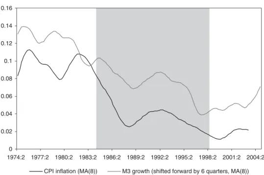
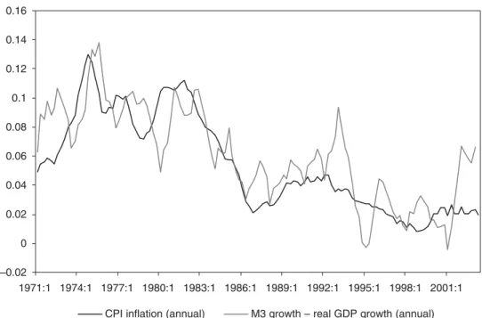
To motivate the subsequent analysis, it is useful to start by looking at the behaviour of inflation and money in the euro area. Figure 1 shows the evolution of CPI inflation and money growth since 1971.6 Following the practice of the ECB and most other
central banks, both growth rates are computed as the change over four quarters. The figure tells a familiar story: money growth and inflation were both high in the 1970, declined and reached a low around 1986, and then accelerated until 1991. Subse-quently both decelerated before increasing somewhat towards the end of the sample. The ECB views these correlations as reflecting the impact of money growth on future inflation. In the Monthly Bulletin of February 1999 ( p. 39), it provides a figure of an eight-quarter moving average of four-quarter inflation and money growth, with money growth led six quarters, presumably because this captures the lag between movements in money and prices. Figure 2 provides an updated version of this plot, with the data starting in 1972Q4 and ending in 2003Q1. To facilitate a comparison, the sample period used in the figure in the Monthly Bulletin is also indicated.
The figure shows a close relationship between the two series. However, that relationship was somewhat less close in the 1972 – 83 and the 1999 – 2003 periods that were not included in the figure in the Monthly Bulletin.
6
Prices are measured by consumer prices, money by M3 and output by real GDP. All variables are seasonally adjusted. The data set and information about its construction are available at http://www.economic-policy.org.
Figure 1. CPI inflation and M3 growth
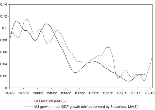
Figure 2. CPI inflation and M3 growth (6 quarters earlier)
Of course, the quantity theory suggests that the relationship between money growth and inflation depends on output growth and on velocity. While the ECB has taken the view that velocity is declining at a broadly stable rate over time (see Brand et al., 2002), income growth does fluctuate. Figure 3 therefore contains a plot of inflation together with the growth rate of M3 minus the growth rate of real GDP ( in what follows, I refer to this as money growth adjusted for income growth or ‘adjusted money growth’).7 The relationship between inflation and adjusted money growth
is perhaps even closer than the relationship between inflation and money growth. However, Figure 4, which is constructed in the same way as Figure 2, does not show any lag between adjusted money growth and inflation. This casts some doubt on the empirical regularity emphasized by the ECB in motivating the mone-tary pillar.
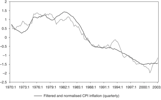
Further evidence on the relationship between money growth and prices in the euro area is provided by Gerlach (2003) who, following Cogley (2002), studies the behav-iour of exponentially weighted moving averages of inflation and adjusted M3 growth obtained using a simple filter.8 Here I simply note that applying the filter to an
economic series, or ‘filtering’ the series, produces a more slowly moving series that I
7
Alternatively, it could be thought of as the growth of money per unit output.
8 In a paper related to Gerlach (2003), Neumann (2003) employs the Hodrick–Prescott filter to obtain a two-sided moving
average of money growth and uses the resulting time series to model inflation in the euro area. Jaeger (2003) uses spectral analysis to study the relationship between money growth and inflation in the euro area in the short and long run.
refer to as the ‘trend’ version of the series in question. Thus, applying the filter to money growth, adjusted money growth or inflation generates ‘trend money growth’, ‘adjusted trend money growth’ and ‘trend inflation’. The extent of the filtering depends on a ‘smoothing parameter’ which determines how smoothly the filtered series evolves over time. I assume the 0.075 value used by Gerlach (2003), which implies a half-life of 9.2 quarters; in the econometric analysis below I estimate this parameter (see Box 4 below for technical details).
Because of velocity shocks, there is no reason to expect a one-to-one relationship between trend inflation and money growth. To see more clearly the correlations between the variables, I therefore transform the data so that they have zero mean and unit variance. Figure 5 plots filtered inflation and M3 growth and Figure 6 plots filtered inflation and adjusted M3 growth. The figures show a close relation-ship between trend inflation and money growth, in particular adjusted money growth.9
Overall, these informal time series plots are supportive of a tight link between money and inflation in the euro area and are no doubt one reason why the ECB believes that a two-pillar framework is appropriate. As noted above, however, a relationship between money growth and inflation arises from the existence of a
9 Lucas (1980) discusses how filtering can be used to clarify the relationship between inflation and money growth.
Figure 5. Filtered and normalized CPI inflation and M3 growth
money demand relationship. Thus, these figures are silent on the critical issue whether it is money growth that leads to inflation or inflation that leads to money growth.
3. MONEY AND PRICES: REDUCED-FORM EVIDENCE
Next I characterize the relationship between money growth and inflation somewhat more formally. While the figures reviewed above suggest that different measures of money growth are correlated with future inflation and therefore may contain infor-mation useful in judging ‘risks to price stability’, they by no means provide any firm evidence to that effect. For money to be a useful information variable, it must be that it contains information that is not already embedded in past inflation rates or other traditional indicator variables, in particular measures of the output gap. A large body of research conducted by the ECB and others demonstrates that money growth does contain such information (see Box 2). As a prelude to the econometric analysis, I explore the information content for future changes in inflation of the trend money growth measure discussed above.
Box 2. Money and inflation in the euro area
Much of the research on the relationship between money and prices in the euro area has focused on modelling the demand for money and has been contributed by the staff of the ECB. Masuch et al. (2003) summarize work in this area by the ECB; its predecessor, the European Monetary Institute, also conducted research on this issue: see, e.g., Fagan and Henry (1998). Coenen and Vega (2001) study quarterly data on real M3, real income, short and long interest rates and inflation for the period 1980 – 98. After testing for weak exogeneity, they estimate a single equation error-correction model, which appears stable and well behaved, for the demand for the real money stock. Brand and Cassola (2000) study the same variables over a slightly longer sample, and estimate a system comprising three long-run relationships. They also find a well-defined money demand relationship and detect no evidence of instability.
Calza et al. (2001) investigate the demand for money in the euro area. In contrast to the earlier literature, the authors focus on measuring the opportu-nity cost of holding M3 and argue that it is best captured by the spread between short-term interest rates and the own return on M3. They also esti-mate a system consisting of a demand equation for the real money stock and an equation for the opportunity cost. This system appears to have good statis-tical properties and to be stable. Fagan et al. (2001) estimate a money demand
function as one equation of their econometric model of the euro area in which, as noted by Begg et al. (2002), money plays a purely passive role. Brand et al. (2002) study the income velocity of money in the euro area, which is of import-ance in the determination of the ECB’s reference value for M3 growth. They find a well-defined empirical relationship between money, income, prices and the opportunity cost of holding money. However, there is some limited evidence that the income elasticity of money demand has risen from 1992Q1 onwards.
The models studied above all focus on the demand for the real money stock, and find that it moves over time to offset monetary disequilibria as captured by an error-correction term. One unfortunate implication of the use of the real money stock in the analysis is that the results are silent on whether it is the nominal money stock or the price level (or both) that adjust to offset disequi-libria. Thus, these models do not permit conclusions to be drawn regarding the role of money in the inflation process.
The relationship between money and prices has been addressed directly by Trecroci and Vega (2000). They argue that while money does not appear to Granger cause inflation, that conclusion depends on the information set used in the forecasting exercise. Moreover, they find that the ‘p-star’ model – or, equivalently, the real money gap model of Gerlach and Svensson (2003) – indicates that money is informative about future inflation. Although the authors argue that the model can be refined, they show that it provides better longer-term forecasts of inflation than the non-monetary inflation equation in the econometric model of Fagan et al. (2001). Nicoletti-Altamari (2001) per-forms a simulated out-of-sample forecasting exercise to study the information content of money for prices in the euro area. The results suggest that monetary and credit aggregates provide useful information about price developments, particularly at medium-term horizons.
Batini (2002), in an ECB working paper, studies the relationship between money and prices in the euro area in a model-free manner. She finds that money growth, which she interprets as a measure of overall monetary condi-tions, impacts on inflation with a time lag of over a year.
While the findings discussed above are all compatible with the notion that money contains information that is useful in predicting inflation, it should be remembered that the results stem from non-structural models. They are therefore arguably best seen as establishing the empirical regularities that are to be explained.
Overall, I interpret this literature as indicating that money has predictive content for inflation in the euro area. However, the output gap is also relevant for forecasting inflation.
My approach is similar to that of Cogley (2002), who uses (what I call) trend inflation as a measure of core inflation and asks whether the discrepancy between headline and trend inflation is useful for predicting future changes in headline inflation. More formally, Cogley explores whether the change in headline inflation over the coming j quarters is predictable on the basis of the current spread between trend and headline inflation. He also generalizes this approach by asking how these results change if other variables are included in the analysis. As additional variables I incor-porate the output gap and the spread between current trend money growth and trend inflation. My principal interest is to explore whether this latter variable is statistically significant and how it contributes to the explanatory power of the regression.
Before turning to the results three comments are in order. First, I focus on the wedge between trend money growth and trend inflation since it plays an important role in the analysis below and since its information content has not previously been studied. Of course, other measures of money, in particular ‘headline’ money growth, could also be used. Second, this is a reduced-form relationship. Woodford (1994) demonstrates that the usefulness of an information variable (in my case money growth) for forecasting a target variable (in my case inflation) depends on the policy regime in force. Woodford’s argument implies that the correlation between money growth and inflation can be zero even if money is a structural determinant of infla-tion. Thus, a finding that money growth does not contain information about future inflation does not necessarily imply that money growth is irrelevant, from a structural perspective, for price formation. Moreover, the information content of money may shift over time in response to changes in the policy regime. Third, econometric work on the usefulness of information variables is inherently subject to the critique that the results are only valid in the estimation period. Since I am interested in whether a proposed information variable is operational at monetary-policy relevant time horizons, say 1–3 years ahead, one needs at least a sample several times longer than that to assess the information content. This makes it difficult to formally explore the hypothesis that money has lost its significance since the establishment of the ECB.
Appendix 1 contains a detailed discussion of the empirical work and the main results. For my purposes, the most important findings are:
•
Trend money growth (relative to trend inflation) does generally contain informa-tion about future changes in headline inflainforma-tion. The exact informainforma-tion content depends on the time horizon (2, 4, 8 and 12 quarters) and sample periods studied (1970 –2003, 1970 –1986 and 1987– 2003). In particular, while money growth helps predict future inflation for all time horizons in the pre-1987 and the full sample, it appears significant only at the 2 and 4 quarter horizons in the post-1986 sample.•
The information in money growth is not already embodied in the output gap and the wedge between headline and trend inflation.•
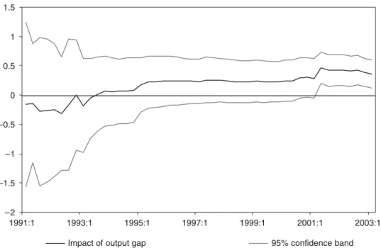
The information in the output gap appears to have gained importance over time.10In particular, the output gap is about as significant as money growth in the post-1986 sample, but much less significant in the pre-1987 sample.
•
These findings are important in that they provide a formal indication of the information content of money for future inflation.4. A TWO-PILLAR PHILLIPS CURVE
In this section I present my interpretation of the ECB’s monetary policy strategy. I start from the hypothesis that the strategy must be based on, at least implicitly, a ‘two-pillar’ view of inflation. The task I face, therefore, is to construct a model for forecasting inflation in which money plays an integral and non-trivial role.
As a first step, it is useful to clarify my interpretation of the ECB’s view of the inflation process. This is difficult because the importance that the ECB has attached to money has evolved over time. In particular, the review of the monetary policy framework which the ECB announced in 2002 and which was completed in 2003 led to a reassessment of the role and importance of money (see Box 3 for greater detail).
Box 3. The ECB’s 2003 review of the monetary policy strategy In October 1998, the Governing Council of the ECB announced the main features of its monetary policy strategy, the core of which is a quantitative definition of price stability and a two-pillar framework for assessing the risks to price stability. After more than three years of experience, the ECB stated in 2002 that it would review the framework. The outcome of this evaluation was made public in May 2003. While it considered both the quantitative definition of price stability and the two-pillar framework, in the interest of brevity I focus here on the implications for the monetary pillar. Galí et al. (2004) contains a detailed analysis of the overall outcome of the review.
While the review does not say so explicitly, my interpretation of it is that the Governing Council decided to maintain, but to downplay, the monetary pillar (von Hagen and Hofman 2003). Three notable changes were made.
First, the Governing Council appeared to change, or at least clarify, the motivation for the monetary pillar. When the two-pillar strategy was first intro-duced, the ECB argued that, given the high degree of uncertainty under which policy is conducted, the two-pillar strategy ‘reduces the risk of policy errors
10
This is evidenced by the fact that the adjusted R-squared from, and the significance of the slope parameter in, the univariate regressions are systematically higher in the second sample.
caused by the overreliance on a single indicator or model. Since it adopts a diversified approach to the interpretation of economic conditions, the ECB’s strategy may be regarded as facilitating the adoption of a robust monetary strategy’ (ECB, Monthly Bulletin, November 2000, p. 45).
It went on to argue that a specific concern was the fact that the inflation process was so poorly understood. On the same page, it stated that ‘A reflection of the uncertainties about, and the imperfect understanding of, the economy is the large range of models of the inflation process . . . Many of these models capture important elements of reality, but none of them appear to be able to describe reality in its entirety. Therefore, any single model is necessarily incom-plete. As the set of plausible models is very broad, any policy analysis needs to be organised within a simplifying framework. The ECB has chosen to organise its analysis under two pillars.’
Thus, when it was initially announced, the ECB motivated the two-pillar strategy by appealing to the risks that could arise from putting too much faith in any single hypothesis of the price mechanism.
After the conclusion of the review, the ECB continued to emphasize that the two-pillar framework was intended to avoid an excessive reliance on a single conceptual model of inflation (ECB, 2003, p. 17): ‘Monetary policy faces uncertainties about the functioning of the economy. The ECB’s monetary policy strategy was designed with the aim of ensuring that no information is lost and that appropriate attention is paid to different analytical perspectives . . . The two-pillar approach is a means to convey the notion of diversification of analysis to the public and ensure robust decision-making on the basis of different analytical perspectives.’
However, following the review, the ECB’s motivation focused on the need to combine information with different time dimensions (ECB, 2003, p. 18; see also the quotes in Section 4): ‘Overall, the two-pillar approach provides a framework for cross-checking indications stemming from the shorter-term economic analysis with those from the monetary analysis, which provides information about the medium to long-term determinants of inflation.’
Moreover, in the summary article in the June 2003 Monthly Bulletin, it writes that: ‘The Governing Council . . . indicated that monetary analysis mainly serves as a means of cross-checking, from a medium to long-term perspective, the short- to medium-term indications coming from economic analysis’ ( p. 87).
Overall, it seems that the motivation for the two-pillar approach changed as a consequence of review.
Second, the Governing Council decided to adopt a new structure for the President’s Introductory Statement to the ECB’s monthly press conference by reversing the order in which the information coming from the two pillars is presented. Thus, it was decided that the statement henceforth would start with the broadly based economic analysis under the second pillar before turning to
the monetary analysis of the first pillar. One plausible explanation for this decision is that the economic analysis provides more information about the Governing Council’s view of near-term inflation pressures, and therefore about the likelihood of interest rate changes, than the monetary analysis. I therefore believe this signals a reduction of the importance attached to the monetary pillar. This is supported by the fact that since December 2003, the term ‘pillar’ is no longer used in the editorials of the ECB’s Monthly Bulletin, which contain a discussion of the Governing Council’s view of economic developments and its assessment of the need for interest-rate changes.
The third change concerns the reference value for money growth. While the Governing Council in the past had reviewed this on an annual basis, it decided to discontinue this practice. This decision reflected the fact that since the monetary analysis pertained to the medium to long term, there would presumably be little reason to consider updating the reference value on an annual basis.
Despite this, I believe that the ECB’s view is based on the following three propositions:
•
Monetary policy impacts on inflation with a lag. It is therefore important to give monetary policy a ‘medium-term orientation’ and to forecast inflation at the time horizon relevant for monetary policy.•
Inflation depends on many factors. In the short run, it is largely influenced by cost variables (in particular energy prices and wages), the output gap, import and food prices, taxes and changes in administratively set prices. In the long run, however, it is determined solely by monetary factors. In the time horizon relevant for monetary policy, both sets of factors play a role and the central bank therefore faces a non-trivial forecasting problem.•
To assess the outlook for inflation at the medium-term time horizon, it is helpful to decompose inflation into two components or pillars. The first pillar is intended to capture the monetary factors that are useful for forecasting the long-run evolution of the price level. The second pillar is intended to reflect the factors that are helpful for predicting short-run movements in inflation.Overall, this analysis suggests that the important conceptual difference between the pillars concerns the forecasting horizon that they apply to. This interpretation seems compatible with the ECB’s own statements. In particular, in discussing the outcome of its widely noted review of the framework, it writes:
‘The two pillars are: economic analysis to identify short- to medium-term risks to price stability; and monetary analysis to assess medium to long-term trends in inflation, given the close relationship between money and prices over extended horizons.’11
11
See ‘The outcome of the ECB’s evaluation of its monetary policy strategy’, ECB Monthly Bulletin, June 2003, pp. 79 – 92, in particular p. 79.
It goes on to state that:
‘The inflation process can be broadly decomposed into two components, one associated with the interplay between demand and supply factors at a high frequency, and the other connected to more drawn-out and persistent trends . . . The latter component is empirically closely associated with the medium-term trend growth of money.’12
Furthermore, in an overview article directed to the scholarly community, the ECB (2003, p. 18) writes about the two pillars that:
‘One aspect of this approach relates to the different time perspectives relevant to the analysis under the two pillars. This builds on the well-documented findings that long-term price movements are driven by trend money growth, while higher frequency inflation developments appear to reflect the interplay between supply and demand conditions at shorter horizons. Against this background, the broadly based economic analysis gives higher-frequency indications for policy decisions based on the assessment of non-monetary shocks to price developments and the likely evolution of prices over short to medium-term horizons. Monetary analysis and indices of monetary imbalances, on the other hand, provide information against which these indications can be evaluated and the stance of policy can be cross-checked from a longer-term perspective’ (emphasis in the original).13
Thus, there can be little doubt that the main difference between the two pillars pertains to the time horizon they are supposed to be relevant for. Next I propose a model of inflation that combines monetary and non-monetary factors in this spirit.
4.1. The empirical model
Box 4 spells out the central elements of the model and the inflation equation that I estimate. Below I provide a non-technical discussion.
Box 4. The model
This box spells out the empirical model in detail. First I consider the filter discussed in the text. Sargent (1979, ch. 11) studies a consumption function in which permanent income is determined according to this filter. He states that Muth (1960) shows that this filter is compatible with the assumptions about expectations formation made by Friedman (1956).
12 Ibid., p. 87. See also Box 2 on p. 90.
13
Interestingly, on the same page the ECB writes ‘[t]he medium to long-term focus of the monetary analysis implies that there is no direct link between short-term monetary developments and monetary policy decisions.’
Let xt denote the annualized quarterly growth rate of some series. The
smoothed or filtered series, , is then given by:
. (1)
I use this formula on xt series corresponding to M3 growth, µt; adjusted
money growth, 5t ≡ µt − ∆yt, where ∆yt denotes the growth rate of real GDP;
and inflation, πt. I refer to the resulting -series as ‘trend money growth’, ‘adjusted trend money growth’ or ‘trend inflation’. All series are measured on an annualized quarterly basis: inflation, for example, is thus measured as 4 × log ( pt/pt−1). The ‘smoothing parameter’, λ, is important in that ln(2)/λ
captures the time it takes for a permanent one-unit change in xt to lead to a
0.5 unit change in (Cogley, 2002, p. 103). In Sections 2 and 3, I assume that
λ= 0.075; in Sections 5 and 6, I estimate λ.
Turning to the model, let gt denote the output gap; εt denote a residual; and
let a superscript e denote an expected value. I start from a standard, reduced-form Phillips-curve equation:
(2) which states that current inflation depends on expected future inflation, past inflation and the once-lagged output gap. I use the Hodrick–Prescott filter to construct a measure of the gap. Since there is typically a time lag between movements in the output gap and movements in inflation, I assume a one-period lag.
The relative weights of past, αb, and expected future, αf, inflation in the determination of inflation are of particular interest. While theory suggests that
αf ≈ 1, a number of studies from a range of economies typically estimate a much smaller value. I therefore test three hypotheses regarding these parame-ters: that the weights on the forward and backward-looking elements sum to unity (αf + αb = 1), that inflation is fully backward looking (αf = 0 and αb = 1) and that it is fully forward looking (αf = 1 and αb = 0).
Next, I assume that inflation expectations depend on :
, (3)
where a constant has been disregarded. Using equations (1), (2) and (3) and
assuming , Appendix 2 derives the TPPC, which integrates monetary
factors into a standard Phillips-curve equation and which constitutes my proposed interpretation of the ECB’s view of the inflation process:
πt = β1µt−1 + β2gt−1 + β3πt−1 + β4gt−2 + β5πt−2 + et, (4)
where β1 = αfλ, β2 = αg, β3 = (1 − λ + αb), β4 = −(1 − λ)αg, β5 = −(1 − λ)αb
and et = εt − ρεt−1 where ρ = 1 − λ. This equation is more complicated than a
traditional Phillips curve, but has a straightforward interpretation. xt* xt* =λxt ( ) *+ −1 λxt−1 xt* xt* πt α πf t α π α ε e b t g tg t , = +1 + −1+ −1+ xt* *, * *= µt 5 ort πt πte+1 *=xt−1 xt* *=µt
First, nominal money growth, my proposed representation of the first pillar, enters because it influences trend money growth, which in turn impacts on inflation expectations. The impact of money growth depends on λ, which captures how rapidly expectations change when money growth changes, and the extent to which inflation is forward looking, αf. Only if αf = λ = 1 is there
a one-to-one relationship between ( past) money growth and inflation.
Second, inflation depends on the output gap, which should be thought of as a shortcut for the many factors that enter in the second pillar. Needless to say, in a fully specified model it would be desirable to incorporate other elements capturing cost-push factors such as import and energy prices and changes in value added taxes.
Third, once-lagged inflation enters the equation for two reasons. Past inflation matters in the standard Phillips curve given by equation (2). The importance of this factor depends on αb. Furthermore, past inflation captures the importance of , which plays a role in determining as evidenced by the term (1 − λ). Fourth, gt−2 and πt−2 enter, provided that λ < 1. Thus, these variables appear
solely because of the assumed expectations-formation process. To see this most clearly, note that gt−2 and πt−2 do not enter the equation if λ = 1, in which case
expected future inflation is given by µt−1.
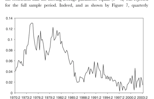
Fifth, the error term follows an MA(1) model with a coefficient that depends on λ. Of course, this results from the assumption that the εt-errors are serially uncorrelated, which need not be the case. Preliminary estimates suggested that the restriction that the moving-average parameter equals (1 − λ) was rejected for the full sample period. Indeed, and as shown by Figure 7, quarterly
µt*−1 µt*
changes of inflation display large negative first-order autocorrelation. This may be related to the way in which the price data are constructed or deseasonal-ized. I therefore do not impose the theoretical restriction that the moving-average parameter equals (1 − λ), but rather estimate it as a free parameter, ρ. Thus, I fit et = εt − ρεt−1.
It is important to note that the βi-parameters in the model depend on the underlying coefficients (αf, αg, αb, λ). To fit the model thus entails estimating these latter parameters rather than the βi’s. The model is estimated by writing equation (4) in state-space form and using the Kalman filter to evaluate the likelihood function.
In modelling the ECB’s view of the inflation process, I want to stay as close as possible to generally accepted macroeconomic building blocks. I therefore start from a standard Phillips-curve relationship that states that current inflation depends on expected future inflation, past inflation and the output gap.14 As in Section 3, I use
estimates of the output gap constructed using the Hodrick–Prescott filter. Since, empirically, there is typically a time lag between movements in the output gap and movements in inflation, I assume a one period lag. Before proceeding, I emphasize that Phillips curves are best seen as reduced-form relationships and therefore may shift if the policy regime changes.
An important aspect of Phillips-curve models concerns the relative weight of past and expected future inflation in the determination of inflation. While theory suggests that expected future inflation should play a dominant role, a number of studies from a range of economies indicate that past inflation may be more important. It is there-fore of interest to test the hypotheses that the weights on the forward and backward-looking elements sum to unity, that inflation is fully backward backward-looking and that it is fully forward looking.
To estimate the Phillips curve, the treatment of expected future inflation needs to be determined. The second building block of the model is therefore the assumption I make about how expectations are formed. If money growth is correlated with future inflation, as the data reviewed above suggest, then it should be correlated with inflation expectations. In fact, the ECB (2001, p. 42) has noted that one way in which money growth impacts on inflation is through induced movements in expected inflation:
‘High money growth may also directly influence inflationary expectations and therefore also price developments. Similarly, low monetary growth may lead to deflationary expectations and price developments.’15
14 Here I use the term ‘output gap’ in the older sense of the difference between actual and detrended real GDP (as opposed to the
more modern sense of the difference between actual real GDP and the level that would be observed if prices were perfectly flexible).
I therefore assume that trend money growth determines inflation expectations. This specification constitutes the main novelty of the paper and plays a critical role in the analysis that follows. It therefore warrants several comments.
First, while the notion that money growth affects inflation expectations may capture the spirit of the ECB’s view of the role of money in the inflation process, as suggested by the quote above, this assumption is arbitrary. However, the standard approach to modelling inflation expectations, that is to replace expected inflation by actual inflation and estimate the equation using statistical techniques appropriate for the resulting errors-in-variables problem as originally suggested by McCallum (1976), is also subject to important problems.16 It is, from this perspective, interesting that
several recent studies have modelled inflation using survey measures of expected inflation.17 It therefore seems appropriate to consider competing measures of
expected inflation in the euro area.
Second, since money growth does not enter the Phillips curve, it does not impact directly on inflation. One therefore wonders why it should impact indirectly through inflation expectations. To my mind, the assumption that money growth determines expected inflation should not be taken literally. The correlation between money growth and future inflation that has been established in the literature implies, how-ever, that money growth is correlated with expected inflation. I therefore interpret the ECB as believing that money growth captures the stance of monetary policy and the general state of aggregate demand, and that it therefore can be used as a proxy for expected inflation. The public, of course, may form their inflation expectations by looking at a broader set of variables and need not focus on money growth, although the fact that money growth and future inflation have been strongly correlated, for whatever reason, suggests that that would not be an unreasonable shortcut to take.
Third, the assumption that money growth impacts on inflation expectations gives rise to a direct channel from money to prices. Nelson (2003) argues that monetarist models hold that changes in money growth impact on prices indirectly through the level of aggregate demand and the output gap, and therefore do not require such a direct effect. By contrast, Galí (2003) appears to view such a direct mechanism as an important precondition for the use of the first pillar.
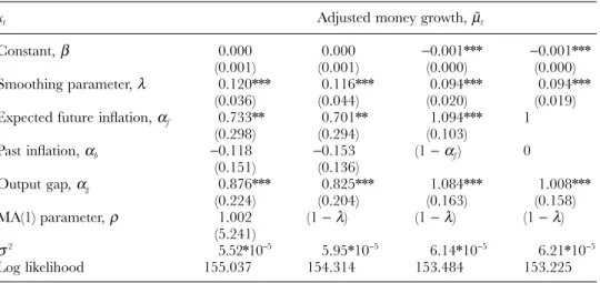
Fourth, while I interpret the ECB as believing that inflation expectations depend on current and past nominal money growth, I consider two other specifications. Since the quantity theory suggests that inflation is determined by the difference between money and real income growth, I also estimate the model using adjusted
16 In applied work, this approach is implemented by assuming that the expectation errors are uncorrelated with the regressors,
which are used as instruments. If the regressors involve variables that are not instantaneously observed (such as the output gap or recent inflation rates), this assumption leads to inconsistent estimates. While in principle this problem can be overcome by using lagged values of the instruments, in practice the information lags are unknown. Furthermore, this approach is silent on what factors determine inflation expectations. This modelling approach is thus also subject to arbitrary assumptions. 17
Adam and Padula (2003) study euro area and Roberts (1997 and 1998) investigates US data. Paloviita (2003) estimates forward-looking inflation equations on euro-area data, proxying expected inflation by OECD forecasts.
trend money growth. Moreover, since recent inflation is just as likely as money growth to be informative about future inflation, I also explore how well the model fits when trend inflation is used to model inflation expectations.
Fifth, since trend inflation depends on current inflation by construction, I lag it once to use it as a regressor in the inflation equation.
4.2. The two-pillar Phillips curve
Combining the Phillips curve, the expectations hypothesis and the definition of trend money growth discussed in Box 4, Appendix 2 shows how I can obtain a forecasting model for inflation, the ‘two-pillar Phillips curve’ (TPPC), that constitutes my pro-posed interpretation of the ECB’s view of the inflation process. That equation can be thought of as integrating monetary factors in a conventional reduced-form Phillips curve. The monetary analysis of the first pillar is captured by the assumption that expected inflation depends on trend money growth, while the economic analysis of the second pillar is captured by the output gap.
Before estimating the model, it is desirable to consider what would happen if the assumption that money growth can serve as a proxy for inflation expectations is wrong. How would this impact on the empirical results?
First, consider the case in which inflation expectations incorrectly are modelled using trend money growth. Since trend money growth in this case contains little information useful for forecasting inflation, one would expect the weight on expected future inflation to be small and insignificant and instead the weight on past inflation to be large and significant, given the fact that inflation is strongly autocorrelated. As I show below, however, the opposite is true: the weight on expected future inflation is generally much larger and more significant than the weight on past inflation.
Second, if money growth were not correlated with future inflation, one would expect that assuming that trend inflation rather than trend money growth determines inflation expectations would improve the fit of the model since current inflation is closely tied to trend inflation. The results below, however, consistently show that the model fits much worse if trend inflation is used instead of trend money growth. Overall, the results are difficult to reconcile with the notion that money growth does not contain incremental information that is useful for predicting future inflation.
5. FITTING THE DATA 5.1. Estimates
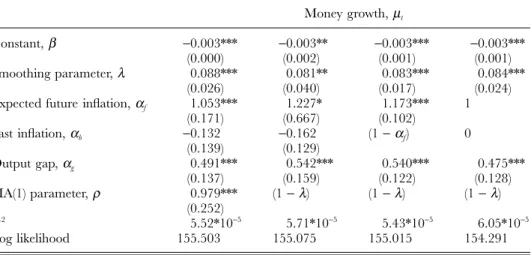
Table 1 provides estimates for the sample period 1971Q1–2003Q1. For the time being, I do not impose any restrictions on the degree to which expectations are forward or backward looking. The estimates in the first column, where I assume that money growth drives expected inflation, are quite encouraging. The smoothing
parameter is highly significant and estimated to be 0.089, which is close to the 0.075 value assumed by Gerlach (2003) and implies a half-life of 7.8 quarters. The estima-tion suggests that the weight on future inflaestima-tion is close to unity and is statistically significant. In turn, the weight on past inflation is 0.03 and highly insignificant. The parameter on the output gap is 0.55 and significant. Finally, the moving average parameter is 0.45. Since this is statistically significantly different from the value implied by the model (which is one minus the estimated value of the smoothing parameter: 1 − 0.089 = 0.911) there is some evidence against it.
In column 2 I consider the case in which expected future inflation is determined by adjusted money growth. The results are broadly similar to those just reviewed, with three differences. First, the point estimate of the smoothing parameter is larger, 0.13, implying a faster impact of money growth on expected inflation (half-life of 5.5 quarters). Second, the estimated impact of the output gap is 1.11 rather than 0.55. The reason for this is that adjusted trend money growth (which contains a moving average of past quarterly changes in income) and the output gap are negatively correlated. Third, the log likelihood is higher than before, implying that the model fits the data better when adjusted money growth is used as an explanatory variable for expected inflation.
As noted above, the most natural counter-argument to the notion that money is important in judging future price pressures is that any information that is contained in observations on recent money growth rates must surely already be embedded in recent inflation rates. If so, rather than focusing on recent and past money growth rates in assessing the ‘risks to price stability’, it would make much better sense to Table 1. Estimates of ππππt==== ββββ + ββββ1xt−−−−1 + ββββ2gt−−−−1 + ββββ3ππππt−−−−1 + ββββ4gt−−−−2 + ββββ5ππππt−−−−2 + et
where ββββ1==== ααααfλλλλ, ββββ2==== ααααg, ββββ3==== 1 −−−− λλλλ + ααααb, ββββ4==== −−−−(1 −−−− λλλλ)ααααg, ββββ5==== −−−−(1 −−−− λλλλ)ααααb, and et==== εεεεt−−−− ρρρρεεεεt−−−−1
Sample period 1971Q1 – 2003Q1
xt Money growth, µt Adjusted money growth, 5t Inflation, πt
Constant, β −0.003* (0.002) −0.002 (0.001) 0.001 (0.001) Smoothing parameter, λ 0.089** (0.035) 0.129*** (0.032) 0.224** (0.106) Expected future inflation, αf 1.041***
(0.243) 1.080*** (0.225) 0.922*** (0.228) Past inflation, αb 0.029 (0.172) 0.020 (0.182) 0.005 (0.232) Output gap, αg 0.553*** (0.141) 1.141*** (0.259) 0.628*** (0.146) MA(1) parameter, ρ 0.447** (0.191) 0.436** (0.194) 0.468*** (0.197) σ2 1.12*10−4 1.09*10−4 1.19*10−4 Log likelihood 403.631 405.521 399.641
Notes: Standard errors in parentheses.
concentrate on recent inflation rates. To assess this argument, I also consider the case in which expected future inflation is modelled as depending on trend inflation. The results, in column 3 of Table 1, are surprising. While most parameter estimates are similar to those obtained when inflation expectations are modelled as being tied to the growth rates of money or adjusted money, the fit of the model is clearly worse as evidenced by the sharp decline in the value of the likelihood function. The second major difference is that the smoothing parameter is much larger, 0.22, implying a half-life of 3.2 quarters.
5.2. Summary
In this section I have confronted the model for inflation arising from my proposed interpretation of the ECB’s monetary pillar with the data over the period 1971Q1– 2003Q1. While preliminary, these results are moderately encouraging in that the parameters are significant and take plausible values. The estimates of the extent to which inflation is backward looking are particularly interesting. In contrast to what one would expect from the literature, this parameter is numerically close to zero and statistically insignificant.
Next, I therefore refine the empirical work in two dimensions. First, I estimate the model for two sub-periods. I do so because it may be that while money growth played an important role in the high-inflation period in the 1970s and early 1980s, it lost its significance in the low-inflation environment of the 1990s. Gerlach (2003) presents evidence that suggests that the relationship between money growth and inflation in the euro area differed before and after 1992. The first subsample is the high-inflation period between 1971Q1 and 1991Q4, during which inflation averaged 7.1% per annum. The second is the low-inflation period 1992Q1–2003Q1, in which annual inflation averaged 2.3%.
The second refinement is that I investigate more closely some of the restrictions of the model. For instance, can I reject the hypothesis that the sum of the parameters on past and expected future inflation is unity or that inflation is entirely forward looking?
6. SUBSAMPLE ESTIMATES
6.1. Inflation in the euro area before 1992
In Table 2 I re-estimate the model on data ending in 1991Q4, assuming that nominal money growth determines inflation expectations. Column 1 shows the results when I do not impose the restriction on the moving-average parameter.18 Interestingly, in this
case I cannot reject this restriction and I therefore impose it. The results in column
2 indicate that the sum of the weights on the forward- and backward-looking components is marginally above unity, but not significantly so. I therefore introduce this restriction as well (column 3). However, in this case the smoothing parameter is not significantly different from zero. While the degree to which inflation is forward looking is only about 0.27, I impose the restriction that inflation is fully forward looking, which leads to a sharp fall in the likelihood function. Overall, I therefore conclude that the empirical model fits the data quite well in the first subsample when inflation expectations are modelled as depending on money growth and if inflation is assumed to be part forward, part backward looking.
Next, I turn to the case in which inflation expectations are modelled as determined by adjusted money growth. Interestingly, the results in Table 3 indicate that the model in this case fits the data better, as evidenced by the uniform increase in the value of the likelihood function. The value of the smoothing parameter is also con-sistently higher than in Table 2 (around 0.2 rather than 0.1), indicating a shorter half-life, and is more significant. As in the case of Table 2, the point estimates in column 1 suggest that I can impose the restriction on the moving average parameter and I do so in column 2. In column 3 I also impose the restriction that the sum of the weights on expected future inflation and past inflation is unity. This results in an estimate of the degree to which inflation is forward looking of 0.36, which is some-what higher than in Table 2. Finally, I restrict inflation to be fully forward looking, which again leads to a large fall in the value of the likelihood function.
In Table 4 I turn to the case in which inflation expectations are assumed to depend on trend inflation. The results are generally similar to those in Table 2, except that the fit of the equation is worse than before, as evidenced by the value of the likelihood Table 2. Estimates of ππππt==== ββββ + ββββ1xt−−−−1 + ββββ2gt−−−−1 + ββββ3ππππt−−−−1 + ββββ4gt−−−−2 + ββββ5ππππt−−−−2 + et where ββββ1==== ααααfλλλλ, ββββ2==== ααααg, ββββ3==== 1 −−−− λλλλ + ααααb, ββββ4==== −−−−(1 −−−− λλλλ)ααααg, ββββ5==== −−−−(1 −−−− λλλλ)ααααb, and et==== εεεεt−−−− ρρρρεεεεt−−−−1 Sample period 1971Q1–1991Q4 xt Money growth, µt Constant, β −0.003*** (0.000) −0.002*** (0.001) −0.001* (0.001) −0.004** (0.001) Smoothing parameter, λ 0.090** (0.036) 0.079** (0.037) 0.151 (0.100) 0.111*** (0.024) Expected future inflation, αf 0.492***
(0.139) 0.516*** (0.190) 0.269*** (0.085) 1 Past inflation, αb 0.681*** (0.066) 0.664*** (0.088) (1 − αf) 0 Output gap, αg 0.280** (0.117) 0.356*** (0.136) 0.306** (0.122) 0.673*** (0.178) MA(1) parameter, ρ 0.968*** (0.043) (1 − λ) (1 − λ) (1 − λ) σ2 1.13*10−4 1.16*10−4 1.21*10−4 3.02*10−4 Log likelihood 261.118 260.656 259.135 220.385
Notes: Standard errors in parentheses.