ELECTRONIC SUPPLEMENTARY MATERIAL FOR:
Understanding negative biodiversity-ecosystem relationship in semi-natural wildflower strips
Nadine Sandau; Russell E. Naisbit; Yvonne Fabian; Odile T. Bruggisser; Patrik Kehrli; Alexandre Aebi; Rudolf P. Rohr; Louis-Félix Bersier
Published in Oecologia
Appendix S1 - Experimental setup of the wildflower strips
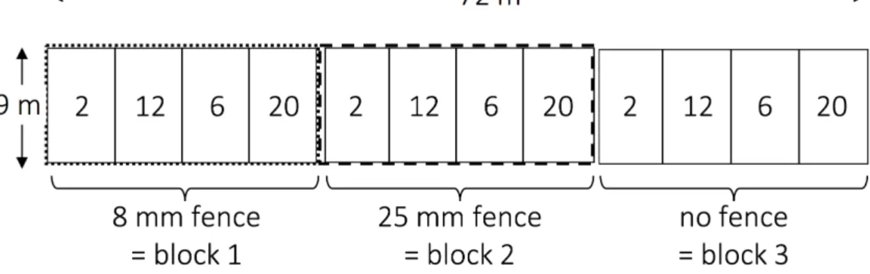
The Predator exclusion (PE) and predator and herbivore exclusion (PHE) were created with fences of mesh sizes of 25 mm and 8 mm respectively, were 1 m high and extended 0.2 m in the ground. The control plot was left unfenced. The design of the experimental wildflower strips, with the exclosure treatment and the sown species richness (SownS), is given in Fig. S1.1. In the PHE plots, we supplemented molluscicide mini-pellets containing 5% metaldehyde (Metarex®, De Sangosse) to control slug density. Treatment order was randomly designated to each field. For the substitutive design (each plant species added with the same proportion (Jolliffe 2000)) the seed density of the diversity mixtures was corrected to 1000 germinable seeds m-2 according to germination rates predicted by the commercial seed provider (UFA Samen Lyssach, Switzerland). If predicted germination success of a species was not equal to 100%, the amount of seeds was adjusted, i.e., proportionally more seeds were added. As other projects in our study system were concerned with the fauna (Fabian et al. 2012, 2013, 2014, Bruggisser et al. 2012), and because several studies suggested that weeding might increase invasion of undesired species (Wardle 2001, Roscher et al. 2009), we kept weeding to a minimum, removing only agricultural harmful weeds (Cirsium arvense and Rumex obtusifolius). In each field we also established an area with the original wildflower mixture, yet this data was excluded from the current analysis.
Fig. S1 Design of an experimental wildflower strip. Numbers within plots represent the sown species richness (SownS). The dashed and the dotted line represent the predator (PE) and the predator and herbivore (PHE) exclusion treatments, respectively
Appendix S2 – Lists of plant species Table S2.1 List of sown plant species
Plant family Plant species
Apiaceae Daucus carota L.
Pastinaca sativa L.
Asteraceae Achillea millefolium L. Anthemis tinctoria L. Centaurea cyanus L. Centaurea jacea L. Cichorium intybus L. Leucanthemum vulgare LAM. Tanacetum vulgare L.
Boraginaceae Echium vulgare L.
Caryophyllaceae Agrostemma githago L. Silene latifolia POIR.
Hypericaceae Hypericum perforatum L.
Caprifoliaceae Dipsacus fullonum L.
Lamiaceae Origanum vulgare L.
Malvaceae Malva moschata L.
Malva sylvestris L.
Papaveraceae Papaver rhoeas L.
Scrophulariaceae Verbascum thapsus L. Verbascum lychnitis L.
Table S2.2 List of external colonizer plant species recorded in the experimental plots
Plant family Plant species
Amaranthaceae Amaranthus retroflexus L. Chenopodium album L.
Chenopodium polyspermum L. Chenopodium sp.
Apiaceae Aethusa cynapium L.
Asteraceae Chamomilla recutita (L.) RAUSCHERT
Cirsium arvense (L.) SCOP.
Conyza canadensis (L.) CRONQUIST
Crepis biennis L.
Filaginella uliginosa (L.) OPIZ
Galinsoga ciliata (RAF.) S.F.BLAKE
Lactuca serriola L. Senecio vulgaris L. Sonchus arvensis L. Sonchus asper (L.) Hill Sonchus oleraceus L. Taraxacum officinale
Boraginaceae Myosotis arvensis (L.) HILL
Brassicaceae Brassica napus L.
Capsella bursa-pastoris (L.) MEDIK.
Sinapis alba L.
Campanulaceae Campanula patula L.
Caryophyllaceae Cerastium sp. Sagina apetala Ard. Stellaria media (L.) VILL.
Convolvulaceae Convolvulus arvensis L.
Equisetaceae Equisetum arvense L.
Euphorbiaceae Euphorbia helioscopia L. Euphorbia stricta L. Mercurialis annua L.
Fabaceae Lotus corniculatus L.
Medicago lupulina L. Medicago sativa L. Melilotus albus MEDIK.
Onobrychis viciifolia SCOP.
Trifolium pratense L. Trifolium repens L. Vicia hirsuta (L.) GRAY
Geraniaceae Geranium rotundifolium L.
Juglandaceae Juglans regia L.
Juncaceae Juncus bufonius L.
Juncus sp.
Lamiaceae Glechoma hederacea L.
Lamium amplexicaule L. Lamium purpureum L. Mentha arvensis L. Prunella vulgaris L.
Plant family Plant species
Onagraceae Epilobium sp.
Oenothera biennis L.
Orobanchaceae Orobanche sp.
Oxalidaceae Oxalis stricta L.
Plantaginaceae Chaenorhinum minus (L.) LANGE
Kickxia elatine (L.) DUMORT.
Kickxia spuria (L.) DUMORT.
Linaria vulgaris MILL.
Plantago lanceolata L. Plantago major L. Veronica persica Poir. Veronica serpyllifolia L.
Poaceae Agrostis stolonifera L.
Apera spica-venti (L.) P.BEAUV.
Arrhenatherum elatius (L.) P.BEAUV. ex J.PRESL & C.PRESL
Dactylis glomerata L.
Digitaria sanguinalis (L.) SCOP.
Echinochloa crus-galli (L.) P.BEAUV.
Elymus repens (L.) GOULD
Festuca sp. Holcus lanatus L. Lolium perenne L. Phleum pratense agg. Poa annua L.
Poaceae (undetermined) Setaria pumila (POIR.) SCHULT.
Triticum sp.
Polygonaceae Fallopia convolvulus (L.) A.LÖWE
Polygonum aviculare L.
Polygonum mite (=Persicaria laxiflora) Polygonum sp.
Rumex obtusifolius L.
Primulaceae Anagallis arvensis L.
Ranuculaceae Ranunculus repens L.
Rosaceae Potentilla reptans L.
Rubus sp.
Rubiaceae Galium album MILL.
Galium aparine L.
Salicaceae Salix alba L.
Salix caprea L.
Sapindaceae Acer pseudoplatanus
Scrophulariaceae Scrophularia nodosa L.
Solanaceae Solanum nigrum L.
Urticaceae Urtica dioica L.
Verbenaceae Verbena officinalis L.
Appendix S3 - Above-ground biomass estimations using leaf area index (LAI)
Biomass was predicted from the leaf area index (LAI): 27 measures per plot were taken using a LAI-2000 Plant Canopy Analyser from Li-COR Biosciences (Lincoln, Nebraska).
Additionally, we determined above-ground biomass in eight plots by cutting the above-ground biomass in five randomly selected 30 cm x 30 cm squares. As the Plant Canopy analyser cannot distinguish between leaf litter and senescent plant material, we did not sort the clipped samples into fresh biomass and dead biomass, instead we comprised all the plant material within the squares. Doing so we make sure to take into account plant material that was produced before the sampling event (Jenkins 2015). The plant material was bagged in paper bags and dried at 60°C until constant weight. To represent plot biomass, we calculated the average of the five samples.
We calibrated the clipped biomass and the LAI values by performing a regression analysis, which resulted in a Pearson product-moment correlation of 0.89. The linear relationship was used to predict plant biomass per plot in g*m-2 from the average LAI values.
Appendix S4 - Additional figures
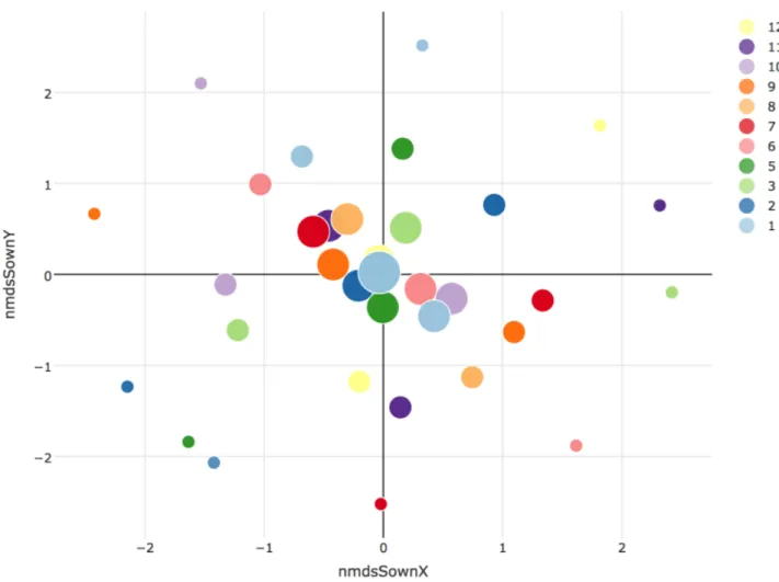
Fig. S4.1 NMDS ordination showing Sørensen dissimilarity among plots based on the sown plant assemblages. The colour schemes refer to different fields and the size of the symbol displays the number of species. Symbols located close together in the two-dimensional graph plots with similar composition. Note, that the three plots with the same diversity level within each field have the exact same NMDS sores. The distribution of the plots reflects the experimental design of the experiment, with constrained selection of the species so that they occur in similar frequencies at the same diversity level. In this way, the sown compositions appear evenly placed on concentric ellipses
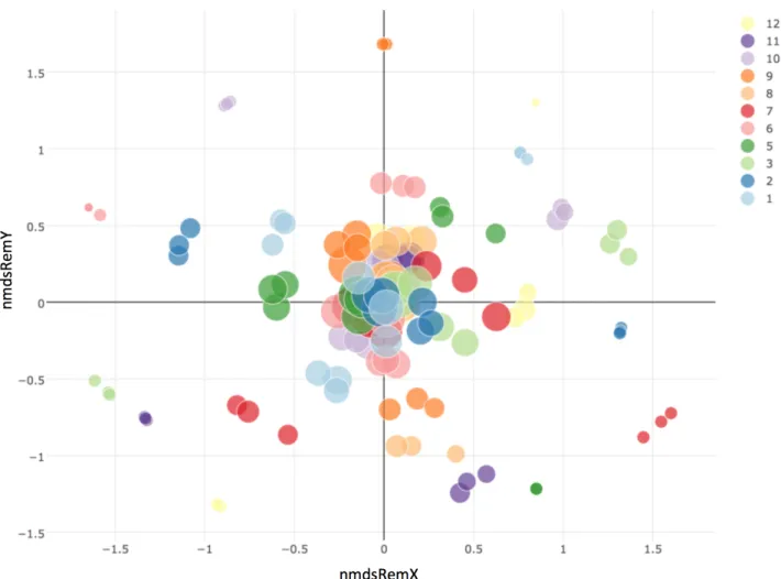
Fig. S4.2 NMDS ordination showing Bray-Curtis dissimilarity based on plant species abundance among plots for remaining plant species composition. The colour schemes refer to different fields and the size of the symbol displays above-ground biomass
Fig. S4.3 NMDS ordination showing Bray Curtis dissimilarity based on abundance plant species abundance among plots for colonizer plant species composition. The colour scheme refers to the 11 experimental fields and the size of the symbol displays above-ground biomass. We observe that plots from the same field tend to be clustered. We performed a Canonical Correspondence analysis on the same data, using field identity as explanatory variable, and found a highly significant effect of the latter (permutation test, p < 0.0001, analysis performed with functions cca and anova.cca from the vegan package; Oksanen et al. 2015)
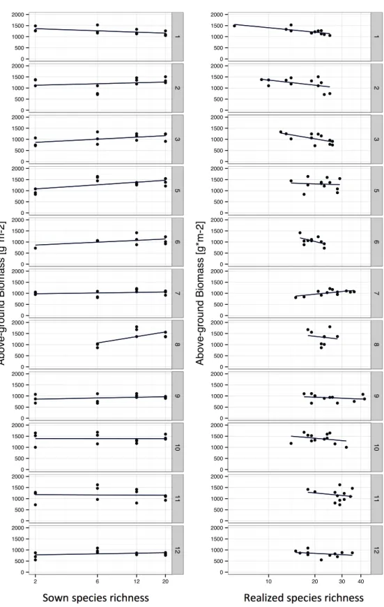
Fig. S4.4 Relationships of sown species richness (SownS) and realized species richness (S) and above-ground biomass within the different fields
0 500 1000 1500 2000 0 500 1000 1500 2000 0 500 1000 1500 2000 0 500 1000 1500 2000 0 500 1000 1500 2000 0 500 1000 1500 2000 0 500 1000 1500 2000 0 500 1000 1500 2000 0 500 1000 1500 2000 0 500 1000 1500 2000 0 500 1000 1500 2000 1 2 3 5 6 7 8 9 10 11 12 2 6 12 20
Sown Richness Levels
A bove-ground B iomass [g*m-2] 0 500 1000 1500 2000 0 500 1000 1500 2000 0 500 1000 1500 2000 0 500 1000 1500 2000 0 500 1000 1500 2000 0 500 1000 1500 2000 0 500 1000 1500 2000 0 500 1000 1500 2000 0 500 1000 1500 2000 0 500 1000 1500 2000 0 500 1000 1500 2000 1 2 3 5 6 7 8 9 10 11 12 10 20 30 40
Observed Species Richness
A
bove-ground
B
iomass
Appendix S5 - Results of the initial a priori piecewise structural equation model
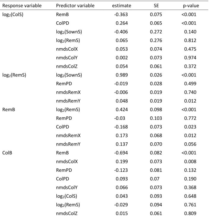
Table S5 This model gives all a priori relationships tested (see Table 3 and Fig. 7 for the final model). Biomass of the remaining sown species (RemB) and of colonizer species (ColB) are the response variables of interest. Variables: ColPD = phylogenetic diversity of colonizers; RemPD = phylogenetic diversity of remaining sown species; SownS = sown species richness; RemS = richness of remaining sown species; nmdsColX, -Y, and -Z = 1st, 2nd, and 3rd axes for composition of colonizers; nmdsRemX, -Y = 1st and 2nd axes for composition of remaining sown species
Response variable Predictor variable estimate SE p-value
log2(ColS) RemB -0.363 0.075 <0.001 ColPD 0.264 0.065 <0.001 log2(SownS) -0.406 0.272 0.140 log2(RemS) 0.065 0.276 0.812 nmdsColX 0.053 0.074 0.475 nmdsColY 0.002 0.073 0.974 nmdsColZ 0.054 0.061 0.372 log2(RemS) log2(SownS) 0.989 0.026 <0.001 RemPD -0.019 0.028 0.499 nmdsRemX -0.006 0.019 0.740 nmdsRemY 0.048 0.019 0.012 RemB log2(RemS) 0.424 0.098 <0.001 RemPD -0.03 0.103 0.772 ColPD -0.168 0.073 0.023 nmdsRemX 0.173 0.068 0.012 nmdsRemY 0.137 0.070 0.056 ColB RemB -0.694 0.082 <0.001 nmdsColX 0.199 0.073 0.008 RemPD -0.123 0.081 0.132 ColPD 0.093 0.07 0.190 nmdsColY 0.066 0.073 0.368 log2(ColS) 0.043 0.093 0.648 log2(RemS) -0.029 0.094 0.761 nmdsColZ 0.015 0.061 0.809
Appendix S6 - Details of model selection results
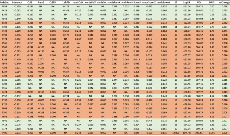
Table S6 The table gives all models with a DAIC ≤ 6. Models with an orange background were not selected as they are more complex version of models with lower AIC. Variables: ColS = species richness of colonizers transformed); RemS = species richness of remaining sown species (log2-transformed); ColPD = phylogenetic diversity of colonizer species; RemPD = phylogenetic diversity of remaining sown species; nmdsColX, nmdsColY, and nmdsColZ = 1st, 2nd, and 3rd NMDS axes for the composition of colonizer species; nmdsRemX and nmdsRemY = 1st and 2nd NMDS axes for the composition of remaining sown species; SownS = sown species richness (log2-transformed); nmdsSownX and nmdsSownY = 1st and 2nd NMDS axes for sown composition. Note that the exclosure treatment was included in all models
References
Bruggisser OT, Sandau, Blandenier G, Fabian Y, Kehrli P, Aebi A, Naisbit RE, Bersier L-F (2012) Direct and indirect bottom-up and top-down forces shape the abundance of the orb-web spider Argiope bruennichi. Basic App Ecol 13:706–714
Fabian Y, Sandau N, Bruggisser OT, Aebi A, Kehrli P, Rohr RP, Naisbit RE, Bersier L-F (2013) The importance of landscape and spatial structure for hymenopteran-based food webs in an agro-ecosystem. J Anim Ecol 82:1203–1214
Fabian Y, Sandau N, Bruggisser OT, Aebi A, Kehrli P, Rohr RP, Naisbit RE, Bersier L-F (2014) Plant diversity in a nutshell: testing for small-scale effects on trap nesting wild bees and wasps. Ecosphere 5:art 18
Fabian Y, Sandau N, Bruggisser OT, Kehrli P, Aebi A, Rohr RP, Naisbit RE, Bersier L-F (2012) Diversity protects plant communities against generalist molluscan herbivores. Ecol Evol 2:2460–2473 Jenkins DG (2015) Estimating ecological production from biomass. Ecosphere 6:art49
Jolliffe P (2000) The replacement series. J Ecol 88:371–385
Roscher C, Schmid B, Schulze ED (2009) Non-random recruitment of invader species in experimental grasslands. Oikos 118:1524–1540
Wardle DA (2001) Experimental demonstration that plant diversity reduces invasibility - evidence of a biological mechanism or a consequence of sampling effect. Oikos 95:161–170