HAL Id: cea-02491644
https://hal-cea.archives-ouvertes.fr/cea-02491644
Submitted on 26 Feb 2020HAL is a multi-disciplinary open access archive for the deposit and dissemination of sci-entific research documents, whether they are pub-lished or not. The documents may come from
L’archive ouverte pluridisciplinaire HAL, est destinée au dépôt et à la diffusion de documents scientifiques de niveau recherche, publiés ou non, émanant des établissements d’enseignement et de
impulsive loadings
D. Guilbaud
To cite this version:
D. Guilbaud. Damage plastic model for concrete failure under impulsive loadings. COMPLAS 2015 -XIII International Conference on Computational Plasticity Fundamentals and Applications, Sep 2015, Barcelone, Spain. �cea-02491644�
DAMAGE PLASTIC MODEL FOR CONCRETE FAILURE UNDER
IMPULSIVE LOADINGS.
DANIEL GUILBAUD*a,b *a
Commissariat à l’énergie atomique et aux énergies alternatives (CEA) DEN, DANS, DM2S, SEMT, DYN, 91191 Gif-sur-Yvette Cedex, France
*b
Institute of Mechanical Sciences and Industrial Applications (IMSIA), UMR 9219 CNRS-EDF-CEA-ENSTA,
Université Paris Saclay, 828 Boulevard des Maréchaux, 91762 Palaiseau Cedex, France Email: [email protected]
Key words:Concrete, Plasticity, Damage, Impact.
1 INTRODUCTION
The IRIS 2012 benchmark [1] was devoted to compare various modelling of impact on reinforced concrete slabs. Its aim was to improve the methods used and to provide guidance to assess the integrity of structures impacted by missiles.
During this benchmark, it appeared that damage plastic models developed in commercial software worked reasonably well to predict structural damage. This is the reason why a 3D constitutive model of this type, named DPDC (Damage Plastic Dynamic Concrete), was elaborated and introduced in EUROPLEXUS, a general finite element code for fast transient analysis of structures jointly developed by the CEA and the European Commission (EC – JRC ISPRA) and other partners of whom EDF. The model developed for industrial purposes should have been robust, efficient and easy to use. It was freely inspired by [2] whose model presents a sound theoretical basis and a reliable calibration procedure.
After a short theoretical overview of the model, numerical implementation and calibration procedure are succinctly described, and then comparisons with tests are presented.
2 THEORETICAL OVERVIEW OF THE CONCRETE MODEL
DPDC is an isotropic triaxial damage-plastic model. The plastic part is based on the effective stress and the damage part is based on total strain deformation measures. This kind of concrete model is widely used because plasticity and damage are simply coupled which mathematically leads to a well posed problem [3]. Furthermore, calibration procedure of parameters is easy to deal with. In the following sections, the great features of plastic and damage parts are specified and then strain rate effect is introduced to complete the model.
2.1 Plasticity model
The plasticity model is formulated in a 3D framework with a pressure sensitive shear (failure) convex surface, a hardening cap to close the yield surface on the compression axis and a non-associated plastic flow to control volume expansion. The yield surface is the product of three functions:
1, ' ,2 , '2 1, c m 1 c 1,
f J J J J F J F J (1)
where
Fcm describes the compressive meridian,
is the Willam-Warnke function,
Fc is the cap function and its hardening parameter,
J1 is the first invariant of the effective stress,
J’2 is the second invariant of the deviatoric effective stress,
is the Lode angle defined with J’2 and J’3.
Isovalue 0 represents the yield surface. Concrete behavior is elastic as long as stress state is strictly inside the surface (i.e. f < 0). The behavior becomes plastic if stress state reaches the surface (i.e. f = 0).
Plasticity is non-associative and g, the plastic potential, is defined by the stress space gradient where 𝑐𝑝 is a coefficient to reduce dilation when f /J1 0:
1 2 1 2 ' ' p J J g f f f c J J σ σ σ σ (2)
The shear failure function is defined along the compression meridian and only depends on the first stress invariant J1:
1 / ' 1 1 1 ' 2 / ' c p o r c c m c o r c c c J J F J f J k f (3) where J1orc, J’2orc, kc and pc are material parameters of the model defined for J1 < 0 and J1 > 0 .
A similar expression is used to define the extension meridian Fem(J1) and finally e(J1), the
eccentricity parameter, which is the ratio Fem(J1)/ Fcm(J1) used to calculate the
Willam-Warnke function [4]:
2 2 2 2 1 2 2 2 2 1 c o s 2 1 4 1 c o s 5 4 , 4 1 c o s 2 1 e e e e e J e e (4)This function gives the shape of the failure surface: (J1,)Fcm(J1). Its sections in
deviatoric planes transitions from an equilateral triangle (when J1 = 0) to a circle when the
pressure increases.
Concrete behavior is modeled by the product of failure and cap functions. The cap allows the simulation of pore compaction in order to control volumetric strain. It is described by a two-part function [5]. In traction and for low confining pressures, the function is equal to one. For higher confinement, it describes a part of an ellipse:
2 2
1, 1 1 / ( )
c
is the value of J1 at the intersection between the failure surface and the cap surface.
Geometrically, X( is the value of J1 at which Fc cuts the pressure-axis and it depends of the
cap ellipticity ratio Rcap:
( ) c a p c m( )
X R F (6)
The cap depends on the isotropic hardening parameter which determines the size of the cap. It is controlled by the plastic volumetric strain p
V
according to the following law [5]:
2
1 0 2 0 1 D X X D X X p V W e (7)where W, X0, D1, D2 are cap surface parameters. 2.2 Damage model
The damage formulation models two phenomena: strength and Young’s modulus reduction. In this model, damage is isotropic and controlled by a scalar damage parameter 𝑑. Resulting stress tensor is expressed as follows:
1 d
v p
σ σ (8)
Where v p
σ is the stress tensor after it is updated by the plasticity or viscoplasticity (defined later in 2.3). The damage parameter ranges from 0 to 1 and increases as damage accumulates from d 0 for no damage to d 1 for complete damage.
Damage initiates with plasticity when stresses are on the shear failure (and not on the cap). In order to capture unilateral effect, the parameter d is expressed via two different formulations, respectively called brittle and ductile damage, that use the level of stress triaxiality Tx defined as: Tx J1 / 3J '2 where Tx equals 1 in tension, 0 in pure shear and -1
in compression.
It is assumed that brittle damage accumulates in tension (i.e. Tx 0 ). It depends on the maximum principal strain m a x by mean of an energy-type term:
2
b
m a x
E
.
Brittle damage accumulates as soon as the failure surface is reached. This hypothesis defines the initial threshold 0
b
which was previously equal to 0:
0 m a x
b
in itia l
E
(11)
where the subscript initial stands for “when the failure surface is reached for the first time”. Then, brittle damage accumulates as long as the stresses are on the shear failure surface
and the increment of b
is positive: 0 b m a x E (12)
where m a xis the maximum principal strain increment.
On the contrary, ductile damage accumulates when the pressure is compressive ( Tx 0). It is driven by an energy-type term d
where is the strain tensor:
: d
d
v p (9) Ductile damage accumulates as soon as the shear failure surface is reached where plastic
volume strain is dilative (damage does not initiate on the cap where plastic volume strain is compactive). This hypothesis defines the initial threshold 0
d
which was previously equal to 0:
0 : d in itia l v p (10) Then, ductile damage accumulates with energy increment v p: related to the strain
increment as long as the shear failure surface is reached.
Note that an incremental definition of the thresholds has been chosen to follow more closely non radial loadings.
When becomes greater than its non-null value at previous time step, damages accumulate according to the following function:
0
( m a x/ ) (1 ) / (1 A ) 1
d d B B B e (13)
For each kind of damage, A and B are two shape parameters that depend on material properties and element size. B controls the initial slope of the d curve and A the surface under the curve. To maintain constant fracture energy regardless of element size [6], A depends on the element length (the cube root of the element volume) and the fracture energy term Gf that
depends on damage formulation, brittle or ductile.
In this model, to avoid numerical difficulties (mesh tangling …) it was chosen to use
m a x 0 .9 9 9
b
d for brittle damage. For ductile damage, to simulate the diminution of damage
with confinement (whenTx 1), the expression:
1 .5 m a x m in 0 .9 9 9; 1 /
d
x
d T is used.
The previous definition of brittle and ductile damage shows that the behavior of concrete is discontinuous for Tx 0. To mitigate this, a transition zone is introduced for ductile damage. When 1 Tx 0, B and Gf are continuous functions of Tx:
m in (1, ( ) )
b r it b r i p w r t t c x d u c B T B B B (14)
m in (1, ( ) )
f fb r it fb r p w r c t t u i x fd c G T G G Gwhere pwr, Brit and Bduct are parameters of the model.
This way, damage evolves from a ductile-type when Tx 1 to a brittle-type whenTx 0. Nevertheless, the transition is not completely smooth because damage threshold definitions are different.
To reduce pressure wave induced by sudden crack closure, fcc function is introduced to model gradual crack closure according to: fc c M in(1,M a x(Tx,0 )). This way, unilateral effect is complete only if Tx 1 (for at least uniaxial compression or more confined stress states) even if the mean compressive stress needed to close crack is generally lower than f’c the uniaxial compressive strength of concrete.
Now, a new damage parameter b c
d is introduced. This parameter is identical to the brittle
damage b
d when the pressure is tensile (Tx 0 ) and it is equal to zero if Tx 1:
(1 )
b c b
c c
d f d (15)
The damage parameter applied to the viscoplastic stresses is equal to the current maximum of the ductile or brittle with crack closure damage parameters:
m a x ( d, b c)
d d d (16)
Thus, there is no sharp transition between brittle and ductile damage unless in case of loading / unloading conditions leading to a switch between ductile and brittle formulations.
2.3 Strain rate effect model
Experiments show an increase of concrete strength as strain rate increases, both in tension and in compression. In this model, strain rate effects affect plasticity which is replaced by viscoplasticity, damage surface and fracture energy formulation.
The viscoplastic formulation is an extension of the commonly used Duvaut-Lions model described by Simo in [7]. He postulated that the viscoplastic strain rate is given by:
1 : / v p v p e p C where he introduced the “fluidity parameter” (physically, it is a time constant which could be related to the time a crack needs to propagate), e p
is the elastoplastic stress, v p
the viscoplastic strain, and C the hook tensor.
By using an implicit backward Euler algorithm to integrate the viscoplastic stress rate:
: : /
v p v p v p p
C C
one obtains the first order accurate formulae:
1 ( ( : 1) 1) / ( )
v p v p p
n n C n t n t
(17)
where t is the time step and n
Now, it is easy to find out the two limiting situations:
the static one when 0 , nv p1 np1 , so the inviscid plastic case is recovered,
the fast transient one when , 1 : 1 1
v p v p tr ia l
n n C n n
, so the elastic case is obtained.
Then, according to Murray, the model’s flexibility in fitting high strain rate data is improved by allowing the fluidity coefficient to vary with strain rate according to the generic expression below:
0( ˆ / ˆ0)
n d
t
(18)
where t0, n, ˆ0are input parameters and ˆd a measure of the deviatoric strain rate defined as
follow:
2
2
2 2 2 2 x x v yy v z z v x y yz x z ˆ ˆ ˆ ˆ εd 2 / 3 ε ε ε ε ε ε ε ε ε (19) where: ˆεv 1 / 3 ε
x x εyy εz z
Two distinct fluidity parameters are used: these are the fluidity parameter in uniaxial tensile stress t and uniaxial compressive stress c, each defined according to equation (18), but with different input parameters.
Due to the use of a transition zone in the ductile range, ductile fluidity parameter is defined according to:
m in (1, ( x )p w r c)
c t d t T (20)Finally, the fluidity parameter used in equation (16) is given by:
(1 H T( x)) d H T( x) b
where H is the Heaviside function.
In order to limit strain rate effect at high strain rates (typically when εˆ 1 00), the user has
to put a limit o v e r at the overstress. The overstress reads: o v e r Eˆε , meaning that the fluidity parameter is bounded.
With viscoplasticity, the initial damage threshold is delayed as follow:
'
0 0(1 Eεˆ0 0 / 0)
(22)
It is clear from equation (22) that initial threshold becomes greater as effective strain rate increases, and then damage initiation is effectively delayed.
The fracture energy is increased by a function of the strain rate effects according to the expression below:
1 εˆ / 0
v p f f G G E (23) 3 NUMERICAL IMPLEMENTATIONThe plastic part of the stress evaluation algorithm is based on the standard split into an elastic predictor and a plastic corrector using the cutting plane algorithm. Generally, a few iterations are used to obtain convergence if the strain increment is small. When strain rate effect is important, (about greater than 10 per second) it is no longer the case and then an automatic subincrementation is mandatory. In this case, damage is calculated at the sub increment level to avoid large damage increment.
The tritraction vertex needs a special treatment to project the stress on it. On the opposite, near the interaction of the cap with the hydrostatic axis, another treatment is needed to avoid finding J1 outside the cap surface. For this purpose, in equation (1), J '2 is no longer defined
like a function of J1 but the contrary.
Another special case is encountered with the displacement of the cap surface when the volumetric plastic strain vp asymptotically reaches the limit W. When this happens
numerically, the cutting plane algorithm no longer converges because the plastic correction becomes too low. As in the regime of full compaction, the yield surface follows the stress state, the hardening parameter is sought as the solution of equation (1) by a Newton Raphson scheme initialized with its previous value. The Lagrange’s multiplier is then deduced after vp is calculated with .
4 CALIBRATION PROCEDURE
The parameters for the compression meridian and the extension meridian are fitted as follow: When the pressure is tensile (J1 > 0), the failure surface is supposed to be given by
Rankine’s criteria. So, in this region, each meridian is a line segment and all the parameters of equations (3) are known and depend of f’t/f’c only. When the pressure is compressive, parameters are obtained with the following assumptions: - the meridians are continuous and differentiable at J1 = 0, - the uniaxial compression and a higher compressive point (J1hc,
2
' h c
J ) belong to the compressive meridian, - the biaxial compression belongs to the compressive meridian and lastly, after a very high compressive pressure (J1he = 100f’c) is
reached, compressive meridian and extension meridian have the same value. Finally, the data needed are: f’t/f’c, f’bc/f’c (=1.16 according to Kupfer’s results [8]), J1hc, J '2h c . This fit
matches in the range: 0 .0 6 f ' /t f 'c 0 .1 1 that corresponds to concrete grades from C20 to C80.
Cap surface parameters W, X0, D1, D2 can be deduced from pressure density curves
measured in hydrostatic compression test [9]. X0 is the pressure at which compaction begins,
W is the maximum plastic volume compaction and D1, D2 are two shape parameters that can
be deduced from the test by fitting the volumetric stain occupied by porosity of concrete:
21 0 2 0
ln (p o r o /W ) ln (W p) /W D (X X ) D (X X )
Knowing that volumetric strain compaction is found to initiate at f ' / 3c in uniaxial
compression, an approximation of Rcap is given by: 3 (X0 f ' ) /c f 'c.
The brittle fracture energy Gfbrit depends of f’c and maximum aggregate size according to CEB [10]. Due to lack of data, ductile fracture energy Gfduct is set 100 times Gfbrit. Brit and Bduct are parameters of the model fixed respectively as 0.1 to have the function (1-d) with a steep descent, and 100 to have the function (1-d) with a flat top.
Fluidity parameters are found by running numerous iterative calculations at the element level to retrieve the Dynamic Increase Factor specifications established by the CEB. Overstress coefficients are about 2/3 f’c.
5 COMPARISON WITH EXPERIMENTAL RESULTS
To validate the model, three kinds of tests have been carried out. The first kind was benchmarks at the element level for simple state of stress (traction, bi-traction, compression, bi-compression, pure shear …) with loading/unloading conditions. Due to lack of space here, these tests are not presented. The second kind of tests was benchmark at the specimen level, two of which are presented here: a Brazilian test and an unconfined compressive test. The last kind of test was conducted at structural levels: the first one deals with impacted beams, the second one simulates the perforation of a slab.
For all simulations, finite elements were 8 node solid elements with reduced integration (only one integration point). In simulations, volumetric strain appeared to be the best indicator of crack opening, so it was used to visualize crack pattern. Furthermore, it was also used to erode potentially distorted elements, the criteria being the maximum volumetric strain allowed: 0.1 in the case of the beams and 0.2 in the case of the slab.
5.1 Tests on concrete cylinders
Two tests on concrete cylindrical specimens are simulated: one in tension and one in compression along the vertical axis.
5.1.1 Brazilian test
The test in tension was a Brazilian one in which a vertical compressive load was applied diametrically to a disk specimen by mean of two thin strip bearings between the sample and the steel plates. The sample was a 7 cm diameter, 7 cm long cylinder made of ordinary
concrete with f’c=30 MPa and a maximum aggregate size of about 1 cm.
In the simulation, failure occurred along the vertical loading axis (figure 1). The crack firstly initiates at the disk center zone. Damage initiate in the ductile transition zone mentioned in 2.2 and due to the increasing triaxiality that became positive in the loading plane, brittle damage initiated and expanded rapidly towards the bearing strips (other cracks that can be seen on figure 1 appeared later).
According to the elasticity theory, the maximum vertical tensile stress is located at the center point of the disk specimen, and can be calculated by σt=2P/πDB where P is the load, D is the diameter, and B is the length of the specimen. The simulation gave σt= 4 MPa to be compared to 3.0 MPa. The difference is attributed to the strain rate effect, the loading rate being 2 cm/s.
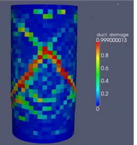
5.1.2 Unconfined compression test
The cylinder was a 16 cm diameter and 32 cm high sample made of ordinary concrete with
f’c=30 MPa and a maximum aggregate size of about 1 cm. The concrete cylinder was located
between two rigid steel plates, the bottom one was fixed and the other was compressing the sample at constant vertical velocity of about -6.7 mm/s. No slip was allowed between concrete and steel plates.
In the simulation, no strain rate effect was included because it seemed unneeded. It can be seen on figure 2 that ductile damage localized in two intersecting planes drawing an X pattern on the specimen. This failure mode is rather common for this kind of test.
Figure 1: Damage pattern for the Brazilian test Figure 2: Ductile damage pattern for the
unconfined compression test
5.2 Structural tests
In these tests, steel reinforcements are discretized with beam elements (3D steels in fig. 6, 7 and 10 are only for graphic representation). Perfect bond between steel and concrete is
assumed and realized by means of kinematic constraints because steel nodes and concrete nodes are not coincident. This requirement is demanded to deal with industrial cases that generally present complex reinforcement arrangement.
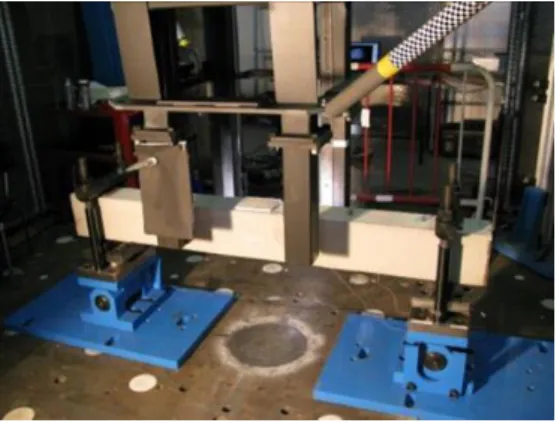
5.2.1 Drop-weight impacted beams
The influence of shear reinforcement of reinforced concrete short beams impacted by high-mass low-velocity striker is used here to see if the DPDC model is able to discriminate the two cases. The two beams were 0.2 m high, 0.15 width and 1.5 m long. The beams were reinforced with two 12 mm diameter high yield steel rebars at the bottom and with two 8 mm diameter high yield steel rebars at the top. Center of rebars are located 0.25 mm underneath the concrete surface. Shear reinforcement was made of 6 mm diameter mild steel frames, 0.2 m spaced from each other. The beams were supported to avoid rebound on the rotating bearings (see figure 3). The span of the beam was 1 m. A dropping tower equipped with a 103.65 Kg mass instrumented with a load cell was used to perform the tests. The striker was dropped from a height of 3.5 m to give an impact velocity of 8.3 m/s. The beams were made of ordinary concrete with f’c=33 MPa and a maximum aggregate size of about 1 cm.
Figure 3: View of a beam with its two rotating bearings instrumented with load cells.
Experimental crack patterns (figures 4 and 5) are compared to the plastic volumetric strain patterns drowned on figures 6 and 7. When shear reinforcement is present, the pattern is made of a major vertical crack surrounded by inclined shear cracks. This result is reproduced by the simulation satisfactorily. In the absence of shear reinforcement, a shear plug is formed under the striker. This failure mode is retrieved by the simulation even if the angle of the plug is overestimated so as the erosion.
For these failure modes, steel strains are reproduced correctly. In the first case, strains are localized in the middle of bottom rebars to form a plastic hinge in the beam, under the striker. In the second case, top rebars are severely bended under the impact zone, whereas bottom rebars acted as a membrane that retained the concrete plug.
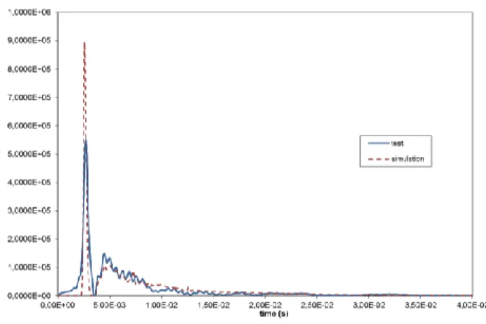
Impact load time histories are compared on figures 8 and 9. In the first configuration, the level of the load plateau following the peak can be well estimated by static limit analysis if the steel yield stress is increased by 10 %. This is in agreement with the order of magnitude of strain rate effect for rebars mentioned in [2]. Thus, this increased value has been used in the simulation.
Figure 4: Crack pattern at 5 ms
(beam with shear reinforcement)
Figure 5: Crack pattern at 500 ms
(beam without shear reinforcement)
Figure 6: Plastic volumetric strain pattern at the end
of the simulation (beam with shear reinforcement)
Figure 7: Plastic volumetric strain pattern at the end of the
simulation (beam without shear reinforcement)
Figure 8: Comparison of impact load time histories
(beam with shear reinforcement)
Figure 9: Comparison of impact load time histories
Finally, apart from the first load peak which is overestimated (maybe because the balsa pad used in the experiment was not modeled) the agreement is rather good for the two configurations.
With shear reinforcement, maximum beam deflection and residual deflection is reasonably well reproduced, the error being less than 10 % but post-pic oscillations are artificially damped out. Without shear reinforcement, the maximum beam deflection is over-estimated by 30 % whereas the residual deflection is slightly overestimated by only 10 %.
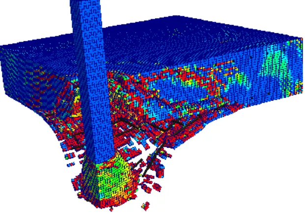
5.2.2 Perforation of a slab by a rigid impactor
This test is part of a benchmark devoted to the assessment of concrete model to deal with reinforced concrete members subjected to impact loadings [1].
In the experiment, a quasi-rigid projectile with a 47 Kg mass and a velocity of 135 m/s was launched against a 2 m square, 25 cm thick concrete slab. Concrete was characterized by a compressive strength of 61 MPa and a maximum aggregate size of 0.8 cm.
Rebars are made of high yield strength steel with an ultimate stress of 600 MPa. Their diameter was 1 cm and they were spaced out by 9 cm. No shear reinforcement was used. The slab is surrounded by a U-shaped corner plate and the whole is simply supported by means of log bearings.
Even missile buckling and slab cracking do not follow strictly the symmetry pattern, only a quarter of the shock configuration was discretized to save computation time, that’s why, boundary conditions of symmetry type were introduced for missile and slab.
Steel beam elements eroded when the strains reached the maximum elongation before necking appeared (ultimate limit of 20 %).
Figure 10: Plastic volumetric strain pattern at 10 ms
Plastic volumetric strain pattern is shown on figure 10 at the end of the perforation. Even if erosion of concrete elements seems too important, the failure mode is well reproduced: shear concrete plug pushed by the missile is well visible and, in the surrounding, shear cracks are present so as the scabbing of the concrete cover.
The residual velocity of the missile given by the simulation is 25 m/s, which is to be compared to an experimental value ranging between 35 m/s and 45 m/s.
12 CONCLUSIONS
The DPDC model is based on sound theoretical basis that has been briefly described here so as the calibration procedure. As shown in this paper, DPDC model has been verified at the specimen level on basic tests: a Brazilian test and an unconfined compressive test. Furthermore, it has been validated upon impact tests against reinforced members. Maximum and residual deflections of beams are reproduced so as impact load time histories. Damage patterns reproduce cracks satisfactorily. The first simulation of the perforation of a slab by a rigid missile gave a reasonable assessment of its residual velocity.
Nevertheless, some points needs to be improved:
First, at the beginning of hard impact, even if the impulse is well reproduced, the first peak load is overestimated and too narrow. This point needs special investigation.
Then, post-peak oscillations are damped out, probably because crack closure are not reproduced due to fully damage elements continuing to deform plastically or, when erosion is activated because research of auto-contacts is not activated. Also, extra work is necessary to try obtaining a better evaluation of shock induced vibrations.
Finally, as it can be seen on the simulations of the impacted beams, damage patterns are not symmetric but the meshes are. This illustrates the great sensitivity of these results to the mesh used in calculation although the Hillerborg’s method is used. In an attempt to mitigate this, a viscoplastic regularization of damage will be introduced instead of simply delaying damage by increasing the initial threshold.
REFERENCES
[1] Improving Robustness Assessment Methodologies For Structures Impacted by Missiles (IRIS_2012), Final report, NEA/CSNI/R(2014)5-ADD1 (2014).
[2] Y. Murray, Users’ manual for LS-DYNA Concrete Material Model 159, Publication Federal
Highway Administration FHWA-HRT-05-062, USA, (2007).
[3] P. Grassl, M. Jirasezk, Damage-plastic model for concrete failure, Int. J. of Solids and Structures 43 (2006), 7166-7196.
[4] K.J. Willam, E.P. Warnke, Constitutive model for Triaxial Behavior of Concrete, Concrete
Structures Subjected to Triaxial Stresses, International Association for Bridges and Structural
Engineering, Bergamo, Italy, May 1974.
[5] L.E. Schwer, Y.D. Murray, A three invariant smooth cap model with missed hardening, Int. J. for
Numerical and Analytical Methods in Geomechanics 18 (1994), 657-688.
[6] A. Hillerborg, M. Mooder P. Patersson, Analysis of crack formation and crack growth in concrete by means of fracture mechanics and finite elements, Cement and Concrete Research, 1976. [7] J.C. Simo, J.G. Kennedy and S. Govindjee, Non-smooth Multisurface Plasticity and
viscoplasticity. Loading/unloading Conditions and Numerical Algorithms, Int. J. for Numerical
Methods in Engineering 26 (198), 2161-2185.
[8] H. Kupfer, H. Hilsdorf, Behavior of concrete under biaxial stresses, J. of the American Concrete
Institute, 66-8, (1969), 656-666.
[9] S.J. Green, S.R. Swanson, Static constitutive relations for concrete. Air Force Weapons Laboratory (Technique Report N°. AFWL-TR-722), Kirtland Air Force Base, 1973.