HAL Id: hal-00777138
https://hal.archives-ouvertes.fr/hal-00777138
Preprint submitted on 16 Jan 2013
HAL is a multi-disciplinary open access
archive for the deposit and dissemination of sci-entific research documents, whether they are pub-lished or not. The documents may come from teaching and research institutions in France or
L’archive ouverte pluridisciplinaire HAL, est destinée au dépôt et à la diffusion de documents scientifiques de niveau recherche, publiés ou non, émanant des établissements d’enseignement et de recherche français ou étrangers, des laboratoires
Gigahertz laser resonant ultrasound spectroscopy for the
evaluation of transverse elastic properties of micrometric
bers
Denis Mounier, Christophe Poilane, Haithem Khelfa, Pascal Picart
To cite this version:
Denis Mounier, Christophe Poilane, Haithem Khelfa, Pascal Picart. Gigahertz laser resonant ul-trasound spectroscopy for the evaluation of transverse elastic properties of micrometric bers. 2013. �hal-00777138�
Gigahertz laser resonant ultrasound spectroscopy for the evaluation
of transverse elastic properties of micrometric fibers
Denis MOUNIERb,d,∗, Christophe POIL ˆANEc, Haithem KHELFAa, Pascal PICARTa,d aLUNAM Universit´e du Maine, Laboratoire d’Acoustique de l’Universit´e du Maine (LAUM), UMR CNRS
6613, Avenue Olivier Messiaen, 72085 Le Mans cedex 9, France
bLUNAM Universit´e du Maine, Institut des Mol´ecules et des Mat´eriaux du Mans (IMMM), UMR CNRS
6283, Avenue Olivier Messiaen, 72085 Le Mans cedex 9, France
cCentre de Recherche sur les Ions, les Mat´eriaux et la Photonique, (CIMAP Alen¸con), UMR6252
ENSICAEN-UCBN-CNRS-CEA, IUT d’Alen¸con, 61250 Damigny, France
dEcole Nationale Sup´erieure d’Ing´enieurs du Mans, rue Aristote, 72085 Le Mans cedex 9, France
Abstract
The cross section eigenmodes of micrometric cylinders were measured in the range of several tenth of MHz to about 0.5 GHz. The vibrations were excited using subnanosecond laser pulses. The cross section eigenmodes were simulated using finite element modeling in a 2D geometry. Using the method of resonant ultrasound spectroscopy, the vibration spectrum of an aluminum wire of diameter 33µm served to determine the transverse Young modulus and Poisson ratio with a precision of 0.7% and 0.3%, respectively. The calculated and measured frequencies of cross section eigenmodes were fitted with a precision better than 0.5% in the 50-500 MHz range.
Keywords:
fiber, laser ultrasonics, resonant ultrasound spectroscopy (RUS), finite element modeling, laser interferometry, cylinder, eigenmodes, Rayleigh modes, wave gallery modes, design of experiment (DOE)
1. Introduction
1
Resonant ultrasound spectroscopy (RUS) has been extensively used during the past two
2
decades to evaluate the elastic constants of various anisotropic solid materials with an
ulti-3
∗Corresponding author
mate precision [1–4]. From the measurement of the mechanical resonance frequencies of a
4
sample, the elastic constants of the material can be determined.
5
The PZT-RUS method, i.e. the RUS technique using piezoelectric transducers for both
6
the excitation and the measurement of vibrations, is the most widely used technique. The
7
optimum size of the sample for PZT-RUS is about 1 cm, but the technique can be used
8
for small samples whose dimensions are of the order of 0.5 mm with specially designed
9
transducers [3]. For such small samples, the RUS technique may require the measurement
10
of resonance frequencies up to 50 MHz [5].
11
However, even in the case of samples of several millimeters in size, contact forces between
12
the ultrasonic transducers and the sample may lead to spurious frequency shifts for the
13
resonance frequencies in addition to the widening of resonances [6–8]. The problem of
14
contacts comes up more and more crucial as the size of samples decreases.
15
The suppression of contact forces by using lasers for both the excitation and the detection
16
of vibrations results in getting sharp resonances, which is beneficial to the accuracy of
17
measurement [7, 8]. The excitation of vibrations can be carried out by using a periodic
18
laser modulation, whose frequency is swept over the required range [9]. Alternatively, short
19
laser pulses can be used to excite the vibrations of the sample. The advantage of the pulsed
20
method lies in the possibility of exciting simultaneously many eigenmodes over a very large
21
frequency range. The broad band excitation provided by short optical pulses is particularly
22
appropriate to the study of very small samples. The vibrations are measured in the time
23
domain and the eigenfrequencies are obtained from the Fourier transform of the measured
24
signal. The pulsed Laser-RUS method is preferable to determine the elastic constants of
25
small samples [7, 8, 10, 11] or to detect flaws in a small composite structure [12–15]. In this
26
paper, we present a pulsed LRUS technique applied to the evaluation of elastic constants of
27
micrometric fibers, whose diameters are in the range 5-50 µm. For such small dimensions,
28
the eigenfrequencies must be measured in the 0.05-1 GHz range.
29
The LRUS allows one to evaluate the elastic constants on a single fiber, in contrast
30
with indirect methods of evaluation [16]. From the evaluation of the elastic constants of a
31
unidirectional fiber composite, the elastic constants of the fibers are calculated. This indirect
method is based on specific assumptions about the nature of the reinforcing effect of fibers
33
in the polymer matrix. These assumptions may not be valid for all kinds of reinforced
34
polymers, so the application of this method may lead to erroneous results. Therefore, it is
35
is much more reliable to evaluate the elastic constants directly on a single fiber.
36
A direct evaluation of elastic constants of carbon fibers by a non-contact technique was
37
first achieved using the technique of laser picosecond ultrasonics [17]. The transverse elastic
38
constant C11 of carbon fibers was evaluated through the measurement of the time of flight of
39
acoustic pulses that propagate back and forth across a fiber diameter, which determines the
40
longitudinal acoustic velocity and then the C11 elastic constant. However, the evaluation of
41
the C44elastic constant, which requires the measurement of the transverse acoustic velocity,
42
could not be achieved because of the difficulty to generate and to detect picosecond transverse
43
acoustic waves.
44
Fibers are commonly used in reinforced polymers, such as glass or carbon fibers. The
45
interest of the method is great for anisotropic fibers (carbon and vegetal fibers) because
46
of the lack of reliable and accurate methods for the evaluation of the elastic constants of
47
fibers, in particular the elastic constants characterizing the transverse elastic properties.
48
The evaluation of the longitudinal Young modulus of fibers is generally carried out using
49
the tensile test method [18, 19]. But this method is impracticable to measure the transverse
50
elastic properties.
51
We illustrate the application of the LRUS method to the evaluation of the transverse
52
Young modulus and Poisson ratio of a micrometric aluminum wire. The evaluation of the
53
transverse elastic properties of fibers requires the excitation of the cross section eigenmodes.
54
In our approach, the propagation of guided acoustic waves along the fiber axis is neglected,
55
so the mechanical displacements are restricted to a plane perpendicular to the fiber axis.
56
The restriction in 2D of the cylinder vibrations results in a discrete vibration spectrum,
57
which is required for the application of the RUS method. In section 2, we will describe the
58
experimental method used to excite and detect cross-section modes of a fiber. In section 3,
59
we will present the method used to solve the inverse problem, which leads to the evaluation
60
of the transverse elastic properties of an aluminum fiber. We will also discuss the conditions
of validity RUS applied to a cylinder.
62
2. Measurement of ultrasonic vibrations
63
2.1. Laser ultrasonic setup
64
The irradiation of a cylinder with a laser pulse can excite many acoustic guided modes.
65
The propagation of guided modes along the cylinder axis is determined by the dispersion
66
relation ω(k), where k is the propagation wave vector along the cylinder axis and ω/(2π)
67
is the frequency of the guided mode. The dispersion relation determines both the phase
68
velocity vφ= ω/k and the group velocity vg = dω/dk of the guided mode.
69
Both the geometry of the laser spot focused on the cylinder surface and the duration
70
of the laser pulse determine the spectral range of guided modes that can be excited. If
71
the pump beam is focused to form a linear spot parallel to one of the generating line of
72
the cylinder, then a linear acoustic source will be formed and a cylindrical acoustic wave
73
propagating perpendicularly to the cylinder axis will be generated. Consequently, a linear
74
acoustic source parallel to the cylinder axis, which is very long compared to the fiber diameter
75
will favor the excitation of guided modes which very small wave vectors k ≈ 0, i.e. with
76
very large wavelengths λ = 2π/k compared to the fiber diameter. Moreover, such a linear
77
acoustic source will force the displacements in the directions perpendicular to the cylinder
78
axis and the displacements will be almost independent of the z-coordinate around the center
79
of the acoustic source.
80
Figure 1 shows the LRUS setup, which includes two parts: the first part is devoted to the
81
excitation of vibrations and the second part, the interferometer, serves to measure ultrasonic
82
vibrations. The vibrations of fibers are excited using a Q-switched Nd:YAG microchip laser
83
at 1064 nm from TEEM photonics whose pulses have a maximum energy of 10µJ and a
84
duration of 0.6 ns at a maximum repetition rate of 5 kHz. With a 0.6 ns pump pulse, it is
85
possible to generate vibrations up to the 1-2 GHz frequency range, which is sufficient to
86
excite many eigenmodes of a fiber whose diameter is in the 5-50 µm range.
87
The fibers are mounted on a 1 cm diameter plastic ring (Inset of Fig. 1, at the bottom
88
right). In order to excite acoustic waves which propagate mainly perpendicularly to the
Figure 1: Experimental setup of laser ultrasonic resonance spectroscopy (L-RUS) and support of the fiber. BS: beam splitter, PBS : polarizing beam splitter, VA: variable attenuator, λ/4: quarter-wave plate, λ/2: half-wave plate, M1, M2, M3, M4: mirrors, PZT: piezoelectric actuator, GD: ground potential.
fiber axis, the length of the pump spot must be much larger than the fiber diameter. The
90
pump laser is therefore shaped to form a narrow line, parallel to the fiber axis. By using a
91
cylindrical lens placed in the optical path of the pump beam, we obtain an elliptical spot
92
with dimensions 6µm × 100 µm at the fiber surface, with the main axis of the ellipse aligned
93
with the fiber axis (see left inset of Fig. 1). By a proper adjustment of the pulse energy with
94
an variable attenuator (not represented on Fig. 1), the vibrations of the fiber can be excited
95
in the non destructive thermoelastic regime [20].
96
For the measurement of radial ultrasonic vibrations, a stabilized homodyne Michelson
97
interferometer is used [20]. The probe beam at 532 nm is focused onto the fiber surface using
98
an aspherical lens (x20) having 8 mm focal length and 0.5 numerical aperture. The resulting
99
focused spot centered on the pump line has a diameter of about 2µm (inset of Fig. 1).
100
An incident probe power of 1-2 mW is sufficient to achieve a measurement sensitivity of
1 mV nm−1 on a metallic surface.
102
The optical interferometric signal is received by a high-speed photodetector with a
band-103
pass of 1 GHz. Using a digital oscilloscope with a band-pass of 3 GHz, the signals are
104
recorded in synchronization with the pump pulses during about 2 µs after the pump laser
105
pulse. Thanks to the averaging of 10 000 acquisitions, which necessitates a only two seconds
106
at the pulse repetition rate of 5 kHz, we obtain a detection threshold of about 5 pm for the
107
measurement of out-of-plane displacements, which is sufficient to detect the vibrations with
108
a satisfactorily signal to noise ratio.
109
The high frequency ultrasonic vibrations are superimposed to a slow and huge
displace-110
ment of the fiber; a displacements of about 5-10 nm which is probably induced by the sudden
111
expansion of the air in contact with the heated fiber surface, thus inducing the recoil of the
112
fiber. This slow drift of the signal is filtered out in order to magnify the high frequency
113
vibrations corresponding to the fiber cross-section eigenmodes. The vibration spectrum is
114
obtained with 0.5 MHz resolution by calculating the Fast Fourier Transform (FFT) of the
115
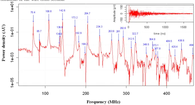
digitized signal (Fig. 2).
116
2.2. Vibration spectrum of an aluminum wire
117
The test sample is an aluminum bonding wire with 1% silicon, manufactured by
HER-118
AEUS [21]. With a scanning electron microscope (SEM), we measured the wire diameter
119
at several points of the wire. A mean diameter of (32.7 ± 0.1)µm was determined over a
120
length of 1 cm.
121
The ultrasonic measurements were made at several points each millimeter over a wire
122
length of 5 mm.
123
Figure 2 shows one of the measured vibration spectra of the aluminum wire. The inset
124
of Fig. 2 represents the high frequency ultrasonic component used to calculate the vibration
125
spectrum. Each eigenfrequency can be determined with an accuracy of about 0.5 MHz. For
126
each spectral line, the mean frequency and standard deviation were calculated from the
127
vibration spectra measured at different points of the wire. The standard deviations was
128
found of the order of the spectral resolution 0.5 MHz. The repeatability of the vibration
Figure 2: Eigenfrequency spectrum of an aluminum wire of diameter 32.7µm calculated from the signal shown in the inset, which shows the high frequency component of the recorded signal, corresponding to the vibrations of the wire cross-section.
spectra assesses the constancy of the wire diameter over a length of 5 mm.
130
The next step before determining the transverse Young modulus and Poisson ratio of the
131
aluminum wire is the identification of eigenmodes.
132
3. Evaluation of the transverse elastic properties of an aluminum fiber
133
3.1. Two-dimensional finite element modeling
134
In the following, we will focus our attention on k = 0 guided modes, whose displacements
135
are restricted within the xy-plane. From the experimental conditions depicted before, we
136
expect that the excited eigenmodes are mainly the k = 0 guided modes. We will refer to such
137
guided modes as cross-section modes. The eigenfrequencies of cross-section modes depend
138
only on the transverse Young modulus and Poisson ratio of the cylinder. Consequently,
139
from the measured eigenfrequencies, the transverse Young modulus and Poisson ratio can
140
be determined.
A 2D mechanical model of the aluminum wire is carried out. It is assumed that the
142
elastic properties are homogeneous and invariant by rotation around the fiber axis, i.e. the
143
mechanical properties of the material are transverse isotropic. Thus, the eigenmodes are
144
determined by: the cylinder diameter d, the Young modulus E, the Poisson ratio ν and
145
density ρ. The vibration eigenmodes of an aluminum wire are determined with the software
146
COMSOL Multiphysics. The mode shapes of the first 20 eigenmodes are illustrated in Fig.
147
3.
148
3.1.1. Nomenclature of modes
149
The guided modes of a cylinder are named according to the nomenclature of Silk and
150
Bainton [22]. The modes are labeled X(m, n) (or simply Xm, n as in Fig. 4 or Table 1)
151
where X = L, T, or F and m, n are positive integers. The letters L, T or F are the initials of
152
longitudinal, torsional and flexural modes, respectively. The number m of a X(m, n) mode
153
characterizes the rotational symmetry of the mode shape and n the ordering of the Xm
154
mode in the frequency scale. In cylindrical coordinates (r, θ, z), the ur and uθ components
155
of the displacement field vary according to the functions cos mθ or sin mθ, which means that
156
the mode shape is invariant after a rotation of 2π/m rad around the cylinder z-axis. The
157
longitudinal and torsional modes, which have both a rotational symmetry for an arbitrary
158
rotation angle around the cylinder axis have m = 0. The longitudinal and the torsional
159
modes are characterized by the displacements uθ = 0 and ur = 0, respectively. The modes
160
with m > 0 are flexural modes.
161
According to Victorov [23, 24], the cross-section modes belong to one of the two
cat-162
egories: the Rayleigh modes (R) or the Wave Gallery modes (WG). The Rayleigh modes
163
are flexural modes of the n = 0 series, which we denote more explicitly R(m, 0) instead of
164
F (m, 0). The Rayleigh modes series starts with the R(2, 0) mode, as the R(1, 0) mode is
165
the trivial Rayleigh mode corresponding to the translation of the cylinder along a radial
166
direction, having thus the frequency zero. The WG modes are denoted W G(m, n) instead of
167
F (m, n), with n > 0 and m > 0. The first longitudinal mode, denoted L(0, 1), is often called
168
the breathing mode. The first torsional mode is denoted T (0, 1). The L(0, 0) and T (0, 0)
modes are trivial modes with their eigenfrequency equal to zero.
170
The distinction between Rayleigh and some series of Wave Gallery modes will be useful
171
to consider in the perspective of mode identification, as all Rayleigh modes have significant
172
radial components ur and weak orthoradial components uθ at the surface of the cylinder.
173
On the contrary, the n = 1 series of Wave Gallery modes is characterized by weak radial
174
components compared to the orthoradial ones and the displacements are mainly concentrated
175
in the vicinity of the surface. The displacements for WG modes of the series n > 1 may
176
have very weak components at the surface. In contrast, for some particular WG modes (for
177
example see mode 12 in Fig. 3 and Table 1), the magnitude of the radial displacement
178
may be significant. Considering the correlation between the relative magnitude of radial
179
displacements predicted by the modeling and the amplitudes of the spectral lines may help
180
to identify the modes (cf. section 3.2).
181
The longitudinal modes L(0, n) and the torsional modes T (0, n) are not degenerate.
182
On the contrary, the m > 0 modes are two-fold degenerate. This property arises from the
183
existence of the two angular functions cos mθ and sin mθ, expressing the angular dependence
184
of a mode shape. The two degenerate mode shapes can be deduced from each other by a
185
rotation of π/(2 m) rad. If a fiber deviates a little from the circular symmetry, a degeneracy
186
lifting may occur. If the spectral resolution is sufficient, it could be possible to appreciate an
187
elliptical shape of the fiber cross-section. In the spectrum of Fig. 2, the absence of doublets
188
in the spectrum demonstrates the almost perfect circular cross-section of the aluminum wire.
189
3.2. Modes identification
190
The RUS technique requires the correct mode identification of each measured
eigenfre-191
quency. This can be done by determining experimentally the mode shapes, which can be
192
then compared to the calculated ones [10, 25]. A raster-scanning of the probe laser on the
193
surface can image the mode shape.
194
However, in the case of a non-planar surface, like a fiber, it is not possible to scan
195
the probe laser and thus to determine experimentally the mode shapes. Nevertheless, the
196
digital holography technique could be an alternative to determine experimentally the mode
shapes of fibers [26, 27], but this technique is not yet implemented for small object as fibers.
198
therefore, we will try to guess which eigenmode corresponds to each measured eigenfrequency.
199
The Rayleigh eigenmodes are characterized by strong radial components at the surface
200
and would thus be more likely attributed to the strongest lines of the spectrum. Indeed,
201
Raleigh modes can be observed in the spectrum up to the order m = 15 (eigenfrequency at
202
464 MHz). Conversely, WG modes which have predominant orthoradial components at the
203
surface would correspond to spectral lines of smaller amplitude. The torsional modes, with
204
zero radial components, are missing modes.
205
Eigenfrequencies up to about 200 MHz are well separated in the spectrum and can be
206
identified without ambiguity, except for the two close lines at 135 MHz and 137 MHz, which
207
may be attributed either to the first longitudinal mode L(0, 1) (the breathing mode) or to
208
the W G(2, 1) mode. The strongest line at 137 MHz would correspond more likely to the
209
L(0, 1) mode (mode 5), as this mode has exclusively radial components. The W G(2, 1)
210
mode (mode 4 in Fig. 3) displays very weak radial components, so it would thus more likely
211
corresponds to the weakest spectral line.
212
The mode identification can be carried out without ambiguity for 9 eigenfrequencies
213
among the first 11 eigenfrequencies shown in Table 1. The values in Table 1 corresponds
214
to the mean experimental frequencies measured on several spectra. Most of the frequencies
215
displayed in Fig. 2 are close to the frequencies of Table 1 within 0.5 MHz.
216
3.3. Solving the inverse problem
217
In order to determine the mechanical parameters, we have to search the set of mechanical
218
parameters which minimizes the root mean square of the distance between the experimental
219
frequencies fiexp and the calculated ones ficalc, which is:
220 σres = v u u t(1/N ) N X i=1 (fiexp− fcalc i )2 (1)
A non linear regression algorithm (Gauss-Newton) where N is the number of the
exper-221
imental frequencies that are considered for the fit. Only frequencies below 210 MHz are
considered, as these lines can be identified without ambiguity. Eigenfrequencies beyond
223
210 MHz have been omitted, as the overlap of some unresolved spectral lines may lead to
224
an ambiguous identification. Only 9 eigenfrequencies among the 11 below 210 MHz can be
225
identified unambiguously. We do not consider the weak line around 135 MHz, probably the
226
W G(2, 1) mode, which is visible only a few times among all the measured spectra, and thus
227
this line cannot be measured accurately. The torsional T (0, 1) mode, which is missing in the
228
spectra, is not considered.
229
Solving an inverse problem requires in general many iterations. For each iteration, the
230
eigenfrequencies are calculated for a set of input parameters. The use of finite element
cal-231
culation is not very practicable for iterative processes. For a cylindrical fiber, an analytic
232
calculation of eigenfrequencies would be probably the best method to calculate the
eigen-233
frequencies. However, we preferred to use a more general method which can be applied to a
234
fiber of arbitrary cross-section shape. In order to calculate quickly the eigenfrequencies for
235
a given set of the parameters E, ν and ρ, we determined first the coefficients of polynomial
236
interpolation functions, which can be used to calculate the eigenfrequencies. For a
prede-237
termined diameter d0, each interpolation function can be expressed in the form of a Taylor
238
series of the three variables E, ν and ρ, which can be express in the form:
239
fi(E, ν, ρ) =
X
α,β,γ
Ciα β γ(E − E0)α(ν − ν0)β (ρ − ρ0)γ (2)
where E0 = 70 GPa and ν0 = 0.33 and ρ0 = 2700 kg/m3.
240
A second-order Taylor series is sufficient to get an accurate prediction of the frequencies,
241
so that only 10 coefficients are determined, those verifying the inequality α + β + γ ≤ 2. For
242
each frequency i, the 10 coefficients Ciα β γ were determined from a set of 15 finite element
243
models with the parameters (E, ν, ρ) suitably chosen inside the 3-dimensional domain D
244
defined by the intervals: E = (70 ± 3) GPa, ν = 0.33 ± 0.03 and ρ = (2700 ± 75) kg/m3.
245
The method of design of experiment (DOE) for quadratic models [28] was used for this
246
purpose.
247
The interpolation functions of Eq. 2 are used to predict the eigenfrequencies with an
error inferior to 0.05 MHz in the D-domain, which is sufficient compared to the experimental
249
uncertainties.
250
For a different diameter d of the cylinder, the eigenfrequencies were calculated by first
251
using Eq. 2 and by multiplying the eigenfrequencies vector by the scale factor d0/d.
252
3.4. Results
253
With the 9 interpolation functions, we searched the set of parameters (E, ν, ρ) which
254
minimizes the standard residual σres. For the first run, we fixed the diameter, the Young
255
modulus and the density: 32.7µm, 70.0 GPa and 2700 kg/m3. We found that the best fit is
256
obtained with σres = 0.47 MHz when the Poisson ratio ν = 0.3496. If the diameter and the
257
density are fixed to the preceding values, the best fit is E = 69.6 GPa and ν = 0.350, which
258
is obtained with σres= 0.17 MHz. No significant improvement of the fit can be obtained by
259
varying the density.
260
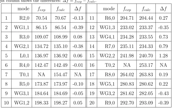
Table 1: Measured and calculated eigenfrequencies in MHz, corresponding to the mode shapes of Figure 3. The right column shows the differences: ∆f = fexp− fcalc.
mode fexp fcalc ∆f mode fexp fcalc ∆f
1 R2,0 70.54 70.67 -0.13 11 R6,0 204.71 204.44 0.27 2 WG1,1 86.15 86.54 -0.39 12 WG1,3 233.02 233.37 -0.35 3 R3,0 109.07 108.99 0.08 13 WG4,1 234.28 233.55 0.73 4 WG2,1 134.72 135.10 -0.38 14 R7,0 235.11 234.33 0.79 5 L0,1 136.97 136.92 0.06 15 WG2,2 241.98 240.70 1.28 6 R4,0 142.47 142.49 -0.01 16 T0,2 NA 253.17 NA 7 T0,1 NA 154.47 NA 17 R8,0 264.02 263.83 0.19 8 R5,0 173.87 173.97 -0.10 18 WG5,1 280.83 280.62 0.22 9 WG3,1 184.64 184.69 -0.05 19 WG3,2 281.62 282.05 -0.43 10 WG1,2 198.33 198.27 0.05 20 R9,0 292.70 293.09 -0.39
In order to evaluate the measurement uncertainty for the Young modulus and the Poisson
261
ratio, due to the measurement uncertainty of the fiber diameter, we supposed that the fiber
diameter is now 32.8µm. The best evaluation of the parameters is E = 70.0 GPa and
263
ν = 0.350 with σres= 0.17 MHz. Therefore, an error in the evaluation of the fiber diameter
264
of 0.1µm propagates an error of 0.4 GPa in the Young modulus. But it is remarkable that
265
the Poisson ratio is not sensitive to the diameter uncertainty. The evaluation of the Young
266
modulus is also sensitive to the density, with a sensitivity ∂E/∂ρ = 0.026 GPa/(kg/m3).
267
If the uncertainty of the fiber density is neglected, the result is E = (69.6 ± 0.4) GPa and
268
ν = 0.350 ± 0.001.
269
The Young modulus and the Poisson ratio were determined by considering only 9
exper-270
imental frequencies below 210 MHz. We must verify now if determined parameters give the
271
correct prediction of the other eigenfrequencies. Table 1 shows the comparison between the
272
experimental and calculated frequencies up to 300 MHz with the parameters d = 32.7µm,
273
E = 69.6 GPa, ν = 0.350 and ρ = 2700 kg/m3. Each experimental frequency fexp is an
274
average of several measured eigenfrequencies. The relative errors ∆ = (fexp − fcalc)/fcalc
275
remain under 0.5% for all the calculated frequencies below 300 MHz. The W G(2, 1) mode
276
is located before the ”breathing” L(0, 1) mode, in agreement with our initial guess.
277
Moreover, the correlation between the calculated and the experimental frequencies is
278
quite good for 31 modes up to the frequency of the Rayleigh mode R(15, 0), which is
calcu-279
lated at 466 MHz and measured at 464 MHz. The relative residuals ∆ = (fexp− fcalc)/fcalc
280
are plotted in Fig. 4. For all the measured eigenfrequencies the relative error is below 0.5%.
281
3.5. The limits of the 2-dimensional approach
282
Though the 2D model is capable to fit rather well most of the measured
eigenfrequen-283
cies, it cannot explain some particular features observed in the experimental spectrum, in
284
particular the unexpected weakness of the ”breathing mode” line at 137 MHz.
285
In the 2D approach, the propagation of acoustic waves along the fiber axis is neglected.
286
We implicitly assume that the group velocities of the excited guided modes are zero. In
287
order to evaluate an upper limit for the group velocity, we must take into account of the
288
finite length of the pump line, which determines a cutoff in the wave vector spectrum of
289
the excited guided modes. The cutoff wave number is roughly 1/Lp = 1/0.1 = 10 mm−1,
where Lp is the length of the pump spot. The propagation of guided modes can be ignored
291
during the acquisition time Ta = 2µs only if their group velocity is much lower than vgmax=
292
Lp/Ta = 50 m s−1. In consequence, the 2D approach is valid only if the group velocity is
293
inferior to 50 m s−1 for all wave vectors k . 2π · 10 mm−1.
294
The group velocity is zero for pure cross-section modes, i.e. with the k = 0 guided
295
modes. But for some modes, the variation of the group velocity with k may be too rapid
296
between the zero and the cutoff wave vector kmax = 2π · 10 mm−1 and this would result in a
297
quick vanishing signal and thus a strong apparent damping of the measured vibrations. In
298
the spectral domain, this will result in weak and broad spectral line.
299
The fact that most of the spectral lines displayed in Fig. 2 have relatively high amplitudes
300
proves a posteriori that the group velocities of most guided modes are not much larger than
301
the above estimated value 50 m s−1. However, the condition vg < 50 m s−1 may not be
302
fulfilled for some modes, in particular for the breathing mode.
303
The 2D model does not take into account the possible Zero Group Velocity modes (ZGV)
304
that may be excited in a cylinder. Such modes are known in structures capable of guiding
305
acoustic waves, such as plates [29]. The existence of ZGV modes in a cylinder is predicted
306
theoretically [30]. The ZGV modes can exhibit very high quality factors in the range of
307
Q = 1000 − 10000. Moreover, it is known that ZGV eigenfrequencies are different from
308
the cross-section eigenfrequencies. The differences between cross-section and ZGV
eigen-309
frequencies could explain some discrepancies between the experimental and the calculated
310
eigenfrequencies in the 2D modeling.
311
4. Conclusion
312
This paper presents a method to evaluate the transverse Young modulus and Poisson
313
ratio of a micrometric metallic wire by using laser resonant ultrasound spectroscopy. A
314
precision of 0.7% for the Young modulus and 0.3% for the Poisson ratio of an aluminum
315
fiber was achieved.
316
The pump laser was shaped as a line spot parallel to the fiber axis in order to excite
317
cross section eigenmodes. Using a stabilized homodyne Michelson interferometer, the cross
section eigenfrequencies were measured up to 500 MHz. The 2D vibration model of the wire
319
proved to be in good agreement for about 30 measured eigenfrequencies within an accuracy
320
of 0.5% in the 50-500 MHz range.
321
Nevertheless, the spectral resolution can be improved by increasing the acquisition time
322
windows, as some modes are not completely damped 2µs after the excitation. The improved
323
resolution could be useful to detect minute geometrical defects of the cylinder through the
324
observation of the degeneracy lifting of some modes. Furthermore, the measurement of high
325
frequency Rayleigh modes could be useful to probe the mechanical properties of the material
326
in the vicinity of the surface, as the displacements of high frequency Rayleigh modes are
327
localized mainly near the surface.
328
In order to achieve ultimate precision for the evaluation of the elastic parameters of
329
fibers, it is essential to take into account the propagation of guided modes along the fiber
330
and therefore to carry out the 3-dimensional modeling of the mechanical system and then to
331
determine the eigenfrequencies of the Zero Group Velocity modes (ZGV). Such modes could
332
be useful to improve the precision in the determination of the elastic parameters and could
333
give access to the determination of the intrinsic damping of the material, i.e. the imaginary
334
part of the Young modulus.
335
The application of the LRUS method is not restricted to metallic fibers. We intend to
336
apply more extensively our LRUS method to characterize fibers used in reinforced composite
337
materials, such as carbon, glass, kevlar and vegetal fibers. The study of vegetal fibers, in
338
particular flax fiber, which is a hollow structure approximately cylindrical, requires the
339
association of LRUS with a method to determine the actual geometry of the fiber, such as
340
digital holographic tomography.
341
References
342
[1] R. G. Leisure, F. A. Willis, Journal of Physics: Condensed Matter 9 (1997) 6001.
343
[2] W. M. Visscher, A. Migliori, T. M. Bell, R. A. Reinert 90 (1991) 2154–2162.
344
[3] A. Migliori, J. D. Maynard, Review of Scientific Instruments 76 (2005) 121301.
[4] B. J. Zadler, J. H. L. Le Rousseau, J. A. Scales, M. L. Smith, Geophysical Journal International 156
346
(2004) 154–169.
347
[5] A. Yoneda, Y. Aizawa, M. M. Rahman, S. Sakai, Japanese Journal of Applied Physics 46 (2007) 7898–
348
7903.
349
[6] A. Yaoita, T. Adachi, A. Yamaji, NDT&E International 38 (2005) 554–560.
350
[7] P. Sedl´ak, M. Landa, H. Seiner, L. Bicanov´a, L. Heller, in: 1st International Symposium on Laser
351
Ultrasonics: Science, Technology and Applications, July-16-18, Montr´eal, Canada.
352
[8] S.-K. Park, S.-H. Baik, H.-K. Cha, S. J. Reese, D. H. Hurley, J. Korean Phys. Soc. 57 (2010) 375–379.
353
[9] S. Sato, K. Inagaki, V. E. Gusev, O. B. Wright, AIP Conference Proceedings 463 (1999) 424–426.
354
[10] D. H. Hurley, S. J. Reese, F. Farzbod, Journal of Applied Physics 111 (2012) 053527.
355
[11] N. Nakamura, H. Ogi, M. Hirao, Acta Materialia 52 (2004) 765 – 771.
356
[12] A. Amziane, M. Amari, D. Mounier, J.-M. Breteau, N. Joly, J. Banchet, D. Tisseur, V. Gusev,
Ultra-357
sonics 52 (2012) 39–46.
358
[13] A. Amziane, M. Amari, D. Mounier, J.-M. Breteau, N. Joly, M. Edely, M. Larcher, P. Noir´e, J. Banchet,
359
D. Tisseur, V. Gusev, Proc. of SPIE 8082 (2011) 808224.1–808224.10.
360
[14] S. Petit, M. Duquennoy, M. Ouaftouh, F. Deneuville, M. Ourak, S. Desvaux, Ultrasonics 43 (2005)
361
802–810.
362
[15] F. Deneuville, M. Duquennoy, M. Ouaftouh, M. Ourak, F. Jenot, S. Desvaux, Ultrasonics 49 (2009)
363
89–93.
364
[16] R. E. Smith, J. Appl. Phys. 43 (1972) 2555–2561.
365
[17] D. S´egur, Y. Guillet, B. Audoin, Journal of Physics: Conference Series 278 (2011) 012020.
366
[18] C. Baley, Composites Part A: Applied Science and Manufacturing 33 (2002) 939 – 948.
367
[19] C. Sauder, J. Lamon, R. Pailler, Carbon 42 (2004) 715–725.
368
[20] C. B. Scruby, L. E. Drain, Laser ultrasonics: techniques and applications, 1990.
369
[21] Heraeus, 2012. AlSi 1%, The Aluminum Fine Wire Solution.
370
[22] M. Silk, K. Bainton, Ultrasonics 17 (1979) 11 – 19.
371
[23] I. Viktorov, Rayleigh and Lamb waves, 1967.
372
[24] D. Clorennec, D. Royer, H. Walaszek, Ultrasonics 40 (2002) 783?789.
373
[25] H. Ogi, K. Sato, T. Asada, M. Hirao, J. Acoust. Soc. Am. 112 (2002) 2553–2557.
374
[26] P. Picart, J. Leval, D. Mounier, S. Gougeon, Appl. Opt. 44 (2005) 337–343.
375
[27] J. Leval, P. Picart, J. P. Boileau, J. C. Pascal, Appl. Opt. 44 (2005) 5763–5772.
376
[28] Nist/sematech e-handbook of statistical methods, 2012. Response surface designs.
377
[29] C. Prada, D. Clorennec, D. Royer, The Journal of the Acoustical Society of America 124 (2008) 203–212.
378
[30] C. Prada-Julia, 2012. Institut Langevin, ESPCI, Paris, confirmed theoretically the existence of ZGV
modes in cylinders (personal communication).
Figure 3: Mode shapes of the first 20 calculated eigenmodes of an aluminum cylinder. Numbers correspond to the ordering numbers of Table 1. Category of each eigenmode: Rayleigh (R), Wave Gallery (WG), longitudinal (L) or torsional (T) is indicated. Rayleigh modes are characterized by predominant radial components. Colors represent the magnitude of the displacements: the deep blue color means a zero displacement, i.e. the nodal areas of the mode shape and the red color is for the maximum magnitude. The arrows indicate both the direction and the magnitude of displacements.
Figure 4: Percentage of relative error between experimental and calculated eigenfrequencies with the pa-rameters: d = 32.7µm, E = 69.6 GPa, ν = 0.350 and ρ = 2700 kg/m3.