Applications of machine learning : consumer credit risk analysis

Applications of Machine Learning: Consumer

Credit Risk Analysis

by

Danny Yuan

B.S. Electrical Engineering and Computer Science and B.S.

Mathematics, Massachusetts Institute of Technology (2013)

Submitted to the Department of Electrical Engineering and Computer

Science

in partial fulfillment of the requirements for the degree of

Master of Engineering in Electrical Engineering and Computer Science

at the

MASSACHUSETTS INSTITUTE OF TECHNOLOGY

June 2015

Copyright

© 2015 Massachusetts Institute of Technology, All rights

reserved.

The author hereby grants to M.I.T. permission to reproduce and to distribute publicly paper and electronic copies of this thesis document in whole and in part in any medium now known or

hereafter created.

Author . . . .

Department of Electrical Engineering and Computer Science

May 14, 2015

Certified by . . . .

Andrew W. Lo

Charles E. and Susan T. Harris Professor; Professor of Electrical

Engineering and Computer Science; Professor of Sloan School of

Management

Thesis Supervisor

Certified by . . . .

John Guttag

Professor of Electrical Engineering and Computer Science

Thesis Supervisor

Accepted by . . . .

Professor Albert R. Meyer

Chairman, Master of Engineering Thesis Committee

Applications of Machine Learning: Consumer Credit Risk

Analysis

by

Danny Yuan

Submitted to the Department of Electrical Engineering and Computer Science on May 14, 2015, in partial fulfillment of the

requirements for the degree of

Master of Engineering in Electrical Engineering and Computer Science

Abstract

Current credit bureau analytics, such as credit scores, are based on slowly varying consumer characteristics, and thus, they are not adaptable to changes in customers behaviors and market conditions over time. In this paper, we would like to ap-ply machine-learning techniques to construct forecasting models of consumer credit risk. By aggregating credit accounts, credit bureau, and customer data given to us from a major commercial bank (which we will call the Bank, as per confidentiality agreement), we expect to be able to construct out-of-sample forecasts. The result-ing models would be able to tackle common challenges faced by chief risk officers and policymakers, such as deciding when and how much to cut individuals account credit lines, evaluating the credit score for current and prospective customers, and forecasting aggregate consumer credit defaults and delinquencies for the purpose of enterprise-wide and macroprudential risk management.

Thesis Supervisor: Andrew W. Lo

Title: Charles E. and Susan T. Harris Professor; Professor of Electrical Engineering and Computer Science; Professor of Sloan School of Management

Thesis Supervisor: John Guttag

Acknowledgements

Over the years I have been very fortunate to attend MIT and have the pleasure to work with a few great people. I would like to express my sincere gratitude to the following people.

First and foremost, I want to give a big thanks to BigData@CSail for providing funding for this research project and providing me with a research assistantship. My education would not have been complete and this paper would not have been possible without their generous support.

Next, I would like to thank my supervisors, Andrew Lo and John Guttag, for giv-ing me such an engaggiv-ing and interestgiv-ing topic to work with. This project has beautiful elements from both artificial intelligence, the field of concentration for my Masters degree, and in finance, my career interest. My supervisors are more knowledgeable in their respective areas of expertise than anyone I know. I was given insights into the mixture of the two fields that I would not have gotten elsewhere.

I would also like to thank David Fagnan, a graduate student who has been su-pervising me on this project, for his patience and his sharing of his vast knowledge in the field of consumer credit risk. There were many hurdles over the course of the paper, without his advice and words of encouragement, the project would not have been possible.

Finally, I would like to thank my parents and my sister for their sacrifices made along the way to ensure the greatest education I can ever have. At times, I have certainly been so absorbed with academics and work that I neglected other parts of my life. Thank you for always being there for me.

Contents

1 Introduction to Consumer Credit Risk Modeling 11

1.1 Introduction . . . 11

1.2 Credit Scoring . . . 12

1.3 Defining the Prediction Problem based on Datasets . . . 13

1.4 Outline of this Paper . . . 15

2 Data Preparation 17 2.1 Data Cleaning . . . 17

2.2 Splitting into Training and Testing sets . . . 18

3 Feature Selection 21 3.1 Methods for Selection . . . 21

3.1.1 Selection via Random Forest . . . 22

3.1.2 Selection via Logistic Regression . . . 26

3.2 The List of Selected Features . . . 26

4 Using Machine Learning Algorithms for Credit Scoring 29

4.1 Logistic Regression . . . 29

4.1.1 Building the Model . . . 30

4.1.2 Interpreting the Model . . . 33

4.2 Support Vector Machines . . . 34

4.2.1 Building the Model . . . 36

4.2.2 Evaluating the Model . . . 38

4.3 Random Forest . . . 40

4.3.1 Decision Trees . . . 40

4.3.2 Building Random Forest Models . . . 45

4.3.3 Evaluating the Model . . . 50

5 Closing Remarks 53 5.1 Conclusion . . . 53

5.2 Further Work . . . 54

Bibliography 55

List of Figures

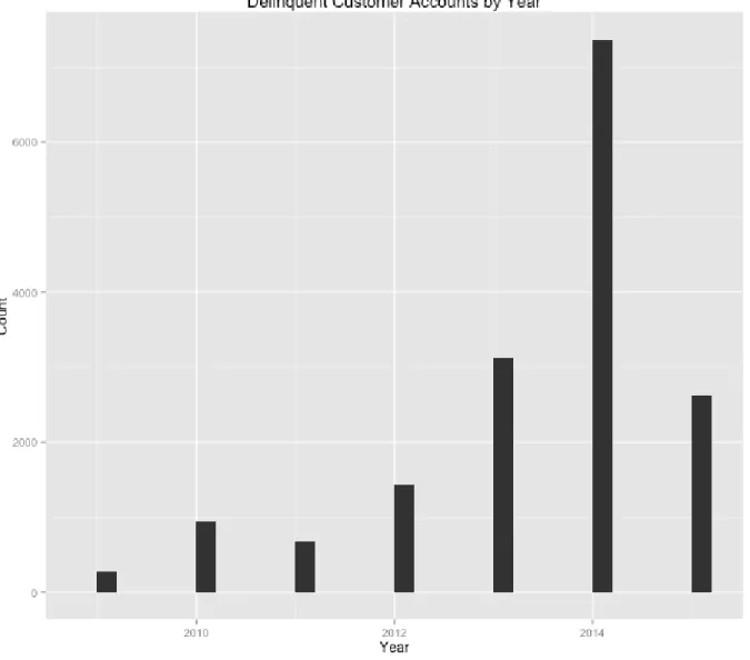
1-1 Distribution of the year which delinquent customers become delinquent 14

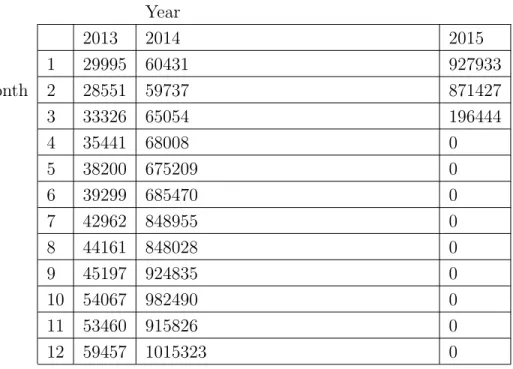
1-2 Distribution of Statements data by year and month, given to us by the

Bank, as of March 2015 . . . 15

2-1 The datasets and its most relevant features . . . 20

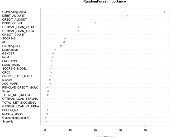
3-1 Importance values returned by Random Forest . . . 23

3-2 Graph of importance values returned by Random Forest . . . 24

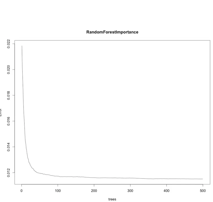
3-3 Error rate as the number of trees increase . . . 25

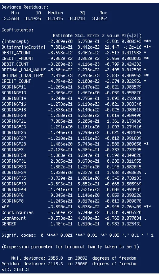
3-4 The model summary returned by R . . . 27

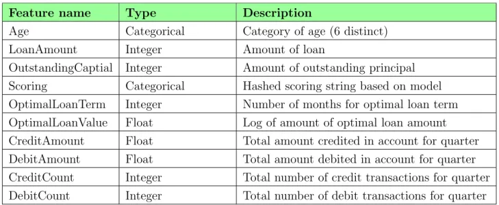
3-5 Description of selected features . . . 28

4-1 The training set’s distribution of scores returned by logistic regression by positive (delinquent, Dt = 1) and negative (non-delinquent, Dt = 0) examples . . . 31

4-2 Enrichment and recall returned by logistic regression as a function of threshold for the training set . . . 32

4-3 Confusion matrix of the resulting classifier on the test set at threhold 0.02 . . . 32

4-4 Evaluation of our model . . . 32

4-5 The model coefficients . . . 33

4-6 ROC curves for logistic regression. Training set is represented in red and testing set is represented in green. . . 35

4-7 A table showing the number of support vectors for different values of soft penalty error and class weights . . . 36

4-8 A table showing the rate of training error for different values of soft penalty error and class weights . . . 37

4-9 A table showing the rate of cross validation error for different values of soft penalty error and class weights . . . 37

4-10 A table showing computed precision value for different values of soft penalty error and class weights . . . 39

4-11 A table showing computed recall value for different values of soft penalty error and class weights . . . 39

4-12 A decision tree to classify delinquent customer accounts by the variable OutstandingCapital . . . 41

4-13 Accuracy and run time data for CART algorithms as a function of density and tree size . . . 42

4-14 Relative error for different tree sizes for density = 0.0001 . . . 43

4-15 ROC curve on testing data for densities shown in Figure 4-13. The red line corresponds to density = 0.01 and the green curve corresponds to density = 0.001. The other densities overlap each other. . . 44

4-16 ROC curve on training data for various values of number of trees: 1 (black), 10 (red), 100 (green), and 1000 (blue) . . . 46

4-17 ROC curve on testing data for various values of number of trees: 1 (black), 10 (red), 100 (green), and 1000 (blue) . . . 47

4-18 ROC curve on training data for various values of minimum node size: 1 (black), 10 (red), 100 (green), and 1000 (blue) . . . 48

4-19 ROC curve on testing data for various values of minimum node size: 1 (black), 10 (red), 100 (green), and 1000 (blue) . . . 49

4-20 AUC values on testing sets for different values of number of trees and minimum node size . . . 50

4-21 AUC values on training sets for different values of number of trees and minimum node size . . . 50

Chapter 1

Introduction to Consumer Credit

Risk Modeling

This chapter gives an overview of the consumer credit risk markets and why it is an important topic to study for purposes of risk management. We introduce the data we used for this paper and the prediction problem we are trying to solve. Finally we describe how we reformatted the data and how we split the data into training and testing sets.

1.1

Introduction

One of the most important considerations in understanding macroprudential and systemic risk is delinquency and defaults of consumer credit. In 2013, consumer spending encompassed approximately 69 percent of U.S. gross domestic product. Of the $3.098 trillion of outstanding consumer credit in the United States in the last quarter of 2013, revolving credit accounts for over 25 percent of it ($857.6 billion). A 1% increase in accuracy of identifying high-risk loans could prevent losses for over$8 billion. Because of the risks inherent in such a large portion of our economy, building models for consumer spending behaviors in order to limit risk exposures in this sector is becoming more important.

12 CHAPTER 1. INTRODUCTION TO CONSUMER CREDIT RISK MODELING

the lending institutions and credit bureaus. Credit bureaus collect consumer credit data in order to compute a score to evaluate the creditworthiness of the customer; however, these metrics do not adapt quickly to changes in consumer behaviors and market conditions over time. [KKL10] We propose to use machine-learning techniques to analyze datasets provided to us by a major commercial bank (which we shall refer to as the ‘’Bank” as per our confidentiality agreements). Since consumer credit models are relatively new in the space of machine learning, we plan to compare the accuracy and performance of a few techniques. There are many ways to do feature selections, splitting of data into training and testing sets, regularization of parameters in algorithms to handle overfitting and underfitting, and various kernel functions to handle higher order non-linearity in the features. We will explore many of these.

By aggregating proprietary data sets from the Bank, we will train and optimize different models in order to predict if a customer will be delinquent in their payments for the next quarter. We will then test the models with out of sample data.

1.2

Credit Scoring

The goal of credit scoring is to help financial institutions decide whether or not to lend to a customer. The resulting test is usually a threshold value that helps the decision maker make the lending decision. Someone above the threshold is usually considered a credit worthy customer who is likely to repay the financial obligation. Someone below the threshold is more at risk, and less likely to repay the financial obligation. Such tests can have a huge impact on profitability for banks; a small fraction of a percentage improvement will have tremendous impact. [Ken13]

There are two types of credit scoring, application scoring and behavioral scoring. Application scoring is done at the time for application and estimates the probability of default over some periods. Behavioral scoring is used after credit has been granted, and generally is used to monitor an individual’s probability of default over some periods. This paper focuses on the latter of the two; in particular, we will try to monitor the Banks’ customers and create metrics to flag customers that have become

1.3. DEFINING THE PREDICTION PROBLEM BASED ON DATASETS 13

risky over time. [Ken13] Given these new metrics, the Bank could take actions against flagged customers, such as closing their accounts or suspending further loans.

1.3

Defining the Prediction Problem based on Datasets

We were given 5 datasets by the Bank. We shall call these data sets: Accounts, Banks, Customer, Records, and Statements. Respectively, they contain roughly 270,000 ob-servations of 130 variables, 84,000 obob-servations of 230 variables, 85,000 obob-servations of 20 variables, 53,000 observations of 30 variables, and 8,900,000 observations of 40 variables. Accounts contains data on the state of the bank accounts, Bank contains data provided by the credit bureau from all banks about customers‘ loans, Customers contains a set of data about the customers, Records contains data collected at the time of loan application, and Statements contain information about credit card trans-actions, but only from 2013.

The field we are interested in is a boolean variable in the Accounts data set for whether the customer account is delinquent or not. In Figure 1-1, we can see the distribution of the year on which the delinquent customers become delinquent on their payment. We have the most delinquencies data in 2013, 2014 and the first quarter of 2015. Further looking into the Statements data in Figure 1-2, we see that the amount of Statements data jumped almost 10-fold from April 2014 to May 2014. This makes us think that the data itself is inconsistent, because of the sharp increase in the number of transactions between these two months. One possible explanation for this inconsistency could be a change in definition in what a transaction is. We decided to throw away the data after March 2014 and do predictions for each quarter of data we do keep.

The prediction problem we are trying to answer is:

Given the credit card transactions (Statements) data in the previous quarter, ag-gregated with data from Accounts, Banks, Customers, and Records data, will the customer account be delinquent in payment for the next quarter?

14 CHAPTER 1. INTRODUCTION TO CONSUMER CREDIT RISK MODELING

1.4. OUTLINE OF THIS PAPER 15

Distribution of Statements Data Year 2013 2014 2015 1 29995 60431 927933 Month 2 28551 59737 871427 3 33326 65054 196444 4 35441 68008 0 5 38200 675209 0 6 39299 685470 0 7 42962 848955 0 8 44161 848028 0 9 45197 924835 0 10 54067 982490 0 11 53460 915826 0 12 59457 1015323 0

Figure 1-2: Distribution of Statements data by year and month, given to us by the Bank, as of March 2015

In order to answer this question, we have to prepare our data so that we could run machine-learning algorithms. Since we are trying to do prediction on the next quarter based on transactions from the previous quarter, we have to first split the data sets into quarters and then merge Statements data from one quarter with Accounts data from the next quarter.

1.4

Outline of this Paper

The following is the outline of this paper:

• Chapter 2 This chapter describes how we prepared the data to be used for ma-chine learning. We will discuss how we dealt with missing values and how we divided the data into training and testing sets.

• Chapter 3 This chapter talks about how we chose to select the most significant features to be used for machine learning. We will explore two techniques used

16 CHAPTER 1. INTRODUCTION TO CONSUMER CREDIT RISK MODELING

to do this, logistic regression and random forest.

• Chapter 4 This chapter goes over the three machine learning techniques used to explore our prediction problem. We will discuss the results and interpret the findings returned by logistic regression, support vector machines, and random forest.

• Chapter 5 This chapter concludes our findings and discusses what can be done next as the next steps in building better consumer credit risk models.

Chapter 2

Data Preparation

In this chapter, we talk about what we did to clean the data into a useable format and how we defined our training and testing sets. We identify some issues we discovered with the data and how we treat missing values. We also talk about how we manipulate the data to answer our prediction problem.

2.1

Data Cleaning

In order to answer our prediction question using machine learning, we need to ma-nipulate the data to fit the input format for the algorithms. To do so, we cleaned each of the datasets before merging them together. Many of the fields in the data sets were missing, and we handled them in a special manner. For discrete variables, we replaced the field with a value of 0 and created a new column called FIELD NA, a binary dummy variable (0 or 1) to indicate whether the original field was missing. For continuous values, we replaced the missing value with the average of available data and added a binary dummy variable to indicate that it is missing.

In the accounts data set, there are about two dozens different account/product types (since much of the data are hashed to protect the confidentiality of the customer, we don‘t actually know what these types mean). Since we only have statements data from 2013 and want to use it to do prediction, we remove all delinquencies before 2013. After removing all these accounts and accounts that are closed, we were left

18 CHAPTER 2. DATA PREPARATION

with about 99,000 workable accounts and roughly 34,000 unique customers. We also generated new fields such as RemainingPayments (amount left to pay), Delinquen-cyCounts (number of times delinquent in data sets), and QuarterDelinquent (the quarter in which it was delinquent on its payment).

The customers data set was pretty straightforward. We kept the columns that are meaningful, for example, age, marital status, gender, occupation, education, credit card marker, mortgage marker, loan marker and revolving credit marker. Columns we dropped include minimum subsistence, installment loan marker, and postal code. The reason we dropped them was either the Bank told us that they are irrelevant or the data itself is mostly meaningless or un-interpretable.

In the banks dataset, there are many repeated rows, empty columns, and a lot of NA cells. The most useful data we extracted from this dataset are the number of inquiries (a row is generated whenever an inquiry is made) and the credit score for the customers. Although we had no credit scores for some of the customers, we were able to handle such observations in the manner described earlier.

For the records dataset, we are missing data on some customers, so we handled it as described earlier. After cleaning the data, we aggregated all the data by merging them by their customer id field.

Finally in the statements data, we aggregated the total amount debited and cred-ited in each quarter, and we created new columns, CreditCount and DebitCount, which represent the number of credit and debit transactions.

2.2

Splitting into Training and Testing sets

Since we are trying to build a prediction model for delinquency rates, we first need data to build the model. We also need data to test whether our model makes correct predictions on new data. The first set of data is called the training set, the latter set of data is called the testing set, also known as hold-out set. The training set is the data that we feed into the machine-learning model (logistic regression, support vector machines, random forest.etc). The test set is the set of data we feed into our

2.2. SPLITTING INTO TRAINING AND TESTING SETS 19

trained model to check the accuracy of our models.

Since we are trying to predict delinquency for the next quarter based on statements data in the previous quarter, we split the statements data into quarters. January, February and March will be considered quarter 1, April, May and June will be con-sidered quarter 2, and so on. We then merged the data in such a way that we have customer data for quarter 2 and statements data for quarter 1 in 1 row. After this, we create training and testing sets by creating a new column with random values between 0 and 1, and pick a threshold. We picked 0.7 because we want there to be roughly 70% of our data in the training set and the rest in the testing set. We are also careful about making sure all customers are either in the training set or testing set. After we moved all the customer accounts chosen in the testing set into the training set, we ended up with roughly 80% of our data in the training and 20% of our data in the testing set.

Cleaning the data was probably the most time-consuming part of the project, because there were a lot of questions we needed to answer before it could be done. Figuring out what the prediction problem is given the limited amount of data we have, understanding what each of the fields mean through translation of the variables, and communicating with our client took up most of one semester. However, once that was out of the way, we were ready to move onto the next phrase of the project, feature selection.

20 CHAPTER 2. DATA PREPARATION

Chapter 3

Feature Selection

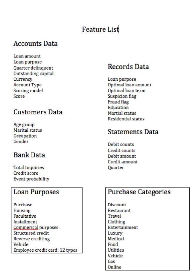
In this chapter, we explore ways to find features to use for training our machine learning models. We have shown the features provided to us in the data set by the Bank in Figure 2-1. However, many of the features contribute little to no help in predicting whether the customer account will eventually go delinquent. As such, it is important to find the features that are relevant in order to bring down the run time of the algorithms and give us a better understanding of which features are actually meaningful.

3.1

Methods for Selection

We present two widely used methods in selecting features of significance in the ma-chine learning literature. The methods come from supervised learning, the task of inferring a function from previously labeled examples. It uses training data to infer a function, which could be used to map values for data in the testing set. Logistic regression is commonly used to do prediction on bankruptcy. [FS14] Random forest also provides importance values to input features. We will use these two methods to do feature selection.

22 CHAPTER 3. FEATURE SELECTION

3.1.1

Selection via Random Forest

Random forest is an ensemble learning method for classification that trains a model by creating a multitude of decision trees and outputting the mode of the classes re-turned by the individual trees. The algorithm applies the technique of bootstrapping aggregation, also known as bagging, to tree learners. Given a training set X = x1, , xn

and output Y = y1, , yn, bagging repeatedly selects a sample at random with

replace-ment from the training set and fits trees to the samples: For b = 1, ..., B:

1. Sample, with replacement n training examples from Xb, Yb

2. Train a decision tree fb on the samples.

After training, predictions for unseen examples are made by averaging the predic-tions or taking the mode in the case of decision trees.

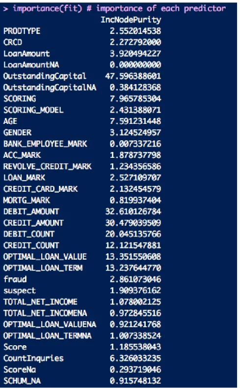
Random forest follows the general scheme of bagging but differs by using a mod-ified tree-learning algorithm that selects, at each iteration of the learning process, a random subset of features. We use random forest to do feature selection because of its ability to rank the importance of the variables. To measure the importance of the variables, we first fitted a random forest to the data. During this step, the classification error rate for each data point is recorded and averaged over the forest. To measure the importance of a variable, each predictor variable is then permuted and the error rate is recomputed. The importance score of a variable is computed by first averaging the differences in error rate before and after the permutation of the predictor variables, and then dividing the result by the standard deviation of the differences. The list of importance values can be seen in Figure 3-1. In Figure 3-2, we plotted the importance values of the variables. The most important features appear to be OutstandingCapital, DebitAmount, and CreditAmount. In Figure 3-3, we have plotted the error rate of random forest as we increase the number of trees/samples. As expected, the error decreases as we increase the number of trees/samples in our bootstrapping procedure.

3.1. METHODS FOR SELECTION 23

24 CHAPTER 3. FEATURE SELECTION

3.1. METHODS FOR SELECTION 25

26 CHAPTER 3. FEATURE SELECTION

3.1.2

Selection via Logistic Regression

Logistic regression is one of the most important generalized linear models. It is most often used to predict the probability that an instance is part of a class. In our case, we want to use logistic regression with lasso regularization to predict the probability that a customer account will default in the next quarter by predicting values that are restricted to the (0,1) interval. It does so by modeling the probability in terms of numeric and categorical inputs by assigning coefficients. By running the summary() command in R, we are able to see which coefficient values are statistically significant. Looking at Figure 3-4, we see that OustandingCapital, Age, CreditAmount, Deb-itAmount, OptimalLoanValue, OptimalLoanTerm, LoanAmount and CreditCount are some of the significant features. Two of the Scoring category dummy variables were also significant. Interestingly, these were all in the top 10 features returned by Random Forest. The only one which logistic regression did not include is DebitCount.

3.2

The List of Selected Features

Combining the results returned by random forest and logistic regression, we have decided to take all the significant features, including DebitCount, into our training models. A brief description of the selected features is listed in Figure 3-5.

Since we are doing predictions based on statements data from the previous quarter to predict delinquency in the next quarter, it is reassuring to see that CreditAmount, DebitAmount, CreditCount, and DebitCount are significant features for our predic-tion problem. These features were generated by aggregating the data in the state-ments dataset. Furthermore, LoanAmount, OutstandingCapital, OptimalLoanTerm, and OptimalLoanValue were features related to the loan itself, so it is reasonable that they are included in the selected features. Finally, Age and Scoring were also included as well: studies have shown that Age is correlated to income and scoring is based on the creditworthiness of the customer.

3.2. THE LIST OF SELECTED FEATURES 27

28 CHAPTER 3. FEATURE SELECTION

Selected Features

Feature name Type Description

Age Categorical Category of age (6 distinct) LoanAmount Integer Amount of loan

OutstandingCaptial Integer Amount of outstanding principal Scoring Categorical Hashed scoring string based on model OptimalLoanTerm Integer Number of months for optimal loan term OptimalLoanValue Float Log of amount of optimal loan amount CreditAmount Float Total amount credited in account for quarter DebitAmount Float Total amount debited in account for quarter CreditCount Integer Total number of credit transactions for quarter DebitCount Integer Total number of debit transactions for quarter

Chapter 4

Using Machine Learning

Algorithms for Credit Scoring

This chapter explores the results of three machine learning algorithms: logistic regres-sion, support vector machines, and random forest. These methods are chosen because of their suitability as solutions to the low-default portfolio problem. In this chapter, we look at the accuracy of these models by fine-tuning the threshold values on classi-fier inputs. The comparative assessment of these classification methods is subjective and will influenced by the Bank’s preferences to precision and recall values. As such, we present a range of values and allow the reader to assess the tradeoffs.

4.1

Logistic Regression

For our classification problem of finding delinquent customers, logistic regression is the classic model for binary classifications. It is usually the go-to for users and offers a baseline for other machine learning algorithms. Logistic regression doesn’t perform well with a large number of features or categorical features with a large number of values, but it still predicts well when working with correlated features.

30 CHAPTER 4. USING MACHINE LEARNING ALGORITHMS FOR CREDIT SCORING

4.1.1

Building the Model

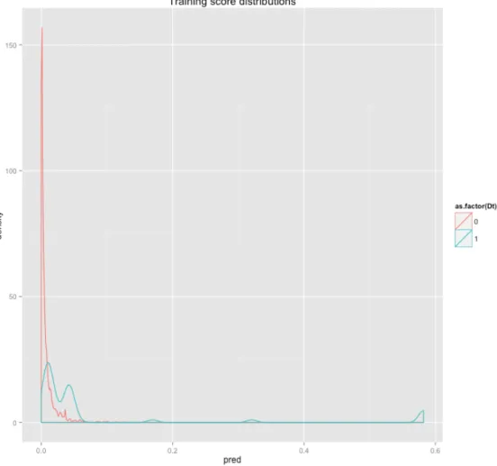
In Figure 4-1, we see the distributions of the scores returned by logistic regression for the delinquent and non-delinquent examples. The distribution of non-delinquent customers is more heavily weighted towards 0 than that of the delinquent customers. Our goal is to use the model to classify examples in our testing set. Therefore, we should assign high scores to delinquent customers (Dt = 1) and low scores to non-delinquent customers (Dt = 0). Both distributions seem to be concentrated towards 0, meaning the scores for both instances seem to be low. The distribution for the non-delinquent customers decays to 0 faster than that of the delinquent customers. From this, we can see the model subpopulations where the probability of delinquency is higher.

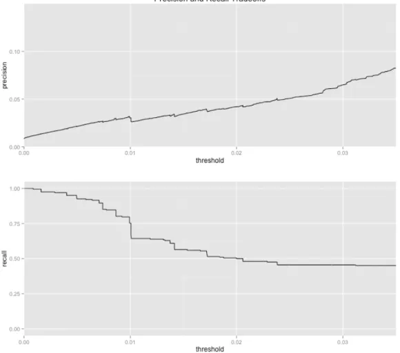
For logistic regression to solve our classification problem, we have to choose a threshold for the examples to be positive and negative. When picking a threshold, we have to consider the tradeoffs between precision and recall. Precision is the fraction of predicted positive examples that are actually positive. Recall is the number of actual positive examples our model can find. From looking at Figure 4-2, we see that a high threshold would make more precise classifications but identify fewer cases while a low threshold would identify more cases at the cost of identifying false positives. The user should consider his preference to precision and recall when making this tradeoff. For us, choosing a threshold in the neighborhood of 0.02 seems best, since we will have a roughly 50 % recall while maintaining a high precision.

We evaluated our model on the test set and the results are shown in Figure 4-3. Our model turns out to be a low precision classifier with a precision of 0.1020408 but it was able to find 55.56% of the delinquent examples in the test set, at a rate 9.852608 times higher than the overall average. Next, we will see how well the model fits our data, and what we can learn from the models.

4.1. LOGISTIC REGRESSION 31

Figure 4-1: The training set’s distribution of scores returned by logistic regression by positive (delinquent, Dt = 1) and negative (non-delinquent, Dt = 0) examples

32 CHAPTER 4. USING MACHINE LEARNING ALGORITHMS FOR CREDIT SCORING

Figure 4-2: Enrichment and recall returned by logistic regression as a function of threshold for the training set

actual

non-delinquent delinquent predicted non-delinquent 816 4

delinquent 44 5

Figure 4-3: Confusion matrix of the resulting classifier on the test set at threhold 0.02 precision 0.1020408 recall 0.555556 enrich 9.852608 p-value 2.164682e-86 pseudo R-squared 0.2047119

4.1. LOGISTIC REGRESSION 33

Figure 4-5: The model coefficients

4.1.2

Interpreting the Model

The coefficients in Figure 4-5 returned by logistic regression tell us the relationships between the input variables and the output variables. Every categorical variable is expanded into n − 1 variables where n is the number of possible values of that vari-able. Negative coefficients indicate that the variables are negatively correlated to the probability of the event, whereas positive coefficients indicate that the variables are positively correlated to the probability of the event. Furthermore, we should only consider variables that are statistically significant. As discussed in Section 3.1.2, only two of the Scoring dummy categorical variables are significant.

The coefficient for Gender is 0.148443151, so that means that the odds of a male customer being delinquent are exp(0.148443151) = 1.16 times more likely compared to the reference level (females). For a female with a probability of delinquency of 5% (with odds p/(1 − p), 0.05/0.95 = 0.0526), the odds for a male with all else character-istics equal are 0.0526 ∗ 1.16 = 0.061016, which corresponds to delinquent probability of odds/(1 + odds) = 0.061016/1.061016, which is roughly 5.74%.

For numerical variables such as CREDITCOUNT, we can similarly interpret the coefficients. The coefficient on CREDITCOUNT is -0.047937984. This means that ev-ery credit transactions lowers the odds of delinquency by exp(−0.047937984) = 0.953.

34 CHAPTER 4. USING MACHINE LEARNING ALGORITHMS FOR CREDIT SCORING

For a male customer with no transactions, the odds of going delinquent for a similar customer with 10 credit transactions would be about 0.061016 ∗ 0.95310 _{= 0.037702,}

which corresponds to delinquent probability of 3.63%.

Logistic regression models are trained by maximizing the log likelihood of the data given the training data, or minimizing the sum of the squared residual deviances. De-viance measures how well the model fits the data. We calculated the p-value to see how likely it is that the reduction in deviance was by chance. Another interpretation of the p-value is the probability of obtaining the results when the null hypothesis is true. A low p-value will give significant meaning to our results. The p-value turned out to be 2.164682e-86, which is very unlikely to occur by chance. We also computed the pseudo R-squared based on deviances to see how much of the deviance is explained by the model. The model explained 20.4% of the deviance.

We also drew the ROC curves in Figure 4-6. The ROC (receiver operating char-acteristic) curve graphs the performance of the model of various threshold values. It plots the true positive rate against the false positive rate. Notice that the curve for the testing set is rather “steppy,” because of the small fraction of delinquent customer accounts in our data set. We have also calculated the area under the curve. For the training test, it is 0.8713662. For the testing set, it is 0.7985788.

4.2

Support Vector Machines

Support vector machines use landmarks (support vectors) to increase the power of the model. It is a kernel-based classification approach where a subset of the training examples is used to represent the kernel. The kernels help lift the classification problem into a higher dimension space where the data could be as linearly separable as possible. It is useful for classifications when similar data are likely to belong to the same class and where it is hard to know the interaction or combinations of the input variables in advance. It was also found to be relevant in many financial applications recently. [ML05]

4.2. SUPPORT VECTOR MACHINES 35

Figure 4-6: ROC curves for logistic regression. Training set is represented in red and testing set is represented in green.

36 CHAPTER 4. USING MACHINE LEARNING ALGORITHMS FOR CREDIT SCORING

Support Vectors Soft margin penalty

1 10 100 1000 0.01 3607 3045 2668 2605 Class weights 0.1 3601 3057 2654 2606 1 3684 3201 2771 2668 10 6607 6071 5245 4418 100 23832 17660 11858

Figure 4-7: A table showing the number of support vectors for different values of soft penalty error and class weights

4.2.1

Building the Model

There are many kernel functions we could use but the radial basis function kernel or Gaussian kernel is probably best for our classification problem because of the unknown relationships of our input variables. The Gaussian kernel on two samples x and x0 is defined to be

K(x, x0) = exp(−kx − x

0_k2

2σ2 )

The feature space of this kernel is infinite [Mur12], since the Taylor expansion is:

K(x, x0) = exp(−kx − x 0_k2 2σ2 ) = ∞ X j=0 (xTx0)j j! exp(− 1 2kxk 2_)exp(−1 2kx 0_k2₎

There are two parameters to SVM that we can adjust to get the most accurate model. They are the soft margin penalty and the class weights. The soft margin penalty allows us to specify our preferences for not moving training examples over getting a wider margin. This depends on if we want a complex model that applies weakly to all data or a simpler model that applies strongly to a subset of data. We will explore both simple and complex models. The class weights allow us to specify the cost of getting a false positive and false negative. We will also explore various values of penalization of the two.

4.2. SUPPORT VECTOR MACHINES 37

Training Error Soft margin penalty

1 10 100 1000 0.01 0.01357 0.01166 0.0091 0.0065 Class weights 0.1 0.01358 0.01166 0.00917 0.0065 1 0.0125223 0.01109853 0.008937148 0.006644984 10 0.01845 0.01665 0.01299 0.00921 100 0.1468711 0.1193 0.07712

Figure 4-8: A table showing the rate of training error for different values of soft penalty error and class weights

Cross Validation Error Soft margin penalty

1 10 100 1000 0.01 0.01401 0.01431 0.01547 0.01827 Class weights 0.1 0.014 0.0143 0.0156 0.0183 1 0.01353436 0.01428915 0.01590162 0.01804582 10 0.02072 0.02425 0.02555 0.0272 100 0.1544 0.1253 0.0879

Figure 4-9: A table showing the rate of cross validation error for different values of soft penalty error and class weights

38 CHAPTER 4. USING MACHINE LEARNING ALGORITHMS FOR CREDIT SCORING

4.2.2

Evaluating the Model

We tested a range of values for the soft margin penalty C, namely 1, 10, 100, and 1000. We also tested a range of values for the ratio of the class weights W we assign to delinquent and non-delinquent customer accounts, namely 0.01, 0.1, 1, 10, and 100.

We have shown the values for the number of support vectors in Figure 4-7. As seen in the table, the number of support vectors increase with higher ratio assigned to the class rates of non-delinquent customers over delinquent customer accounts. The number decreases when we increase the soft margin penalty. This makes sense intuitively because a higher margin for error would lead to a wider margin and fewer support vectors.

In Figure 4-8, we show the training error for the same set of values for soft penalty error and class weights. The training error decreases as we increase the soft margin penalty. This is expected; the soft margin penalty parameter C is a regularization term use to control overfitting. As C increases, it is better to reduce the geometric margin and have more training errors. As C decreases, it is better to lower the training error and increase the geometric margin. As the ratio of non-delinquent to delinquent increases, the training error also increases. This is because the data is mostly non-delinquent. When the cost of incorrectly predicting delinquent customers goes up, there are fewer penalties in predicting non-delinquent customers, so we make more training errors.

Figure 4-9 shows the cross validation error for the testing sets. We typically want to pick C that has the lowest cross validation error. For class weight ratios of 0.01, 0.1, 1, and 10, a lower soft margin penalty (C < 1) seems to produce higher accuracy, whereas for the class weight ratio of 100, a large soft margin penalty (C > 100) would produce more accurate models.

The precision rate is shown in Figure 4-10. Precision, also known as positive predictive value, is defined as the fraction of predicted positive values that are actually positive. For class weight ratios of 0.01, 0.1, and 1, precision increases with higher

4.2. SUPPORT VECTOR MACHINES 39

Precision

Soft margin penalty

1 10 100 1000 0.01 0.0264 0.0793 0.1762 0.2159 Class weights 0.1 0.0264 0.0793 0.1762 0.2203 1 0.1013216 0.1585903 0.2026432 0.2599119 10 0.48017 0.4405 0.3789 0.3127 100 0.7533 0.6122 0.489

Figure 4-10: A table showing computed precision value for different values of soft penalty error and class weights

Recall

Soft margin penalty

1 10 100 1000 0.01 1 0.5625 0.4706 0.405 Class weights 0.1 1 0.5625 0.4819 0.4098 1 0.6052632 0.6428571 0.4893617 0.437037 10 0.39636 0.3984 0.3333 0.2639 100 0.0868 0.0825 0.0901

Figure 4-11: A table showing computed recall value for different values of soft penalty error and class weights

values of soft margin penalty C, while for class weight ratios of 10, and 100, precision decreases with higher values of soft margin penalty C. This is because of the low delinquency rates in our population. When the cost of making mistakes on delinquent customer accounts becomes high, we want to widen our geometric margin to account to capture more of the delinquent customer accounts.

Finally, we show the recall values in Figure 4-11. Recall, also known as sensitivity, is the fraction of positive examples that the model is able to identify. High sensitivity can be achieved by assigning all examples to be positive; however, such models would not be very useful. Recall is also inversely proportional to precision; therefore a high recall value usually implies a low precision value and a low recall value usually implies a high precision value. Typically, people like to aim for a precision of 0.5, but this is a tradeoff that the user himself should consider.

40 CHAPTER 4. USING MACHINE LEARNING ALGORITHMS FOR CREDIT SCORING

4.3

Random Forest

Random forest is a special technique that combines decision trees and bagging. In Chapter 2.1.1, we used random forest to help us select which features are significant for our use in training machine learning models. In this section, we will fine-tune the random forest parameters to create an accurate model to solve our prediction problem. Before we go into further details of the random forest model, we have to understand why decision trees were sufficient.

4.3.1

Decision Trees

Decision trees are a simple model that makes prediction by splitting the training data into pieces and basically memorized the result for each piece. Also called classification and regression trees or CART, it is an intuitive non-parametric supervised learning model that produces accurate predictions by easily interpretable rules. The rules can be written in plain English and can be easily interpreted by human beings. The transparency of the models makes them very applicable to economic and financial applications. Furthermore, it can handle both continuous and discrete data. To avoid cluttering, we have shown a small example of a decision tree created by CART for just one variable in our dataset, OutstandingCapital in Figure 4-12.

The size of the CART trees are determined by the density parameter. The density parameter, also known as cost complexity factor, controls the size of the tree by requiring the split at every node to decrease the overall lack of fit by that factor. Figure 4-13 shows the effects of varying the density parameter and the effects on the sizes of the tree, the training error, the testing error, and the running time. We started off by trying density equal to 0.01 to get a rough model to assess the running time and the size of the tree. The construction of the tree is top-down. At each step, it chooses a variable that best splits the set of the set of items according to a function known as the Gini impurity. The Gini impurity measures the probability a randomly chosen element from the set would be mislabeled if it were randomly labeled

4.3. RANDOM FOREST 41

Figure 4-12: A decision tree to classify delinquent customer accounts by the variable OutstandingCapital

42 CHAPTER 4. USING MACHINE LEARNING ALGORITHMS FOR CREDIT SCORING

CART Results

Density Tree size (best) Tree size (largest) Training accuracy Testing accuracy

0.1 0 0 0.5 0.5

0.01 31 31 0.968563 0.7645995

0.001 33 45 0.9894557 0.779522 0.0001 45 76 0.9992841 0.5426357

0 48 76 0.9992841 0.5426357

Figure 4-13: Accuracy and run time data for CART algorithms as a function of density and tree size

according to the distribution of the labels rooted at that tree node. It is computed by summing the probability of each item in the subset being chosen times the probability of mislabeling it. More formally, given a set S and m classes, the Gini impurity of S is defined as: Gini(S) = 1 − m X i=1 p2_i,

where pi is the probability S belongs to set i, and

Pk

i=1pi = 1. [GT00]

Since data set has fewer than 10 percent delinquent customer accounts, setting density equal to 0.1 didn’t return any meaningful results, so we will ignore the first row in the table. As density decreases, we can see that the model makes more accurate prediction on the training set, which is expected since it is memorizing more sub-branches in the trees. Testing accuracy also increases but seems to decrease when density falls below 0.001, which is a sign of overfitting. The optimal tree size corresponds to the lowest possible error achieved during the computation of the tree, which seems to be in the 45-48 ranges. The optimal tree is obtained through a pruning process in which sets of sub-trees generated by eliminating groups of branches determined by the cost complexity of the CART algorithm.

In Figure 4-14, we can see the relative error as a function of density and its corresponding tree size. The relative error is defined as RSS(k)_RSS(1), where RSS(k) is the residual sum of squares for the tree with k terminal nodes. We can see that the error first decreases and then increases as the tree size grows. For density = 0.0001, we can see the relative error is lowest when the tree size is 45 while it converges to its

4.3. RANDOM FOREST 43

44 CHAPTER 4. USING MACHINE LEARNING ALGORITHMS FOR CREDIT SCORING

Figure 4-15: ROC curve on testing data for densities shown in Figure 4-13. The red line corresponds to density = 0.01 and the green curve corresponds to density = 0.001. The other densities overlap each other.

4.3. RANDOM FOREST 45

target density when the tree size is 76.

In Figure 4-15, we can see the ROC curve corresponding to the classification errors on our testing data. As density decrease, the ROC curve shifts outwards, which means the accuracy of the CART model increases. However, overfitting occurs below density = 0.001, and our model is less accurate on the testing data. Generally the more outward a ROC curve is, the more accurate it is.

4.3.2

Building Random Forest Models

As seen in the previous section, the accuracy rate of decision tree was very low. We could try various parameters for the CART algorithm but there doesn’t seem to be any major improvements. The conclusion we make from this is that the data sets we have aren’t very suitable for decision trees, because of its tendency to overfit. They also have high training variance: drawing different samples from the same population can sometimes produce trees with vastly different structures and accuracy on test sets. [ZM14] We shall turn to random forest.

We can do better than decision trees by using the technique of bagging, or boot-strap aggregating. In bagging, random samples are drawn from the training data. We build a decision tree model for each set of samples. The final bagged model is the average of the results returned by each of the decision trees. This lowers the variance of decision trees and improves accuracy on testing data.

Random forest is an improvement over bagging with decision trees. When we do bagging with decision trees, the decision trees themselves are actually correlated. This is due to the algorithm using same set of features each time. Random forest de-correlates the trees by randomizing the set of variables the trees are allowed to use. In the next section, we run random forest for various values for number of trees and minimum node size.

46 CHAPTER 4. USING MACHINE LEARNING ALGORITHMS FOR CREDIT SCORING

Figure 4-16: ROC curve on training data for various values of number of trees: 1 (black), 10 (red), 100 (green), and 1000 (blue)

4.3. RANDOM FOREST 47

Figure 4-17: ROC curve on testing data for various values of number of trees: 1 (black), 10 (red), 100 (green), and 1000 (blue)

48 CHAPTER 4. USING MACHINE LEARNING ALGORITHMS FOR CREDIT SCORING

Figure 4-18: ROC curve on training data for various values of minimum node size: 1 (black), 10 (red), 100 (green), and 1000 (blue)

4.3. RANDOM FOREST 49

Figure 4-19: ROC curve on testing data for various values of minimum node size: 1 (black), 10 (red), 100 (green), and 1000 (blue)

50 CHAPTER 4. USING MACHINE LEARNING ALGORITHMS FOR CREDIT SCORING

AUC values number of trees

1 10 100 1000

minimum node size 1 0.9825723 0.9999996 1 1

10 0.9807154 0.9999847 1 0.9999998 100 0.9875644 0.9983677 0.9993586 0.9994379 1000 0.9309181 0.9825534 0.9921611 0.9927579 Figure 4-20: AUC values on testing sets for different values of number of trees and minimum node size

AUC values number of trees

1 10 100 1000

minimum node size 1 0.7708656 0.797416 0.7762274 0.8251938 10 0.7967054 0.7167313 0.8104651 0.8014212 100 0.6631783 0.7478036 0.7751938 0.7996124 1000 0.6588501 0.8605943 0.8224806 0.8335917 Figure 4-21: AUC values on training sets for different values of number of trees and minimum node size

4.3.3

Evaluating the Model

We have chosen to test the values 1, 10, 100, 1000 for number of trees and minimum node size. In Figure 4-16 and Figure 4-18, we show the ROC curve for the training set. In Figure 4-17 and Figure 4-19, we show the ROC curve for the testing set. In all graphs, we can see that the AUC (Area Under the Curve) for the training sets decrease as the parameter values decrease, while the AUC for the testing sets increase as the parameter values decrease. AUC is equal to the probability that, given a positive and a negative sample, it will classify them correctly by assigning a higher value to the positive sample and a lower value to the negative sample. This means that there was more overfitting for small values of the parameters and more generalization for greater values of the parameters.

In Figure 4-20, we show the AUC values for different combinations of our set of values for number of trees and minimum node size on the training set. As the number of trees increase, we see that the algorithm memorizes the inputs more, resulting in

4.3. RANDOM FOREST 51

more accurate predictions on the training sets. However, this could be a sign of overfitting, as can be seen in the almost square ROC curve. As the minimum node size increases, we have less accurate predictions on the training set but the algorithm overfits less and is able to generalize more.

Similarly, Figure 4-21 shows the AUC values for testing set. The highest accuracy is achieved for 10 trees and minimum node size equal to 1000, with an AUC value of 0.8605943. We tried a range of other values and were able to achieve a value of ROC of at least as high as 0.8732558.

Chapter 5

Closing Remarks

In this chapter, we end the paper with a discussion on the results from Chapter 4 and present a recommendation for classification techniques for the Bank to explore. Finally, we talk about areas in which further research could be done.

5.1

Conclusion

In Chapter 4, we explored 3 commonly used machine-learning algorithms used in building models for consumer credit risk. We assessed the quality of the methods on our training and testing sets with ROC curves and AUC values. By looking at this metric, random forest seems to perform best on our data sets. This is consistent with the results from other machine learning literature that compares different techniques. [LRMM13] Random forest proves to be one of the most predictive models for the classification problem. We thus recommend the Bank to look into further adjusting parameters in the random forest algorithm, or building a customized version to fill its specific needs. Random forest is not able to handle features with missing values. If the Bank chooses to include variables with missing values in the set of features used by random forest, additional work would be needed to handle this.

54 CHAPTER 5. CLOSING REMARKS

5.2

Further Work

This research paper has a few areas that can be further developed. One obvious area is to try other machine learning algorithms such as neural networks, which proved to be effective for credit rating. [HCH+_{04] Another area is to further fine tune the}

existing parameters to achieve more accurate models.

We have used ROC curve and AUC values to assess the quality of our models. Although AUC values are commonly used by machine learning literature to compare different models, recent research calls into question the reliability and validity of the AUC estimates, because of possible noise introduced as a classification measure and that reducing it into a single number ignores the fact that it relates tradeoffs in the model. Other metrics we should look at for next steps in this research include Informedness and DeltaP.

Bibliography

[FS14] D. P. Foster and R. A. Stine. Variable selection in data mining: Building a predictive model for bankruptcy, 2014. 21

[GT00] J. Galindo and P. Tamayo. Credit risk assessment using statistical and machine learning: Basic methodology and risk modeling applications. Computational Economics, 15:107–143, 2000. 42

[HCH+04] Z. Huang, H. Chen, C. J. Hsu, W. H. Chen, and S. Wu. Credit rating analysis with support vector machines and neural networks: a market comparative study. Decision Support Systems, 37:543–558, 2004. 54

[Ken13] Kenneth Kennedy. Credit Scoring Using Machine Learning. PhD thesis, Dublin Institute of Technology, 2013. 12, 13

[KKL10] A. E. Khandani, A. J. Kim, and A. W. Lo. Consumer credit-risk mod-els via machine-learning algorithms. Journal of Banking and Finance, 34:2767–2787, 2010. 12

[LRMM13] B. Letham, C. Rudin, T. H. McCormick, and D. Madigan. Interpretable classifiers using rules and bayesian analysis: Building a better stroke prediction model, 2013. 53

[ML05] J. H. Min and Y. C. Lee. Bankruptcy prediction using support vector ma-chine with optimal choice of kernel function parameters. Expert Systems with Applications, 28:603–614, 2005. 34

56 BIBLIOGRAPHY

[Mur12] K. P. Murphy. Machine Learning: a probabilistic perspective. MIT Press, Cambridge, MA, 2012. 36

[ZM14] N. Zumel and J. Mount. Practical Data Science with R. Manning, Shelter Island, NY, 2014. 45