An application of system identification and state prediction to electric load modelling and forecasting.

(1)

AN APPLICATION OF SYSTEM IDENTIFICATION AND STATE PREDICTION

TO ELECTRIC LOAD MODELLING AND FORECASTING

by

Francisco Daniel Galiana

B. Eng., McGill University

(1966)

S. M., Mass. Inst. Tech.

(1968)

Eng., Mass. Inst. Tech.

(1968)

SUBMITTED IN PARTIAL FULFILLMENT OF THE

REQUIREMENTS FOR THE DEGREE OF

DOCTOR OF PHILOSOPHY

at the

MASSACHUSETTS INSTITUTE OF TECHNOLOGY

March, 1971

Signature of Author _ a

Department of

Elet

ric-l Egine-ing- Mach, 1971

Certified by

TJy s

i;rvisor2K?

Accepted by

Chairman,~DSepa

t

T

Faduat

ent

s

-Archive

(2)

AN APPLICATION OF SYSTEM IDENTIFICATION AND STATE PREDICTION TO ELECTRIC LOAD MODELLING AND FORECASTING

by

Francisco Daniel Galiana

Submitted to the Department of Electrical Engineering on March 15th, 1971, in partial fulfillment of the requirements for the

Degree of Doctor of Philosophy ABSTRACT

System modelling and identification techniques are applied in developing a probabilistic mathematical model for the load of an electric power system, for the purpose of short term load forecasting.

The model assumes the load is given by the sum of a periodic discrete time series with a period of 24 hours and a residual term. The latter is characterized by the output of a discrete time dynamical linear system driven by a white random process and a deterministic input, u, which is deter-mined by a non-linear static function of the actual and normal

temperatures.

System identification techniques are used to deter-mine the model order and parameters which best fit the

obser-ved load behaviour for a wide range of conditions. These

techniques are also utilized in adapting the model to seasonal variations.

Linear estimation and prediction is now used to deter-mine load forecast curves for variable periods up to at least one week. Each load forecast is accompanied by a measure of

its uncertainty in terms of its standard deviation. This

allows us to devise a simple quantitative test to detect other-wise not-so-obvious-to-the-naged-eye abnormal behaviour.

The load forecast curve is updated once an hour as new load and temperature data is read through an optimum linear filter.

Tests are carried out with real load and temperature data to validate the proposed model's capability to forecast as suggested. The results are most satisfactory.

THESIS SUPERVISOR: Fred C. Schweppe

(3)

-3-ACKNOWLEDGEMENTS

I would like to express my deepest gratitude to my thesis supervisor Professor Fred C. Schweppe.

Working with him has been a great privilege and experience. Below is a humble attempt to acknowledge his invaluable help throughout the thesis work:

" Thank you, illustrious Schweppe. With your patience and great wisdom, The awaited end at last has come,

And happy Galianas cry out: Whoopeee!"

Sincere thanks are extended to Prof. Sanjoy Mitter and Prof. Gerry Wilson for their helpful comments and advice.

Valuable discussions were also carried out with Dr. Duncan Glover and Martin Baughman whom I thank.

Special thanks are due to Mr. Thomas J. Kraynak and David L. Rosa of the Cleveland Electric Illuminating Company who very kindly supplied the load and temperature data used in this study.

A mis padresFernando y Maria, que nunca dudaron el resultado final y que me dieron coraje en momentos dificiles, mil gracias.

(4)

Last but not least my deepest love and gratitude go to my wife, Mimi, whose help was beyond words. Without her typing, drawing, proofreading, advice, and constant encouragement and trust, this would not have been possible.

(5)

-5.

TABLE OF CONTENTS

page

LIST OF FIGURES AND TABLES ... . . . . . . . . . . 8

I.0 INTRODUCTION & BACKGROUND. . . . . . . . . . 11

I.1 Introduction . . . . . . . . . . . . . . . . 11

1.2 Background . . . . . . . . . . . . . . . . . 13

1.2.1 General Description of an Electric Power System . . . . . . . . . . . . . . . 13

1.2.2 Observed Load Behaviour. . . . . . . . . . 15

1.2.3 State of Field ... .. .. . . . . . . . . 25

1.2.4 Important Factors in Load Forecasting Techniques . . .. * . . . .. .. .. .. 30

II.0 PROPOSED LOAD MODEL & FORECASTING TECHNIQUE 32 II.1 Preliminary Remarks ... . . ... ... .. 32

11.2 Load Modelling Concepts. . . . . . . . . . . 32

11.3 Load Model Structure . . . . . . .. . . . . 33

11.4 Periodic Component ... . . . . . . . . . .. 34

11.5 Residual Component . . . . . . . . . . . . . 38

11.5.1 The Effect of Temperature . . . . . . . . 39

11.5.2 Relation Between u and y. . . . . . . . . 45

11.5.3

Uncertainty in Residual Load Model. . . . 46

11.6 State Space Model Description. . . . . . . . 49

11.7 Corrective Load Prediction Scheme.. . . . . . 50

11.7.1 Prediction Scheme . . . . . . . . . . . . 52

11.7.2 Effect of Uncertainty in Weather Forecasts 55 11.8 Uncertainty in Model Parameters.. . . . . . . 58

11.9 Discussion of Proposed Model & Load Forecasting Technique. . . . . 64

III.0 IDENTIFICATION OF LOAD MODEL PARAMETERS. 70 III.1 Preliminary Discussion . . . . .. . . . . . 70

(6)

page

111.3 Definition of Load Model Parameter

Identification Problem..

.

72

111.4

Least Squares Identification . . . . . . .. 76

111.4.1 Statement of Least Squares Identification

Problem..

.

77 TII.4.2 Solution of Least Squares Identification

Problem- Autoregressive Moving Average

(ARMA) Model..

.

78

111.5 Evaluation of

dQdT

from s and

Re..

.. .. ..

85

111.6

_{Identification by Component Separation.} _. _. ₈₇

111.6.1

Data Prefiltering Approach . . . . . . . 87

111.6.2 Separate Component Identification

by an Iterative Approach..

.

95 111.7 Special Models..

.

97 111.7.1 Solution to Special Problem .

.

..

99 111.8 Maximum Likelihood Interpretation

.

102 111.9 Estimation of Model Order

.

105

III.10 Adaptive Model Parameter Identification. . 106 III.11 Detection of Anomalous Load Behaviour. . . 107

111.12

Summary of Load Model Identification. . . . 113

IV.0 EVALUATION OF LOAD MODELLING & FORECASTING

TECHNIQUES- REAL DATA

.

114 IV.1

Background.

...

.

...

114 IV.2 Weighted Least Squares Estimation of y & y 116

IV.3 Parameter Identification by Component

Separation- Evaluation of Technique . . . . 124

IV.3.1 Data Prefiltering Tests

.

124 IV.3.2 Iterative Component Separation-Evaluation 126

IV.4 Parameter Identification via Fletcher-Powell

-Evaluation through Simulation

.

131 IV.4.1 Background

.

131 IV.4.2 Simulation Results

.

133

(7)

-7-page

IV.5

On Line Forecasting and Updating

Evaluation via Simulation.

.

136 IV.5.1 Discussion

.

136 IV.5.2 Prediction with Exact Simulation Model

.

137 IV.5.3 Anomaly Detection and Self Adjustment.

.

142 IV.5.4 Prediction with Initial State Uncertaintyl

4

2 IV.5.5 Prediction with Uncertainty in

x-Linear Estimation of x

.

....

. . .

145 IV.5.6 Prediction with Ident3iied Model

Parameters

.

. 150

IV.6

Evaluation of Identification & Prediction

Techniques with Real Data.

.

156 IV.6.1 Preliminary Discussion

.

156 IV.6.2 Estimation of Model Order.

...

....

157 IV.6.3 Further Examples of Modelling and

Prediction Capabilities.. .

.

172 IV.6.4 Weekend Models

.

184 IV.6.5 Anomaly Detection-Real Data.

.

188 IV.7

Computer Requirements.. .

.

190 IV.8

Summary of Results

.

..

.

191

V.0 PRACTICAL IMPLEMENTATION OF PROPOSED

LOAD FORECASTING APPROACH-REAL DATA. . . . 193

V.1 Preliminary Discussion . . . . . . . . . . 193

V.2 Recommendations for Implementation . . . . 193

V.2.1 Off Line Study

.

*.. .. ..

193

V.2.2 Guidelines for Type and Form of Data. . . 193

V.2.3 On Line Implementation.

.

I. .. . .. . .

194 VI.0

CONCLUSIONS & RECOMMENDATIONS.

.

200 VI.1

Conclusions

.

200 VI.2

Recommendations..

.

204 VI.2.1 Data Recommendations . . . 204

VI.2.2 Modelling Recommendations.. .

.

205 VI.2.3 System Identification Recommendations.

.

206 Appendix A:

SYSTEM IDENTIFICATION PROGRAM.

.

207

Appendix B: ESTIMATION-PREDICTION ALGORITHMS . . . 220

REFERENCES & BIBLIOGRAPHY.

.

. .2

232

(8)

LIST OF FIGURES AND TABLES

FIGURES: page

1. Typical Weekday Load Behaviour.(CEI). . . . . . . . . 18 2. Typical Weekend Load Behaviour.(CEI). . . . . . . . . 19 3. Effect of Temperature on Load in Summer.(AEP) . . . . 22 4. Effect of Temperature in Winter. (AEP). . . . . . . . 23 5. Examples of Normal and Actual Daily Temperature

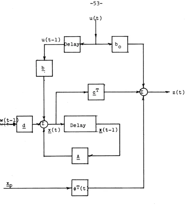
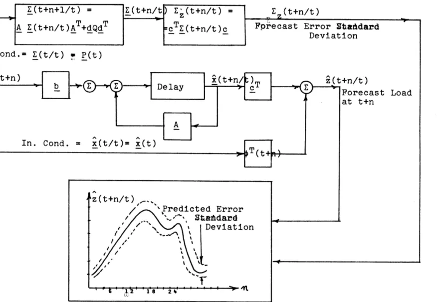
Curves, and Resulting Temperature Deviations, u.. . 41 6. Assumed Stochastic Load Model. . - -.... - .... .

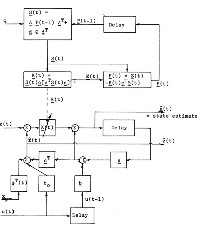
53

7. Estimation of State - Deterministic Load Model. - 54 8. Display of Forecast Load at Time t plus Associated

Error Variance. .. ... . . .. . . . .. .

56

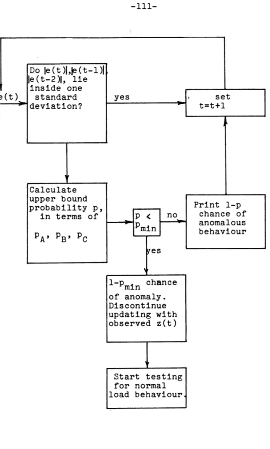
9. Scheme for Testing Abnormal Load Behaviour Based

on 3 Most Recent Residuals.. ... lli 10. Use of e(t) for Anomaly Detection. . . . . . . . . . 112 11. Weighted Least Squares Estimates of Periodic and

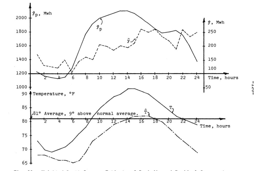
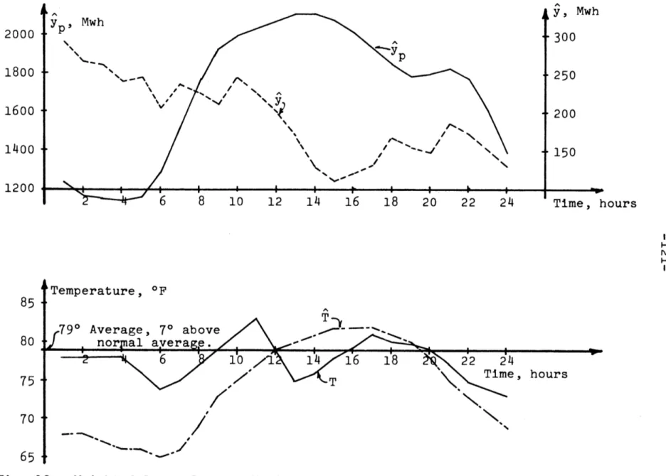
Residual Components - July 16th, 1969. . . . . . . . 120 12. Weighted Least Squares Estimate of Periodic and

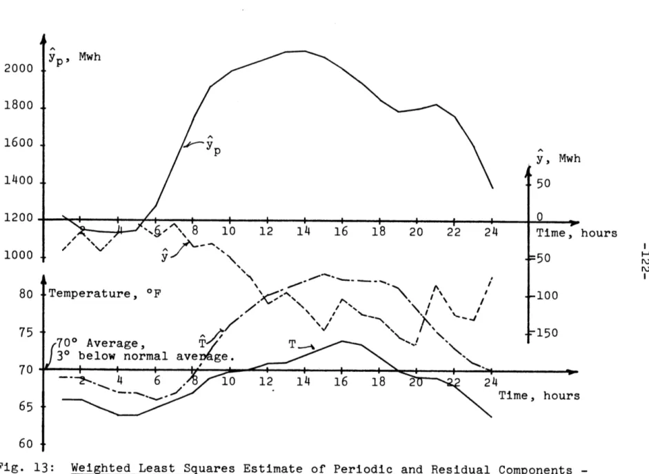
Residual Components - July 17th, 1969. . . . . . . . 121 13. Weighted Least Squares Estimate of Periodic and

Residual Components - July 29th, 1969. , . ... .122 14. Weighted Least Squares Estimate of Periodic and

Residual Components - July 31st, 1969. ... 123 15. Test Filtering of Periodic Component (5 Harmonics)-. 125 16. Result of Prefiltering Load and Temperature

Deviation Data - July 9th, 1969. . . . . . . . . . 127 17. Prediction of Simulated Load - Assuming Model

Parameters Exactly Known, I. . . . . . . ... . . . 138 18. Prediction of Simulated Load - Assuming Model

(9)

-9-page

19. 24-Step Prediction Error for Simulated Load. ....

141

20. One-Step Prediction Error - Anomaly Detection

-Self-Correction

-

Parameters Exactly Known. ....

143 21. Linear Estimation of x

-

Propagation of Standard

Deviationoof

t

Compon~nts, x o and

x

-Simulated Data.

.

147 22. Actual Error in X., and xpl from their True

Values

-

Simulated-Data.

.

148 23. One-Step Prediction Error with Large Initial

Uncertainty in

x_

-

Simulated Data.

.

149 24. Prediction of Simulated Load, Assuming Model

Parameters Uncertain

-

Before Steady State. ....

151 25. Prediction of Simulated Load, Assuming Model

Parameters Uncertain -

In Steady State.

..

....

152 26. Prediction of Simulated Load, Using Identified

Model Parameters

-

Case I. .

.

. . .. .. .

.

154 27. Prediction of Simulated Load, Using Identified

Model Parameters

-

Case II.

.

155 2&- August Load Forecast and Temperature Deviation

-Model np=5, n=m=l. ...

.

.... .... .

160 29. July Load Forecast Error and Temperature

Deviation

-

Model

np=5,

n=m=1.

.

...

161 30. July Load Forecast Error and Temperature

Deviation -

Model np=5, n=m=2.

.

or.

. .. .. .. .

164 31. July Residual Load Forecast and Temperature

Deviation

-

Model

np=5,

n=m=2. .

...

166 32. July One-Step Prediction Error

-Model

np=5,

n=m=2.

..

.

.. . . .. .. .

.

168 33. July Load Forecast Error and Temperature

Deviation

-

Model np=6, n=m=2.

.

... .

. ...

170 34. August Load Forecast and Prediction Error,

I-Model ng=7, n=m=2.

...

.

..

.... ....

.

176 35. August Residual Load Forecast and Temperature

(10)

page

36. August Load Forecast and Prediction Error,

II-Model np=7, n=m=2. ...

.

...

178 37. August Residual Load Forecast and Temperature

Deviation, II- Model np=7, nm2..

...

179

38. Effect of Temperature on Summer Load (CEI). . . . . 181 39. Effect of Temperature on Winter Load (CEI). . . . . 182

40. January Residual Load Forecast and Temperature

Deviation

-

Model ng=5, n=m=2.

.

a. .. . .... .

185 41. January Load Forecast and Prediction Error

-Model ng=5, n=m=2.

..

.

. . . . .. ..

.

186 42. July One-Step Prediction Error

-

Anomaly

Detection & Self-Correction - Model np=6 , n=m=2.. . 189

43. Block Diagram Implementation of Complete

Approach. .

...

... .

...

199 TABLES:

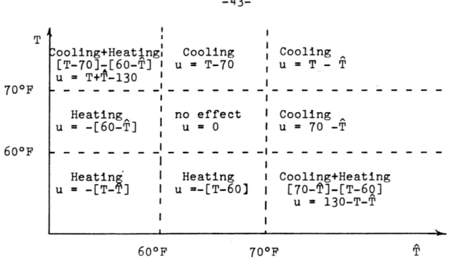
1. Definition of u(T, T) in terms of Actual and

Normal Temperatures.

...

.

...

43 2. Examples of Calculation of Temperature Deviation.

. .

45 3. Simulated Inputs and Corresponding OUtputs for

(11)

-11-I.0 INTRODUCTION & BACKGROUND

I.1 Introduction:

We have two principal objectives in this study.

The

primary aim is to study the problem of short term electric

load forecasting via the concepts of system modelling and

identification, and state estimation and prediction. The

second is to verify the extent of the validity of the

availa-ble theory of system identification and modelling as applied

to a real problem such as load forecasting, and if necessary

and possible extend its range.

We first hypothesize a general mathematical model

for the load of a power system based on physical reasoning

and observed load behaviour under varying conditions. The

main points of this model are the separation of load into

two components, periodic and residual. The first depends on

the time of the day and day of the week, while the reaidual

term is a random process defined as the output of a discrete

linear system driven by white noise and by a temperature

devia-tion variable.

The latter is in turn defined by a non-linear

memoryless function of both actual and normal temperatures.

This is described in sections II.1 through 11.6.

The remaining sections of chapter II describe the

main forecasting algorithms, which are essentially the Kalman

filter-predictor equations (Ref. 11).

The forecasting

techni-que

is computationally simple, and provides the operator

(12)

complement each other and improve the reliability and effici-ency of the operation of a power system. For example, the operator may be given a load forecast for any future time he requests, together with the expected error standard deviation. Alternatively, he may wish to see a display of predicted load values at discrete intervals with the corresponding

statisti-cal confidence level. This display may prove very valuable in scheduling generation and power exchanges.

Another main asset of this approach is the capability of detecting abnormal load behaviour otherwise not so easily notiueable by the naked eye. Under these conditions the ope-rator is warned of the abnormality, and may introduce personal corrections to the forecast if necessary.

Chapter III describes a number of approaches for the identification of the number and set of unknown model para-meters from a past observed data record. A least squares or maximum likelihood approach is used and a number of techniques are described and analyzed. For reasons of convenience, we choose one relying on the Fletcher-Powell algorithms for minimizing functions.(Ref. 22).

Chapter IV describes a number of tests carried out on both simulated and real data to evaluate the proposed model, identification and forecasting techniques. The load data

was obtained from the Cleveland Electric Illuminating Company while the weather data came from the U.S. Weather Bureau.

(13)

-13-The simulated data tests are described in sections IV.1 through IV.5.

Results with real data were very successful and are described in IV.6. Models are determined for the months of July, August and January, each of which yields predictions from one hour to one week compatible with the predicted error standard deviation of from 1% to 2.5% of peak load. The mo-del's ability to predict is particularly emphasized during periods of large temperature deviations from normal, such as heat waves. It must also be emphasized that actual tempera-ture data was used in these predictions. Predicted weather data together with its confidence level can be used, resul-ting in worse load forecasts. The detection of anomalous load behaviour is tested by artificially introducing small disturbances into the load data and proves very successful.

Chapter V proposes a number of guidelines and recom-mendations for the practical implementation of the proposed

technique in a real systeip.

Chapter VI summarizes the work done and makes a num-ber of conclusions and recommendations for future research.

1.2 Background:

1.2.1 General Description of an Electric Power System:

The purpose of an electric power system is to genera-te and distribugenera-te the necessary power demanded by its customers. Furthermore, this must be done reliably and efficiently, that is with a minimum number of power interruptions or

(14)

distur-bances and least cost to the company and the customer.

The satisfaction of these conditions is a formida-ble task which is receiving consideraformida-ble attention. Load

forecasting is but one aspect of this problem, but it is sufficiently challenging and important to merit separate attention.

The electric load is defined as the real electric power demanded by the customers of a power company. This demand varies considerably over a period of 24 hours, so that power generation must be adjusted over this period to follow this variation as closely as possible. Small load changes, those occuring in the order of a few minutes or fractions of,

can be tracked by small changes of generation by the units already in operation. This is the so-called load-frequency

control problem whose main objective is to maintain the fre-quency at 60 Hz, as well as the power flow to interconnected companies constant (Ref.1, 2).

Larger load variations which occur over the period of 24 hours cannot be tracked by the limited capacity genera-tors

already

on-line. Instead, new blocks of generation must be brought into the system, and be ready to supply additional power when demanded. From an economic point of view it makes sense not to start up and maintain unnecessary spinning reser-ve. On the other hand, lack of spinning reserve would neces-sitate shedding of load or some such more drastic undesirable measures.

(15)

-15-A compromise must thus be reached in scheduling

gene-ration to optimize opegene-rational costs as well as system

relia-bility. The satisfaction of this compromise is complicated

by a number of constraints. Some of these are, the delay of

from three to six hours to bring a block of generation up to

running speeds, that is 3600 rpm; relative costs of operating

different forms of generation in the system, e.g. steam, hydro,

nuclear; transmission failure contingency reserve, generation

failure contingency reserve, maintenance shutdowns, power

flow to interconnected companies and others.

It is clear that load forecasting plays an important

part in this aspect of a power system's operation. That is,

economical as well as reliable tracking of the load demanded

cannot be accomplished, in view of the above described delays,

and constraints, unless ample warning time of future load

behaviour is provided.

1.2.2 Observed Load Behaviour:

In this section we discuss load behaviour as it is

known from years of observation, as well as the behaviour of

the consumers under varying time and weather effects.

The load, z(t), is the power consumed at time t by

all industrial, commercial, public, domestic and agricultural

consumers supplied by the particular power system. Generally

these customers are distributed over a large area, e.g. a large

city, or a group of cities, towns and rural areas.

The

beha-viour of z with time is therefore determined by the time

(16)

variation of the myriad of power consuming devices in this

area.

It would then be an impossible task to attempt to

understand load behaviour from the point of view of its

indi-vidual constituents.

A better possibility may be to monitor

chosen buses (network nodes) which serve mainly industrial,

residential, commercial or agricultftral loads and analyze the

behaviour of each such load. This monitoring is however not

available, and one could still have areas which do not fit

any of the above categories.

Nevertheless such studies,

toge-ther with surveys in these areas as to the nature of the power

consumption in them, might be a significant approach in more

ambitious projects.

The load is fortunately a reasonably well behaved

time series and tends to follow recognizable patterns even

when the different types of loads discussed above are not

separated. This regularity is due to the large quantities of

power consuming devices and consumers which tend to smooth

out or average the total load, in addition to the regular

patterns of consumption by the customers and how they are

affec-ted by certain factors such as time and weather conditions.

Nevertheless, the load is an uncertain process in the sense

that its value at any time cahnot normally be exactly

determi-ned, except after it is observed, that is one cannot normally

exactly model or predict the load. The aim of load

forecas-ting is thus to model and predict the load, z, as closely as

(17)

-17-possible in the presence of this inherent uncertainty. Short time load behaviour (up to 5 min.)

If we observe the load over the period of a few seconds to minutes, under normal conditions, small random fluctuations are clearly evident. In addition, we may have

larger longer lasting variations which are significant from the point of view of load frequency control, that is variations which can be followed by the on-line generators. Under normal conditions load changes in this time interval are not large enough to necessitate bringing additional generation into

line.

The small fast fluctuations are generally ig-nored by the load frequency controller as they could not be followed rapidly enough by the generation equipment in addition to normally being sufficiently small to be negligible when compared with the total load.

Daily load behaviour (5 min. to 24 hours)

The load behaviour over a 24 hour period acqui-res considerable regularity. A typical sample over a 48 hour period is shown in Fig. 1.

The most obvious characteristic is that of near periodicity over a 24 hour period. It generally rises very

rapidly in the early morning, breakfast time, stays approx-imately constant over the morning hours and decays slowly after supper time, approximately repeating this cycle every 24 hour period. The reason for this behaviour is quite evident, that is, consumption approximately follows

(18)

-

2000

4 K~t

Li

Avrg

TeprtrIvrg

eprtr

vrg

eprtr

73

0 F

5F7I

Iusa

7/26

/36

Tusa /46

Iensa

12

1

24

6

12

24

6

12

18

Time, hours

Fig. 1: Typical Weekday Load Behaviour (Cleveland Illuminating Co.)

(19)

Load, Mwh

7/26/69

Aver.751F

1600

rW

"

1500

-1400 X 4 ' 7/27/69

4 8/2/69

Aver. 76

0

F

I

Aver. 71

0

F

1300

r

1200

_.A

1100

_r

4

8/3/69

a

Aver. 680F

1000

Saturday

4,

Sunday

6

12

18

24

18 T12 24

Time, hours

Fig. 2: Typical Weekdnd Load Behaviour (Cleveland Illuminating Co.)

(20)

the sleeping, working, resting cycles of its customers,

which fortunately are fairly regular.

Effect of weekday on load behaviour

This basic daily load behaviour may vary from

weekday to weekday to a small extent, given that all

conditions are equal, in a manner not attributable to

the random nature of the process. This is due to small

changes in power consumption habits from day to day,

e.g. from a Monday to a Friday. This difference is much

more pronounced during the weekend days or a holiday

period, for obvious reasons. See figure 2.

Given all other conditions equal, days

separa-ted by multiples of one week will show a behaviour

approx-imately equal, with larger differences appearing as this

interval increases.

Effect of seasons on load behaviour

The nature of the load changes considerably

over the seasons. This is due to variations in weather,

duration of day, and customers' consumption habits. Thus

dubing the winter we may make use of more electric

heat-ing or cookheat-ing devices. Days are shorter hence lightheat-ing

loads increase. During the summer, air conditioning and

refrigeration loads become significant, but lighting

loads may decrease. In addition consumers' habits change,

thus in summer we go to bed later, watch less television,

(21)

-21-and use less lighting.

This seasonal changes in the behaviour of the daily load curve are fortunately slow and can be readily identified. However, although slow, they tend to change the daily load curve from week to week by a non-negli-gible amount.

Effect of years on load

Superimposed on the daily and seasonal patterns of load behaviour one has the inevitable growth factor due to the rapid growth of power consuming devices availa-ble.

Such dffects are however very slow and for the purpose of short term load forecasting not very difficult to take into account. For the purpose of long term

plan-ning of future power system needs this factor is significant. Effect of weather on load

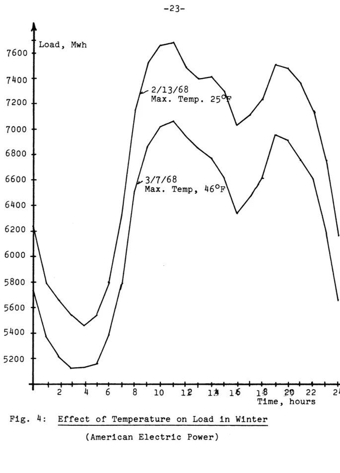
Analysis of daily load curves not too far apart in the calendar, e.g. one week apart, shows that, for the same weekday, weather plays a very significant role in the power

consumption as shown in Fig. 3, 4. The major weather effects which influence the load behaviour are:

i) Temperature

ii) Light Intensity iii) Humidity

iv) Wind Speed v) Precipitation

(22)

Load, Mwh

7400

200

000

800

600

400

200

000 8/19/60

Max. Temp. 89

0

F

8/12/68

Max. Temp.

740F

800

600 1400

200 1000

800

2

4

6

8

10

12

14

16

18

20

22 Time, hours

Fig.

3:

Effect of Temperature

on Load in Summer

(American Electric Power)

(23)

-23-7600

Load, Mwh

7400

2/13

7200

Max.

7000

6800

6600

3/7/6

Max.

6400

6200

6000

5800

56oo

5400

5200

2

4

6

8

10 Fig. 4:

Effect of Temperature

/68

Temp.

8 Temp,

12 1-

2D

22

2 Time, hours

on Load in Winter

(24)

decreasing significance to the load behaviour.

The qualitative reason as to the influence of weather

in load behaviour is quite clear. Our comfort, well-being

and habits are closely related to the weather conditions.

We surround ourselves with a number of electric devices which

we use to maintain these living conditions at comfortable

andAdesirable levels. Thus we have heating and cooling

devi-ces, refrigeration, cooking, cutting, washing, drying devidevi-ces,

lighting, radios, televisions and many others.

The use and

power consumption of all these is to some degree affected by

the nature of the weather, through the consumer.

Clearly some loads are unaffected by weather. These

are industrial and to some extent commercial loads.

In these

cases we have considerable power consumption which is

indepen-dent of weather.

Random load behaviour

In spite of the load's regular behaviour with respect

to time and weather, at any instant of time its value is

un-certain to some degree. This behaviour is clear in view of

the nature of the load. That is, the summation of the power

consumed by literally thousands of devices, each of which is

independently controlled by human beings, introduces inherent

uncertainty in its value. However, because of the large

num-ber of devices involved, some regularity can be expected due

to a smoothing or averaging effect, more or less like that of

throwing a pair of dice a large number of times.

In the case

(25)

-25-of the load the number -25-of possible outcomes is infinite,

time varying and depends on a number of factors both

deter-ministic and uncertain.

This random behaviour may be of the type discussed

earlier, that is very fast and small fluctuations

superimpo-sed on slower larger changes, or it may consist of a large

discontinuity in the load as caused by the sudden gain or

loss of a large load, such as factory or building.

A second form of randomness in the load is due to

disturbances which although not well predictable in magnitude,

can be predicted in time. Examples are effects like the World

Series, Lunar landings, and election days.

The worst cases

of random disturbances unpredictable in both time and

magni-tude are caused by events such as national or loaal

emergen-cies, assasinations of prominent figures, and natural

disas-ters such as earthquakes, tornadoes and hurricanes.

1.2.3 State of the Field:

Load forecasting is still considered more of an art

than a science. For this reason many power companies maintain

a number of load forecasters who base their forecasts on

experience and insight. Basically, they maintain records of

past load behaviour, together with past weather conditions,

industry strikes and any other factor which has been known to

influence the load. Based on this information, forecast

weather conditions for the area, and some other random effects,

a load prediction is made by comparing these conditions with

(26)

those of a day with similar ones, whose load behaviour is recorded in their files. Adding a fudge factor based on insight, a forecast is made which, more often than not, is sufficiently accurate.

The disadvantages here lie in the fact that large amounts of data must be stored, only one or two forecasts are made daily, and the method is highly subjective and therefore

liable to human errors and biases. Alternatively this type of forecast may be advantageous, as the complexity of the problem is such that human insight or intuition may be the best way of arriving at a forecast when conditions deviate

from the normal.

Over the past years a serious attempt has been made to develop mathematical models which could be implemented in a computer for automatic load forecasting. Good surveys on the subject have been written by Mattheuman and Nicholson, and Gupta (Ref. 3, 4).

There are two basic approaches. One is to establish a mathematical model based on the correlation between load and weather, and the second is to base this model on the rela-tioship between the present and past values of the load.

Arguments against weather-correlatidn models have been raised since these req&ire weather data monitoring, as well as accurate weather prediction, leading to the complaint

that companies do not have such monitoring facilities easily available, and that erroneous weather forecasts would lead

(27)

-27-to doubling the load forecast error. Techniques that make

use of past load data only, have the advantage of being

sim-pler to implement in the sense that this data is more readily

available. Other arguments state that the response of the

load to weather effects tends to be relatively slow (of the

order of 24 hours) and therefore easily identifiable and

predictable in terms of the most recent past load data (Ref.

5).

Weather effects with faster responses such as cloud

cover are difficult to predict and therefore are not included.

On the other hand ignoring this evident correlation

would seem to be a rejection of very significant information

abou the load behaviour. The use of past and present weather

would seem to be

very significanttin arriving at better

load forecasts for lead times of 24 hours or more, than those

based only on past load data. The argument being that past

load data does not contain information about the present and

most recent weather effects. In addition sudden changes in

weather conditions could be incorporated into the load

fore-cast.

Also some correlation exists between the most recent

weather and the present load, so that weather forecasts even

if inexact should yield better forecasts than if altogether

ignored. Finally, a weather dependent model can serve to

carry out contingency predictions for different weather

forecasts.

(28)

Weather correlation techniques

Work on load models based on weather correlation has

been done by Dryar, Davies, and Heinemann (Ref. 6, 7, 8).

The basic approach is to find a deterministic relation between

the peak load and the average daily weather effects considered

significant. Davies utilizes average temperature, wind effects,

illumination index and precipitation index. Heinemann uses

a similar approach but introduces a "dynamic effect" due to

"heat build-up". In his model he considers a relation between

load peaks now and average weather effects for the past three

days.

These effects are wet and dry bulb temperature as well

as relative humidity.

These techniques are limited to the modelling of

load at fixed points in time or to peak loads.

Load variations

with time of day are not considered, neither do these

techni-qnes provide a measure of the uncertainty associated with

the prediction.

Load correlation techniques

This approach is favoured by some authors as discussed

earlier. The jist here is to make use of the most recent

load data to extrapolate in some sense into the future.

The more significant contribution along this line

is made by Farmer and Potton (Ref.

5),

who also introduce a

probabilistic structure into the load model. Essentially,

load observations over a period of six weeks in the past are

used to estimate the value of the autocorrelation function of

(29)

-29-the load. A finite Karhoum-Loeve expansion based on the found autocorrelation function eigenvalues and vectors is then used to model the load. The parameters of the expansion can be recursively updated to best fit the mosr recent

observations.

This approach provides the user with a continuous forecast and error standard deviation rather than just fore-casting a few values during the day. It is however limited to the length of time it can accurately forecast by the fact that it does not consider weather effects. In addition, under varying weather conditions it is necessary to reevaluate the model eigenvectors, a task of considerable complexity.

A similar approach is attempted by Christiaanse (Ref. 9). He models the load behaviour at intervals of one hour by a time series of periodic functions with a period of one week. The free parameters are recursively updated by new observations. The advantage of this technique lies in its relative simplicity of implementation, however it contains the inherent drawback of not describing the effect of weather separately. Thus during fast changing weather conditions or periods of heat or cold, the model weakens.

Toyoda et al. (Ref. 10) suggest a state space model which incorporates both the effect of weather, temperature

and humidity, as well as the effect of the latest load obser-vation. This approach is somewhat similar to the author's, however we attempt to incorporate more complexity into the

(30)

model and make considerable use of adaptive identification

techniques to estimate the parameters of the model dynamics

rather than assuming that these are apriori known. In

addition we verify the validity of the technique with real

data experimentation.

I.2.4 Important Factors in Load Forecasting Techniques:

Based on the results obtained by the various authors

it is possible to arrive at a set of significant objectives

one should aim for in designing a load forecasting technique.

The two primary aims are the accuracy and length of

the forecast and the complexity involved in evaluating the

forecast. Generally the industry leans toward techniques

which are readily implementable on-line, i.e. will not burden

the availabi& computer excessively.

Accuracy of forecast

is a more obscure objective, exact numbers depending on the

particular company's operational objectives. This criterion

is also closely related to the length of the forecast.

Shorter prediction times result in better accuracy, but

predic-tion times of 24 hours or more can cause errors to

deterio-rate badly unless we go to more complex techniques.

As mentioned above techniques which collect and

process data on-line to update the forecast are desirable.

A technique, in addition to being accurate, should determine

the extent of the model's confidence in the forecast or an

estimate of the prediction error. This would provide us with

a quantitative criterion to decide if the model has failed,

(31)

-31-that is, to detect anomalous load behaviour.

Since exact models are a practical impossibility, it is desirable to have a feedback type scheme for on-line corrections of forecasts as new observations are made. This will reduce the sensitivity of the forecast to modelling errors.

Finally, the model should be adaptible to seasonal variations in the load behaviour without drastic model changes, by for example adjusting a number of parameters. This would allow us to minimize the number of models which would have to be stored to be used under varying conditions.

(32)

II.0 PROPOSED LOAD MODEL & FORECASTING TECHNIQUE

II.1 Preliminary Remarks:

In this chapter we develop a mathematical model for

the load of a large power system. This modelling step is

based on the observed behaviour of a typical load curve under

varying conditions, the behaviour of the consumers under the

same conditions, as well as pure assumption. The modeliis

kept as simple as possible at the same time incorporating the

main hypothesized structure and different effects.

A number

of free coefficients parameterize the model, their exact

value to be determined by model fitting techniques, that is

system identification.

In addition, we describe the estimation-prediction

algorithms which are used for on-line forecasting. This is

essentially a Kalman estimator-predictor scheme (Ref. 11).

11.2 Load Modelling Concepts:

We are dealing here with a time varying process which

is inherently uncertain. Its value at any one time is

direc-tly determined by the customers who turn 'switches on and off.

These are in turn influenced by a number of factors such as

weather conditions and living patterns to use electricity with

a certain regularity. Since we are dealing with a very large

ensemble of people it is expected that these various

influen-cing effects will be felt in the load in some systematic or

regular way.

Indeed, observations show that such regularities

exist.

(33)

-33-We wish then to describe these regularities mathema-tically as simply as possible, yet including as many effects as considered significant.

The choice of a right model is very important if we wish it to be valid for future times and forecast accurately. There is however little more one can do at this stage except justify the model structure based on the underlying basic laws of the process, and experimentally verify its validity. If it should not be accurate, the identification step would give us an idea of how to alter the model, by suggesting that additional variables or non-linearities may be needed.

11.3 Load Model Structure:

The hypothesis is made that the load, z, at any time of the day, t, can be expressed as,

z(t) = yp(t) + y(t) (2.1)

where yp is a periodic component and y is a residual term. The assumption is made that yp is dependent only on the time of the day and the day of the week. We will also assume that yp is a deterministic process, so that its exact value is determinable from its model.

The residual term, y, is assumed to be an uncertain process, time varying and correlated with itself over time as well as with certain weather effects.

Again it should be emphasized that this is simply a model which makes sense from the point of view of load and customer behaviour, that is underlying influencing factors,

(34)

yield better results.. We stick to the concept of first trying the simplest model form and work from there.

The existence and structure of yp and y are now jus-tified and described respectively from a heuristic point of view.

11.4 Periodic Component:

This component attempts to describe that part of the load behaviour which depends only on the time of the day and day of the week.

That this. component exists is justifiable in terms of the total observed load behaviour. Thus the load daily goes through a 24 hour near-periodic cycle which rises in the early morning, reaches a peak at mid-morning, may dip and rise again until the late afternoon drop, rising again during the evening, finally dropping considerably at night.

This approximate behaviour is consistently repeated, exhibiting similar rises and falls at approximately the same hours. _{In addition the shape of this characteristic curve} is essentially unaffected by changes in weather conditions. In the examples of Fig. 3 and 4, this behaviour is seen. That is, for considerably large variations in temperature, the

magnitude of the load is affected but its structure with time stays approximately the same.

(35)

-35-The behaviour of y p with the day of the week is also observable. Distinct differences in the daily load behaviour occur over the weekdays and in particular over weekends and holidays. Slighter differences also occur between the same weekdays separated by various week integers, especially over

the seasons.

The existence of this component can also be justified from physical reasoning. The daily behaviour is clearly attri-butable to the consumer habits of power consumption centered abou their 24 hour cycles of sleep, eating, work and rest periods. Thus in the morning residential, commercial and

industrial consumption pick up very rapidly. After noon time, there may be a decrease due to smaller residential loads, and as commercial and industrial loads decrease. A rise is again encountered at supper time due to cooking, lighting and tele-vision loads, which rapidly decgys as people turn in.

The webkday variations can also be explained on this basis. Thus the cyclic daily consumption habits may be sligh-tly different over the wetkdays, and certainly over the week-ends and holidays when industrial and commercial loads are mainly off.

The change in behaviour during longer time periods

is again due to small accumulated changes in consumption habits, changes in eating and sleeping habits over the year. In parti-cular during vacation periods, considerable changes in load consumption may occur.

(36)

The assumed independence of yp for short periods of

time with weather conditions is based on the reasoning that

the "normal" consumption habits which yp describes are not

affected by weather as suggested in Fig. 3 and 4. This is due

to the fact that when weather conditions deviate from normal

then the weather sensitive load is excited beyond a normal

level which is itself assumed unaffected.

Any deviation of the load from its normal level,

whether due to weather deviations from normal or due to random

effects, will be modelled by the residual term, y.

The periodic component of load, yp, is therefore a

hypothetical deterministic process which is justified on the

basis of observed load near-periodicity. The residual term,

y, is in turn another hypothetical process whose structure

will be discussed below. Their existence will be more

defini-tely justified after experimental testing of the model with

real data.

The structure of the periodic component, yp, can be

expressed as a time series,

n

Yp(t)

=

x

+

LTx' sin[2w1i/24]t+xnp+icos[2wi/24]t) (2.2)

i=1

which we can rewrite in vector form as,

yp(t)

=

*T(t)

x

(2.3)

where defining,

(37)

-37-then,

1 sin

wot

f(t) = sin npWot (2.5) Cos mot cosn _{np Wt.} 0

xP

xp

(2.6)

x

2np

- p

-while t stands for the time of the day.

The vector

p

is assumed constant,however as

sugges-ted earlier small variations over the weekdays are possible.

These are particularly noticeable on Saturday and Sunday.

In

this study we first consider three sets of

x,

one for Monday

through Friday, one for Saturday and one for Sunday, but later

experiments indicate that a separate Monday model may be

desirable.

Over the span of two or three weeks the value of

xp

may remain constant for a given weekday, but since normal load

consumption does vary over the seasons we will expect that

xP

should vary accordingly. For these reasons this parameter

will require periodic readjustment, for example once a week.

(38)

The number of elements in the vector

xP,

2np+1, is

presently uncertAin, its value to be determined by

identifica-tion techniques.

However it will later be shown by

experimen-tation to lie between 9 and 15.

11.5 Residual Component, y:

Under "normal" conditions our model would say that

the load, z, should equal the periodic component, yP.

These

inormal" conditions are however highly hypothetical since the

load is never exactly periodic. Thus even if all the weather

effects considered significant are at their normal level, it

is reasonable to expect a random variation around the

perio-dic behaviour. This random variation is provided by the

residual component, y, which we assume to be a random process

depending on the deviations of significant weather variables

from their normal level. More about this dependence will

follow.

The significant weather variables are those that

influence the behaviour of the load. These are in order of

significance (Ref. 12) temperatere, humidity, precipitation,

light intensity, and wind speed, respectively denoted by T,

H, P, L and S. These variables have different influences

depending on the region and power company.

Temperature is the single most important effect as

a great portion of the load is temperature sensitive, e.g.

refrigeration, heating and ait-conditioning. This is

(39)

-39-of T is to increase the load with its increase, but this beha-viour is reversed during the cold months. The remaining

variables have similar effects, all of considerably less impor-tance, the exact value being difficult to establish, depending very much on the specific company.

The problem with analyzing the effect of weather con-ditions other than temperature is the difficulty in obtaining

significant data. For example, wind speed, precipitation and light intensity may vary considerably over the area of the power company affecting certain portions of the load more than others. Such data is not presently available.

Temperature and humidity are much more uniformly

distributed over the load region and can be periodically moni-tored without great problems. In addition this data is

readi-ly available from the weather bureau.

Intthis study we restrict ourselves to the effect of temperature only for simplicity's sake, but its extension to other weather effects could follow along similar lines in more ambitious investigations.

11.5.1 The Effect of Temperature:

In this study we try to analyze the effect of the temperature profile with time on the load, rather than that of some average daily temperature. The reasoning being that different temperatures duting the course of the day will cause the load to behave differently even if the average daily tempe-rature stays normal.