1
Kevin N. Otto*
Center for Innovation in Product Development Massachusetts Institute of Technology
Cambridge, MA 02139
Abstract
This paper presents an approach to determine the proper number of levels required on independent product architectural attributes, given their ability to generate added revenue through more direct targeting to smaller segments, and given the added costs of doing so. This is done in as simple and readily implementable manner as possible, making use only of conjoint data and cost estimates. From this, the order in which to consider added breakouts across the different attributes are prioritized. From this, for any minimum level of profit worth
considering, a set of attribute levels to offer on each architectural attribute can be selected. Then, for any selected set of attribute levels to offer, the most effective product family using those levels is determined from the
permutations.
*
Corresponding Author : 77 Massachusetts Ave, Room 3-449B, Cambridge, MA 02139. [email protected]
Introduction
Product families based upon a common product architecture are often used in many industries to leverage the common systems while yet tailoring some aspects of a product to more adequately match the product with a customer’s application. Yet, even in industries with very slow technology and market change rates, known demand volume, and known costs, there is no formulation of the optimal portfolio architecture to maximize profit. In this paper, we develop this formulation, given market variety demands as modeled through conjoint data and complexity cost coefficients for added levels of offering on attributes.
The formulation presented requires data with modest requirements to develop or estimate. We derive our model from basic assumptions about both the market and costs of production/development. From the derivation, a methodology is developed with two fundamental analysis components. First, for a given minimum profit level to bother with, the best permutative set of architectural attribute levels is determined. Then, when restricted to this set of levels, the product family constructed from that set that most effectively meets the market demand is determined. We operate with independent product architecture attributes. Two architectural attributes are design-independent if the numbers of levels to offer of each does not impact the design of the other. For example, when system architecting an automobile, the passing acceleration, interior price, and seat height are design-independent. On the other hand, primary customer need variables such as towing capacity and passing acceleration are not, since both depend on the design choice of engine size. Engine size and vehicle weight are design independent (though perhaps there are rough interval constraints between them), and cover the concerns of passing acceleration and towing capacity. Design independence is fundamentally concerned with and determined by the product architecture, not on any statistical market considerations. Design independent variables are the ones that the initial systems engineering of a product family must operate with when determining numbers of levels on architecture attributes. The traditional approach to determining the variety content capability of a product family architecture is to qualitatively flow down variety requirements from a market segment attack approach. That is, a marketing group determines segments to attack, and defines ideal product attributes for each segment that should be constructed. Typically, this does not consider design, production and supply chain constraints, and so a negotiation ensues to define the actual product attributes. Our approach here is to do these activities quantitatively. We do this in two steps using the underlying market data – first we determine the number of levels on each attribute, then second determine the offered family from this set.
To understand this, consider the more common market segment attack approach. Analytically, the idea is to develop conjoint data of market share, cluster analyze it to define market segments, the centroids of which generally define
architectural attribute targets for design teams. Unfortunately and commonly, however, this gives rise to excess product architecture complexity. For example, consider two attributes. An effective segmentation may result in three clusters, and so three products are to be developed, each with three separate sets of architectural attributes. This generally forces the design team to develop a product portfolio capable of 9 permutations of the architectural attributes – 3 levels over 2 attributes. Therefore, with this approach, excess complexity enters. Further, the product portfolio tends to grow, since the platform design can relatively easily accommodate the nine product
configurations, they are often offered, when in fact seven are not particularly worthwhile. The result is that companies offer overly complex product families, when a smaller set of levels on some architectural attributes would have been more profitable. Documented common examples of such product proliferation include film (Jaime, 1998), electronics assembly (Mosher, 1999), photocopiers (Zamirowski, 1999), vehicle option content on everything from rear end differentials to interior content (Roberson, 1999), and commercial aircraft models (Weir, 2000), among many others. No industry has an effective set of analyses to simultaneously manage both revenue from variety and costs from complexity.
Related Work
The development of product families built on product platforms and shared modules has been the subject of much recent research. Meyer and Lehnerd (1997) have done extensive case studies on platforms, pointing out their advantages and challenges, and demonstrating their ability to save costs.Other researchers such as Sanderson and Uzumeri (1995) and Henderson and Clark (1990) have also shown that the use of platforms has given companies an edge on the number of products they can offer and on their profitability over their competitors. Other management research has shown different approaches on managing the planning and use of platforms (Wheelwright and Clark, 1992; Erens and Verhulst, 1996; Robertson and Ulrich, 1998; Pedersen, 1999; Pulkkinen et al., 1999).
To determine marketshare for various products, conjoint analysis has long been studied and developed. Ben-Akiva and Lerman (1997) provide a useful reference for conducting conjoint studies, as does Urban and Hauser (1993). Sawtooth Inc. (2000) has multiple software tools for forming conjoint studies to question customers to determine buying preference structures, to which product attributes and positioning can be optimized. These works, however, ignore the costs of offering the combinations of levels on each attribute. For example, to meet three different products over 2 attributes, often three levels are demanded on each attribute, resulting in an architecture that is actually capable of nine different products. Portfolio complexity thereby grows. On the other hand, conjoint studies do provide a good estimate of marketshare, given the utility functions of a representative sample of the market. Given a set of offerings, software models exist to calculate market share, based upon the orderings of the offerings for each sample point (customer) in the market model.
Most related to the work here are efforts to determine a most effective set of product offerings, given conjoint data. Moore et al (1999) consider conjoint data and cost coefficients for each attribute to offer multiple levels. They consider whether to platform a variable (1 level) or not (multiple levels), and rank order the attributes. In this work, we extend these thoughts to multiple levels and define a break out sequence.
In the engineering design literature, one can find several design and manufacturing strategies for offering variety that begin with commonality metrics (Martin and Ishii, 1997; Kota and Sethuraman, 1998). Krishnan et al. (1998) developed network models to design families of products that are measured along a single performance criterion. Optimization approaches have been developed by Gonzalez-Zugasti et al. (1998) and Nelson et al. (1999) to design product platforms and families of variants. Another optimization approach is used by Fujita et al. (1999) for designing a family of products from catalogs of existing swappable modules. These approaches are all downstream component form development exercises as compared to the portfolio architecture work here.
We next develop an analysis to define the profit extractable from any choice of levels on architectural variables. We do this by first developing a revenue model, subsequently a cost model, which then defines a profit model. Then we develop this into a method to analyze the profit capability of any breakout choice. Given this choice, we then define the portfolio to offer from the set of level permutations.
Profit from Variety
Determining the ideal family based upon profit maximization will involve two different models, a revenue model based upon conjoint data, and a cost model based upon cost-of-complexity factors of production.
Revenue from Variety
Revenue from a Customer
Consider a market S of customers sk. Define the price that customer k will pay as a function of desired architectural
attribute levels τik as Pk, where each architectural attribute is denoted xi. Expanding Pk in a Taylor series about τk v ,
(
)
∑
(
)
∑
− + ∂ ∂ + − ∂ ∂ + = = K v v v v 2 2 2 0 2 1 ) , ( ik i i ik i i k k k x x f x x f P x f P k k τ τ τ τ τ (1)where P0k is the maximum that customer k will pay, and only when the product configuration is exactly at τk v . Now, k i x f τv ∂ ∂ = 0, (2)
since Pk is at a local maximum at τk v
. Therefore, to second order,
(
)
∑
− ∂ ∂ + = 2 2 2 0 2 1 ik i i k k x x f P P k τ τv . (3)The higher order effects that cause (3) to vary from (1) primarily arise for two reasons: highly nonlinear fall off of price with variance of an offering from the individually desired target, and coupled variables that cause rotation of the parabolic surface. That is, while the variables may be design independent, they may not be price independent to customer k, causing rotation of the price surface. Nonetheless, (3) is effective for thinking about the primary mode of price fall-off: deviation from individually desired targets. For more complex pricing models, non-linear and rotated variables can be applied as necessary. Rewriting (3) with the partials as relative weighting variables,
(
)
∑
− − = 2 0k ik i ik k P W x P τ . (4)This is the standard ideal point preference model (Ben-Akiva and Lerman,1997).
Market Revenue
Now for the entire market S, consider when the design team must choose a single set of architectural targets *xv to make the most revenue. For any choice of architectural targets xv, the revenue will be
(
)
∑∑
∑
∑
∈ ∈ ∈ − − = = S s i ik i ik S s k S s k k k k x W P P x R(v) 0 τ 2. (5)Then, the maximum revenue generating solution is
(
)
∑∑
∑
∈ ∈ − − = S s i ik i ik x S s k k k x W P x R(v*) 0 infv τ 2 . (6)That is, the solution to picking architectural targets *xv is to choose the ones that minimize market variance over the coverage space S. For normally distributed τik data, one can derive that the solution to (6) is when
µv
v
=
*
x , (7)
the average of each architectural attribute over the market. This is fundamental – that a design team should pick targets that minimize market variance – and it simply presumes a quadratic loss model for each customer, and that one should not position products with respect to the competition.
The maximum extractable revenue with that one average offering will be
∑
− = i i i W R R* 0 σ ,2 (8) where∑
∈ = S s k k P R0 0 (9)has interpretation of the maximum possible revenue extractable from the market, if each customer sk was given their
mass-customization solution xk v
∑
∈ = S s ik i k W W (10)is market-average squared importance coefficient for architectural attribute i.
At this point it is worth making an argument over choice of variables. This is a reduced preference model – an attempt to fit marketshare directly to architectural attributes. In the marketing literature, this is only suggested for so-called primary variables from customer interviews. That is, only the main descriptor variables that customers use to describe a product should be used to fit marketshare, since most others (more architecturally detailed variables) do not fit well, due to poor correlation and lack of fit. While the fitting problems may be true, what this does is push the fitting problem off to the design engineers. The market model fits marketshare well to primary customer need variables, but then the design engineers must estimate some kind of mapping between the primary customer need variables and the architectural attributes they must make decisions over. Often, the House of Quality or some similar qualitative approach is taken, but this is hardly a validated quantitative equation relating levels of the architectural variables to levels on the primary customer needs. As such, effective choices on the architectural attributes are not made.
Note therefore that it is irrelevant to think about other descriptor variables of the market for purposes of determining the architectural attribute targets *xv . For example, it is irrelevant that other rotated or mapped spaces provide better fitting models of market revenue. The architectural attributes are what the design team must use to make architecting decisions – using any other variables would force the team to un-transform the conjoint space into the architectural attribute space to make their architecting decisions. It is the variable set that the design team must operate with. For example, a vehicle design team may be able to offer two engine sizes and two vehicle lengths. Coupling these as one variable for improved statistical fitting purposes does not get around the fact that the design team must decide on levels of engine size and levels of vehicle length, and these two variables are
design-independent architectural decisions.
Conjoint Data
Consider using architectural and external variables such as price discounts to partition the entire market S into well-identified market segments Sj. Using these, one can form conjoint studies and query market samples to form
customer preferences (utilities). Alternatively, one could also model the market through market sales data. That is, rather than sampling the space of customers S directly, one might model S by examining past sales as conjoint data. The previous sales volumes on product models yl now form our market space S. This implies the typical issues
when using conjoint data as a surrogate of customer questionnaires, such as the market being relatively stable, the set of entries in the conjoint being comprehensive of the market (including competitor data), and that the variety of products on the market reflects the variety that the market desires.
In either case, the most effective transformation of the entire data into the best fitting model can be applied to partition the market S into segments Sj, for some number J of segments worth attacking. Given this partitioning, to
each subspace Sj one can associate the actual architectural attribute levels for each product in that subspace. The
result is J subspaces of S, each complete with a set of τil statistical data on each xi, where we now index l over the
products sold to the space S, and include marketshare weightings, or over the number of customers in the market. This covers the market S through market selling statistics or through questioning each customer sk.
The result is, we have ideally partitioned sub-markets Sj to which equations (6) – (10) can be applied, to define
product targets xvj*=µvj. Explicitly, for the products yl in each segment Sj, the basic revenue model is
(
)
∑ ∑
∈ − − = i y S il i l i j l x f W R x R( ) 0 τ 2 v . (11)where now τil is the architectural attribute level of product yl on architectural attribute xi, and fl is the marketshare of
product yl. (5) has a solution
(
)
∑ ∑
∈ − − = i y S il i l i x j l x f W R x R( *) 0 infv τ 2 v . (12)Independent of cost considerations, (6) – (10) imply a breakout ordering to the architectural attributes. One can consider only 1 offer xv*=µv, the mean of each attribute across the entire space of sales S. Then, one can partition S
into 2 segments, and evaluate the impact of breaking any architectural attribute into two levels through the relative increase in revenue
(
i21 ( i22a i22b))
i i W R = σ − σ +σ ∆ . (13)where σ is the variance of architectural attribute i across segment j. One should break out into 2 levels theij2 attribute i which has maximum increase in revenue ∆Ri. Similar analysis holds for each subsequent breakout into
higher levels, j = 3, 4, 5, ... That defines the means to define a portfolio with maximum revenue generating capability through minimal increases of complexity. This is true provided the costs of such breakouts are the same for each architectural attribute. Otherwise, cost factors must be considered.
Costs of Complexity
Costs increase with added platform complexity, since increased levels on architectural attributes cause further development problems, production logistic problems, and procurement/supply chain problems. For any architectural attribute model, we can consider cost as being a fixed baseline amount, plus added cost variable with the number of levels offered, plus added cost variable with the deviation of each target’s performance difference from the baseline performance. That is,
∑
∑
− + − + = i i ik i i i i k C M x x C 0 (# 1) α ( 0), (14)where C0 is the fixed cost of the family, Mi is the cost increment for adding an additional level on architectural
attribute i, αi is the cost gain with a unit increase in performance of xi from xi0, a baseline performance of
architectural attribute i. xik is the value of xi in the product purchased by customer k. Note that xik is not necessarily
the target τik; rather xik is what customer k actually purchased, and must be one of the values offered for xi. Note that
xi0 is simply a baseline used when evaluating C0, such as the cheapest offering. It is not necessarily the level offered
with only one level on architectural attribute i.
C0 is the fixed cost associated with developing, producing, distributing and selling a single product x0 v
. Mi is the
cost with adding another offering level on architectural attribute xi. Typically this is composed development and
production/logistic costs. αi is typically composed of the cost gains due to product material changes from xi0.
Profit
To develop a portfolio sizing model considering profit, revenue from variety and cost of complexity must be combined. Generally, the profit Pk extractable from any sale is
k k k R C
P = − . (15)
Summing this over the market space S for any set of offered levels {xi} defines the extracted profit.
) ( ) 1 ( ) ( min }) ({ 0 0 2 0 i i i i i S s i ik ij J j ik S s k i x x N J NM NC x W R P x P k i k − − − − − − − = =
∑∑
∑
∈ ∈ ∈ α τ , (16)where there are Ji levels offered on xi. Again, rather than summing over the market of customers, one can transform
this into a conjoint space by summing over the set of products currently offered in the market as in (11) and (12): ) ( ) 1 ( ) ( min }) ({ 0 0 2 0 i i i i i i y S il ij J j l i i R W f x NC NM J N x x x P l i − − − − − − − =
∑ ∑
∈ ∈ α τ . (17)Maximizing this over the number of possible levels Ji and over the space offered {xi} defines the set of levels to
offer on each architectural attribute. This is a fundamental result for sizing a product portfolio, and again is based upon data that is generally readily available.
Two cases provide special insight into the formulation, the case of a single offer and the case of negligible performance cost gains αi.
Single Offer
With a single offer, we can determine the profit extracted from the market as
(
)
( ) ) ( 0 0 2 0 i i i S s i ik i ik S s k x x N NC x W R P x P k k − − − − − = =∑∑
∑
∈ ∈ α τ v . (18)where there are N customers in S. The configuration *xv to offer is the one such that
(
)
− + − − − =∑∑
∈ ) ( inf *) ( 0 2 0 0 i i i S s i ik i ik x W x N x x NC R x P k α τ v v , (19)which in general no longer results in xv*=µv as in (7). Instead, xi* will back away from the mean in the direction of
the sign of αi. It is more profitable to make offerings that are less costly and slightly off from what the customer
demands on average. Further, an optimization is required to solve for these *xv .
Practically, we find (19) is an effective formulation to solve for targets *xv for any selected subspace Sj, on
architectural attributes that can be easily adjusted.
Flat Cost Gains
As another context, consider when the cost gains αi for architectural attribute level changes are negligible compared
to the cost gains Mi for added numbers of levels. That is, the architectural attribute changes are easy to provide
multiple levels in terms of changing product material, but it is difficult to expand the development and production facilities to accommodate multiple offers. In this case, (16) reduces to
) 1 ( ) ( min }) ({ 2 0 0 − − − − − =
∑∑
∈ i i S s i ik ij j ik x NM J W NC R x P k τ v (20) and once again the solution is to use the cluster means, xvj*=µvj, for any partitioning into levels Ji. That is,) 1 ( }) ({ = 0 − 0 −
∑ ∑
2− i i− i j ij i NM J W NC R x P v σ (21)(21) provides a simple and effective means to determine an maximally profitable portfolio size. That is, one can consider a single offering for the market. As before, the profit extractable will be
∑
− − = i i i W NC R x P( 1) 0 0 σ21 v (22) One can similarly evaluate (21) at any number of partitions J. What is important to compute, though, is the profit increase that will occur when offering more levels to any attribute i. To determine this, evaluate µij and σij for eachsegment at several levels of partitioning J. Then evaluate the profit increase margin for each architectural attribute, through i J j ij J j ij i i W M P i i − − =
∑
∑
+ = = 1 1 2 1 2 σ σ ∆ (23)One should expand the number of levels Ji on the architectural attribute i for which this is maximum. This is
repeated for each additional breakout, thereby defining a breakout sequence – which architectural attributes to expand into an additional level of offering, and in which order among the architectural attributes. This is the fundamental result of the paper.
Limitations
At this point, it is again worth pointing out the limitations of the formulation. While beneficial due to the inherent objectivity, there are caveats, particularly due to the use of conjoint data. First, the conjoint data must be appropriate for specifying the new product architecture. There are two concerns here, that the data is complete and that it is representative.
The conjoint data must be comprehensive of the sales of all products in the entire market the new architecture is intended to cover. In particular, competitor conjoint data is required, both in sales volumes and architectural attribute data. If only internal sales data is used, a family will result that most easily replaces the previous sales and goes after no additional competitor sales.
The conjoint data must be representative of the new market that the new architecture is intended to attack. This means the market must be slowly changing – the past sales data must be representative of future sales. This can be a tenuous assumption in some markets, such as high technology content markets.
The conjoint data must be representative of sales that can be attained. In particular, this models ignores effects of competitor actions in the market. If a competitor has an offering near one offered, the profit will be less. This analysis incorporates no competitor modeling, where one might downgrade the revenue generated by any particular market segment due to competition. Rather, this model assumes that one will make offers across the entire market, no matter what the competition does.
Finally, if sales data is used instead of customer interviews to represent market preference, the sales data must be complete. Most permutations of the architectural attributes need to be offered on the market so that sales volume impacts of each attribute can be estimated. Often this is difficult, and so customer questionnaires are needed. Independent of the conjoint data parameters, the cost coefficients Mi must also be estimated. These are not the
percentage cost contributions of each attribute to the product, but rather the development/production cost increases when offering additional levels. Estimating these numbers often involves estimating logistical costs within a plant and/or within product development activities, as well as the added material costs. While ideally the development and production facilities would maintain information systems capable of providing such time and cost data, often this is difficult. In such cases, we have found comparative estimates can be made. Picking one attribute as a reference, the comparative increase or decrease in difficulty to offer multiple levels of the other attributes can be estimated. These can be normalized against the variable costs of running the plant to determine cost coefficients. Despite these concerns, though, we have found that the conjoint approach here is worthwhile for its very
objectiveness. The architecture that most can most profitably cover the past sales is worth determining, even in rapidly changing environments. If one knows the direction the market is heading, one can always expand the determined levels appropriately in that expansion direction, using the same estimating approaches as before.
Product Family Definition
The analysis above provides the means to define a most profitable product family for a fixed market with no competitive positioning strategies. The approach is as follows:
1. Develop a statistical dataset of products on the market, with marketshare, price and architectural attribute levels 2. Estimate Wi through regression, sensitivity analysis, or estimation
3. Cluster the dataset into clusters of size 1, 2, 3, 4, … 4. Determine µij and σij for each cluster
5. Estimate Mi through time/cost production data analysis or estimation
6. Evaluate the best breakout sequence using (23)
7. For any set of architectural attribute levels, determine the subset of the permutations to offer as a family We discuss each of these steps next.
Conjoint Analysis
The first step in the process is to collect marketshare and architectural attribute level data on all products in the market, including competitor data. This data should then be analyzed to determine each architectural attribute’s contribution to revenue, Wi. This is not particularly simple, since it involves finding and least squares fitting a non-linear equation of product model revenues R in terms of their architectural attributes xi. This can be difficult to fit.
Almost certainly, a simple quadratic model will not fit well due to coupled attributes. If a well-fit model can be determined, then Taylor series expansion can provide the desired coefficients.
Another approach is to analyze the breakdown of revenue variance with architectural attribute variance. The architectural attributes causing high revenue variance have larger Wi. This is readily accomplished with an ANOVA analysis of the architectural attributes contribution to revenue. Simple linear ANOVA, though, would underestimate the contribution, since this would determine only the direct linear contribution of xi to revenue, and
not higher order and interaction terms.
Alternatively, Wi can be estimated. One such model is 2 1 i i I R W σ = , (24)
where R is the total market revenue, I is the number of attributes, and σi1 is the total market variance of xi. This
provides equal weighting to all architectural attributes, and states that with a single offer, limiting each architectural attribute to one value provides the same percentage contribute to revenue loss. If customer importance ratings are available from questionnaires or the ANOVA studies, (24) can be modified to
∑
= i 2 1 w w R W i i i σ , (25)where wi is the average importance rank of xi. This approach assigns revenue increases for each break out on a
variable according to the variety reduction in the marketplace (as the new standard deviation over the full market standard deviation), as weighted by the customer importance.
These Wi are fixed averages over the entire market. One could refine this to consider averages over sub-spaces Sj.
Indeed, the revenue surface fitting approach could also be similarly fit only on subspaces. At some point, one runs into a lack of data, however. We have found (25) works well, especially given this is intended for preliminary architecting decisions.
Cluster Analysis
Next, the dataset of products should be clustered into segments, for 1, 2, 3, 4, … segments. This can be done with clustering algorithms such as Ward’s method, and by clustering upon the each architectural attribute. Then for each cluster, the means and standard deviations of each architectural attribute should be calculated.
Breakout Table
With an estimate of Mi for each architectural attribute, all required information is attained. This can be summarized
in a breakout analysis table, which lists as columns the increase in revenue, cost, and change in profit with each increase in level, for each row-listed attribute. For any breakout level of profit change, one can then examine the table to determine how many levels of each attribute should be offered. That is, for a profit change of ∆, some attributes will solve (23) at 2 levels, others at 1 level, others perhaps at 8 levels. Thus, for a minimum level of profit to bother with, the number of levels of each attribute is determined. Further, for a market with no competition, the architectural attribute target levels to offer are the segment means µij for each attribute, with j at the level determined
by ∆. This will be explored in detail in the example.
Breakout Sequence
Given the breakout analysis table, one can explore a range of possible ∆, and observe how the breakouts expand. With a high breakout level ∆, no attribute can attain that level of profit change and so all architectural attributes are fixed at 1 level. As ∆ is lowered, at some point one architectural attribute can achieve that level of profit increase by offering two levels. As ∆ is lowered further, another architectural attribute can also achieve the level of profit increase. At some point, some can by offering three levels. And so on. Doing this spanning of ∆, one can define a breakout sequence for the product family. At any level of ∆, there is a defined number of levels for each
architectural attribute, and a maximum family size equal to the possible permutations of architectural attribute levels.
Family Determination
For any set of levels on the attributes, the set of permutations is not the family to offer – there are permutations that are not near any market segment. To determine the family to offer, one must compare the market distribution of customers to the offerings possible from the set of permutations. To do this, one can complete standard conjoint product-positioning studies, where, for a given number of permitted product variants, ones selects which levels to use on each attribute for each variant, selecting values from the previous analysis. These conjoint studies are sorted on the vector of attributes considered as one.
One simplified way to do this is to combine the attributes into a weighted sum metric, and again iteratively sort the current products on the market into clusters. One can determine the number of segments to attack by starting with one segment, and increasing the number up to the point where no additional products are derived from the permutation of offered levels. This defines the maximum effective family size for the set of offered levels {xi}.
That is, if we treat the entire market as one cluster, the level on architectural attribute xi to offer is the level xij that is
closest to µi. For two clusters, the levels of architectural attribute xi to offer is/are the level(s) xij that are closest to
µi1 and to µi2. This defines two offerings (x1,x2) v v
that are closest to µ1 v
and µ2 v
, respectively. And so on, for each clustering at 3, 4, 5, … segments. The breakout values and the cluster means are not exactly the same values, for example, since the selected set of levels {xi} may only have 1 level on an attribute if it is particularly expensive to
offer levels upon, whereas the segmentation may ask for several levels on xi. Therefore to attack such a cluster, one
cannot use the cluster mean, but instead the single offered value. Generally, for each segment one uses the available level that is closest to each cluster mean.
When considering a finer and finer clustering and comparing the cluster means to the closest available designs from the set of permutations, at some point the number of offered products will not change. As the segmentation becomes finer, each cluster uses the same closest available configuration. Thus, there is a maximum profitable family size for a given set of architectural attribute levels.
We now present an example of using this approach.
Application: Sport Utility Vehicle Architecture
For an automotive manufacturer, a question considered is how many sport utility vehicle (SUV) variants to offer. This questions flows back to questions on how the SUV family should be architected, in terms of variety and complexity. Should the firm offer 3 levels of frame height to permit 3 seat sizes? How many different interior packages? How many different cargo/passenger combinations, and so how many frame lengths? How many different acceleration capabilities, and so how many engine sizes?
One answer to help in this question is to consider how many product variants are required to cover the existing set of SUVs on the market, no matter the manufacturer, using the above analysis. For each SUV, attribute measurements were collected, as well as sales volumes and pricing. The attributes studied included rear knee room, turning circle, seat height, front interior width, passing acceleration, and interior content price. The levels on each attribute are iteratively clustered into 2 clusters, 3 clusters, etc., weighted by the sales volumes. This provides the standard deviations of Equation (23). Each attribute was relatively weighted in importance from marketing survey data, using Equation (25) to determine Wi.
Next, cost of variety coefficients Mi were estimated from production costs. Then Wi, Mi and each σij were combined
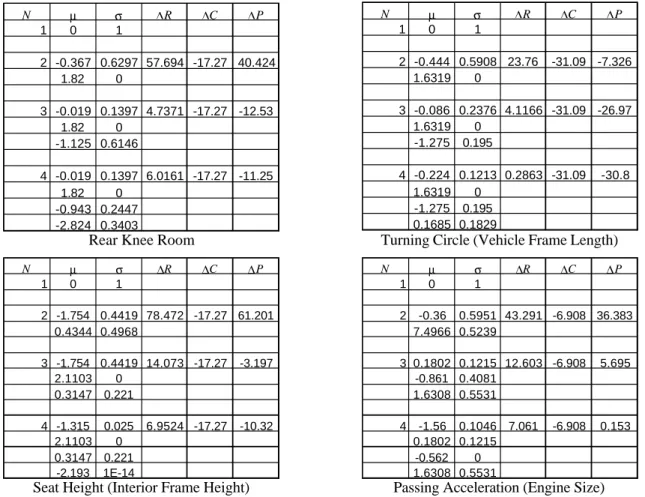
using Equation (23) to for estimated profit that can be extracted through higher pricing permitted by positioning products closer to each customer. The results for 4 attributes are shown in Figure 1, which presents relative data (means of zero and standard deviations of one on the segment statistics, and a maximum revenue of 100%). This shows that two levels of rear knee room are profitable, but three are not. Only one standard size of turning circle (vehicle wheelbase) is profitable. Two levels of seat height (body-in-white height) are profitable, and four levels of passing acceleration (engine size) are profitable. This is the main result of the analysis.
Further conclusions can be drawn from the results of Figure 1. The profitability numbers include costs, which means the recommendations consider the current development/production. One can examine the number of levels at
which each attribute begins to turn negative profit, and ask whether costs can be decreased. Areas where there are high complexity costs are particular areas of concern. For example, it would be revenue advantageous (24 revenue point increase) to offer two levels of turning circle (vehicle frame lengths), if it were not for the excessive
complexity cost to the firm. This is true as compared to, for example, three levels of seat height (14 point revenue increase) or rear knee room (5 point revenue increase). The high demand-for-variety numbers on vehicle frame length indicate that this is an area for the firm to expend R&D resources – to more easily permit multiple vehicle lengths. N µ σ ∆R ∆C ∆P 1 0 1 2 -0.367 0.6297 57.694 -17.27 40.424 1.82 0 3 -0.019 0.1397 4.7371 -17.27 -12.53 1.82 0 -1.125 0.6146 4 -0.019 0.1397 6.0161 -17.27 -11.25 1.82 0 -0.943 0.2447 -2.824 0.3403
Rear Knee Room
N µ σ ∆R ∆C ∆P 1 0 1 2 -0.444 0.5908 23.76 -31.09 -7.326 1.6319 0 3 -0.086 0.2376 4.1166 -31.09 -26.97 1.6319 0 -1.275 0.195 4 -0.224 0.1213 0.2863 -31.09 -30.8 1.6319 0 -1.275 0.195 0.1685 0.1829
Turning Circle (Vehicle Frame Length)
N µ σ ∆R ∆C ∆P 1 0 1 2 -1.754 0.4419 78.472 -17.27 61.201 0.4344 0.4968 3 -1.754 0.4419 14.073 -17.27 -3.197 2.1103 0 0.3147 0.221 4 -1.315 0.025 6.9524 -17.27 -10.32 2.1103 0 0.3147 0.221 -2.193 1E-14
Seat Height (Interior Frame Height)
N µ σ ∆R ∆C ∆P 1 0 1 2 -0.36 0.5951 43.291 -6.908 36.383 7.4966 0.5239 3 0.1802 0.1215 12.603 -6.908 5.695 -0.861 0.4081 1.6308 0.5531 4 -1.56 0.1046 7.061 -6.908 0.153 0.1802 0.1215 -0.562 0 1.6308 0.5531
Passing Acceleration (Engine Size)
Figure 1: Profitability from offering different levels on attributes. N is the number of levels, µ is the relative target for the segment, σ is the segment standard deviation of a customer when buying that target, ∆R is the lost revenue
due to not getting a higher price, ∆C is the cost in offering added levels, and ∆P is the added profit.
The next step is to determine a set of offerings to construct out of the number of levels selected on each attribute. Clustering the current SUVs using all of their attributes, we determined SUV targets for various numbers of SUVs in the family. Then, we determined which combination of levels was closest to each cluster mean. This determined the family of SUVs to offer, as well as their design attribute targets from the maximally profitable set available.
Conclusions
This paper presented an approach to determine the proper number of levels required on independent product architectural attributes, given their ability to generate added revenue through more direct targeting to smaller segments, and given the added costs of doing so. This was done in a readily implementable manner, making use only of conjoint data and cost estimates. For any selected set of attribute levels to offer, from the permutations the most effective product family using those levels can then be determined.
Acknowledgements
The research reported in this document was made possible in part by the MIT Center for Innovation in Product Development under NSF Cooperative Agreement Number EEC-9529140. Any opinions, findings, or
recommendations are those of the authors and do not necessarily reflect the views of the sponsors.
References
Ben Akiva, M. and S. Lerman, (1997) Discrete Choice Analysis, MIT Press, Cambridge, 1997.
Erens, F. J. and Verhulst, K. (1996). “Architectures for product families,” WDK workshop on Product Structuring, Delft University of Technology.
Fujita, K., Sakaguchi, H. and Akagi, S. (1999). “Product Variety Deployment and its Optimization under Modular Architecture and Module Commonalization,” 1999 ASME Design Engineering Technical Conferences, Las Vegas, Nevada. DFM-8923.
Gonzalez-Zugasti, J. P., Otto, K. N. and Baker, J. D. (1998). “A Method for Architecting Product Platforms with an Application to the Design of Interplanetary Spacecraft,” ASME Design Engineering Technical Conferences, Atlanta, Georgia. DAC-5608.
Henderson, R. M. and Clark, K. B. (1990). “Architectural Innovation: The Reconfiguration of Existing Product Technologies and the Failure of Established Firms.” Administrative Science Quarterly 35.
Jaime, M. Product Line Streamlining: A Methodology to Guide Product Costing and Decision Making, M.S. Thesis, Massachusetts Institute of Technology, 1998.
Kota, S. and Sethuraman, K. (1998). “Managing Variety in Product Families through Design for Commonality,”
ASME Design Engineering Technical Conferences, Atlanta, Georgia. DTM-5651.
Krishnan, V., Singh, R. and Tirupati, D. (1998). “A Model-Based Approach for Planning and Developing A Family of Technology-Based Products,” Austin, The University of Texas at Austin Management Department. April 1998. Working Paper.
Martin, M. and Ishii, K. (1997). “Design for Variety: Development of Complexity Indices and Design Charts,”
ASME Design Engineering Technical Conferences, Sacramento, California. DFM-4359.
Meyer, M. H. and Lehnerd, A. P. (1997). The Power of Product Platforms . New York, The Free Press.
Moore, W., Louviere, J. and R. Verma, (1998). “Using Conjoint Analysis to Help Design Platforms,” Marketing Science Institute, Journal of Product Innovation Management, 16(1):27–39.
Mosher, R. The Use of a Product End of Life Process to Effectively Manage a Product Portfolio, M.S. Thesis, Massachusetts Institute of Technology, 1999.
Nelson, S., Parkinson, M. and P. Papalambros, (1999). “Multicriteria Optimization in Product Platform Design,”
ASME Design Engineering Technical Conferences, Las Vegas, Nevada. DAC-8676.
Pedersen, P. (1999). “Organisational Impacts of Platform Based Product Development.” International Conference on
Engineering Design, Munich.
Pulkkinen, A., Lehtonen, T. and Riitahuhta, A. (1999). “Design for Configuration - Methodology for Product Family Development,” International Conference on Engineering Design, Munich.
Roberson, J. Designing Effective Portfolio Variety Using Customer Need Discrimination Thresholds, M.S. Thesis, Massachusetts Institute of Technology, 1999.
Robertson, D. and Ulrich, K. (1998). “Planning for product platforms,” Sloan Management Review 39(4):19-31. Sanderson and Uzumeri (1995). “Managing Product Families: The Case of the Sony Walkman,” Research Policy,
24:761-782.
Sawtooth Technologies, Inc. (2000). http://www.sawtooth.com/.
Urban, G. and J. Hauser, (1993). Design and Marketing of New Products. Prentice Hall, 2nd edition, New York. Weir, O. Analysis of Customer-Driven and Systemic Variation in the Airplane Assembly Process, M.S. Thesis,
Massachusetts Institute of Technology, 2000.
Wheelwright, S. and K. Clark, (1992). “Creating Project Plans to Focus Product Development.” Harvard Business
Review, March-April.