Airline O-D control using network displacement concepts

(1)

r

I 2'J~)

FLIGHT TRANSPORTATION LABORATORY REPORT R97-1

AIRLINE O-D CONTROL USING NETWORK DISPLACEMENT CONCEPTS

(2)

(3)

1

Introduction ...- --.--- 11

1.1 M otivation for Revenue M anagem ent... 11

1.2 G oal of The Thesis... 14

1.3 Structure of The Thesis... 15

2 Existing Revenue M anagem ent M ethods... 16

2.0 Introduction... 16

2.0.1 Partitioned Network Optim ization... 16

2.0.2 Heuristic Nesting M ethod... 18

2.0.3 Some Issues... 19

2.1 Leg Based Fare Class YM ... 19

2.1.1 Process of the M ethod... 21

2.1.2 Sum m ary... 23

2.2 Greedy Nesting... 23

2.2.1 Fare Stratification... 24

2.2.2 Greedy Virtual Nesting...24

2.2.3 Sum m ary... 26

2.3 EM SR Heuristic Bid Price... . 26

2.3.2 Sum m ary...30

2.4 Non-greedy Virtual Nesting... 30

2.4.2 Sum m ary... 35

2.5 Network Determ inistic Bid Price... 35

2.5.2 Summ ary... 36

2.6 Chapter Summary... 37

3 Approaches to Network O-D Control Considering Displacement Im pacts... 39

3.1 Non-greedy Heuristic Bid Price Control M odel... 39

3.1.1 Introduction... 39

3.1.2 The M odel... 40

3.1.3 Some Concerns about the Non-greedy Heuristic Bid Price M odel ... 45

3.2 Convergent EM SR Control M odel... 56

3.2.1 Introduction... ... 56

3.2.2 An Observation... 56

3.2.3 The M odel... 57

(5)

4 Case Studies... 60

4.1 The Booking Process Simulation... 60

4.2 Network Characters... 63

4.3 Strategy Comparison... 65

4.3.1 Leg Based Fare Class Yield Management (LBFC)...65

4.3.2 Greedy Virtual Nesting (GVN)... 70

43.3 Greedy Heuristic Bid price(GHBP)... 75

4.3.4 Non-greedy Virtual nesting (NGVN)... 78

4.3.5 Deterministic Network Bid Price (DNBP)... 83

4.3.6 New Methods...84

4.4 Conclusions... 111

5 Conclusions... 116

Appendix 1 Calculation of EM SR Curve...121

2 LP Solution Output File... 131

3 Shadow Prices Comparison...133

4 Comparison between Shadow Prices and Critical EMSR Values... 134

5 Comparison between Shadow Prices, EMSR Values, and Converged EMSR Values... 136

(6)

List of Figures

1.1 Single Fare Product Example... . ... 11

1.2 M ultiple Fare Product Exam ple... 12

1.3 Booking Performance of Different Fare Types before Departure... 13

2.1 A Sim ple Network with 2 Legs... 20

2.2 EMSR Curve from Greedy Virtual Nesting Method on Leg 1... 27

2.3 EMSR Curve from Greedy Virtual Nesting Method on Leg 2... 28

2.4 EMSR Curve Based on Pseudo Fares on Leg 1...33

2 EMSR Curve Based on Pseudo Fares on Leg 2...34

3.1 A Tw o-Leg N etw ork...48

3.2 Process of the Non-greedy Seat Controls Method...52

3.3 Revised Process of the Non-greedy Seat Inventory Control Method... 53

3.4 Distribution of the Shadow Prices... 54

3.5 A Two-leg Segment Network... 57

3.6 Convergence in Fare Distribution... 58

4.1 Tim e Line of the Sim ulation... 62

4.2 Sim ulation Process... 63

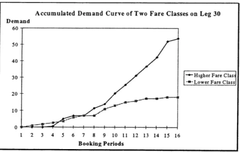
4.3 Demand Curve for Two Fare Classes on Leg 30... 64

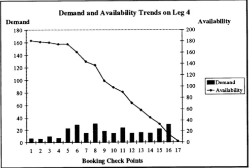
4.4 Mean Demand and Availability Trends Over 18 Booking Periods on Leg 4...67

4.5 Spill Performance for Fare Class 3 on Leg 30...69

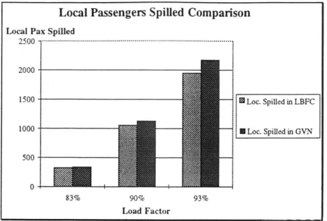
4.6 Comparison of Number of Local Passengers Spilled...72

4.7 Comparison of Number of Connecting Passengers Spilled...72

4.8 Availability Comparison between LBFC and GVN on Leg 4...74

4.9 Availability Comparison between LBFC and GVN on Leg 30... 74

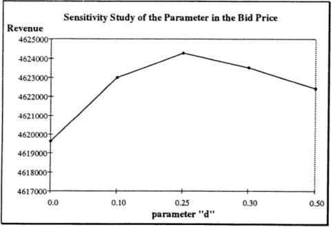
4.10 Sensitivity Studies of Bid Price Formula for GHBP Method...76

4.11 Process Comparison between the GVN and the NGVN...79

4.12 Revenue/Passenger Comparison between GVN and NGVN at D em and Level 1.20... 81

4.13 Revenue/Seat Comparison between GVN and NGVN at D em and Level 1.20... 82

4.14 Process of the DNBP M ethod... 83

4.15 Process of the NGHBP M ethod... 85

4.16 Comparison in Revenue/Passenger between GHBP and NGHBP Methods...87

4.17 Comparison in Revenue/Seat between GHBP and NGHBP Methods... 87

4.18 Sensitivity Studies of Parameter in Bid Price Formula for NGHBP Method...89

4.19 Comparisons of Percentage of Spills between GHBP and NGHBP at D em and Level 1.20... 90

4.20 Availability Comparison between GHBP and NGHBP on Leg 4... 91

(7)

List of Tables

2.1 Fare and Demand Information on Leg 1...20

2.2 Fare and Demand Information on Leg 2...20

2.3 Fare Groups in Leg Based Fare Class YM Method... 21

2.4 Demand-weighted Mean Fare for EMSR Input... 22

2.5 Seats Protection using Fare Class Nesting...22

2.6 Booking Limits in Leg Based Fare Class YM Method...23

2.7 Fare Groups in Fare Stratification... 24

2.8 V irtual Classes on Leg 1... 25

2.9 V irtual Classes on Leg 2... 25

2.10 Seats Protection using Virtual Class Nesting... 25

2.11 Booking Limits in Greedy Virtual Nesting Method... 26

2.12 EM SR Heuristic Bid Prices... 29

2.13 Booking Decisions for Local Passengers on Leg 1... 29

2.15 Booking Decisions for Connecting Passengers... 29

2.16 Pseudo Fares of Connecting Passengers... 32

2.17 Virtual Classes based on Pseudo Fares on Leg 1... 32

2.18 Virtual Classes based on Pseudo Fares on Leg 2... 33

2.19 Seats Protection in Non-greedy Virtual Nesting Method... 34

2.20 Booking Limits in Non-greedy Virtual Nesting Method... 34

3.1 EMSR Heuristic Bid Prices Based on Pseudo Fares... 42

3.5 Pseudo Fares of Connecting Passengers...43

3.6 EMSR Heuristic Bid Prices Based on Pseudo Fares... 43

4.1 D em and Scenarios... 64

4.2 Network Performance of LBFC Method using EMSRa Control...66

4.3 Network Performance of LBFC Method using EMSRb Control...66

4.4 Performance of LBFC method on Two Selected Legs at Demand Level 1.20..67

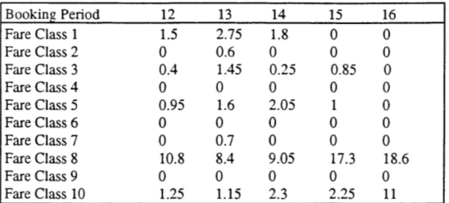
4.5 Demands come During the Last 5 Booking Periods on Leg 4...68

4.6 Booking Performance During the Last 5 Booking Periods on Leg 4...68

(8)

4.22 Comparisons of Percentage of Spills between NGVN and NGHBP at

D em and Level 1.20... 93

4.23 Comparisons of Percentage of Spills between NGVN and NGHBP at D em and Level 0.80... 93

4.24 Running LP at Different Demand Levels (NGVN Method)... 95

4.25 Running LP at Different Demand Levels (NGHBP Method)... 96

4.26 Multiple LP vs. Single LP... 97

4.27 Sensitivity Study for LNGBP at Demand Level 1.20... 102

4.28 A Loop to Find the Converged Pseudo Fares Based on C ritical EM SR V alues... 104

4.29 Sensitivity Studies in CONPSF at Demand Level 1.20... 107

4.30 Convergence Process of Prorating a 2-Leg Fare (O-D Pair 7, Class 1) using H alf F are to Start... 108

4.31 Converge Process of Prorating a 2-Leg Fare (O-D Pair 7, Class 1) using T otal F are to Start... 109

4.32 M ethod C om parison... 112

4.33 Method Comparison in Another Network ... 113

(9)

4.8 Ranges of 10 Virtual Classes on Leg 4 and Leg 30 in GVN Method... 70

4.9 Perform ance of GVN M ethod... 71

4.10 Performance of GVN on Two Selected Legs at Demand Level 1.20... 73

4.11 GHBP Control Applied to Only Connecting Passengers... 75

4.12 GHBP Control Applied to Both Connecting and Local Passengers... 75

4.13 Comparison between the GVN and the GHBP Methods... 77

4.14 Leg Performance of the GHBP at Demand Level 1.20... 77

4.15 Comparison between the GVN and the GHBP on Leg 4... 77

4.16 Average Spill comparison Between GVN and GHBP by Virtual Classes... 78

4.17 16 Virtual Class Ranges on Leg 4 and Leg 30 in NGVN Method...79

4.18 Revenue Performance of the NGVN Method... 80

4.19 Comparison between GVN and NGVN at Demand Level 1.20... 80

4.20 Comparison between GVN and NGVN at Demand Level 0.80... 80

4.21 Leg Perform ance of NGVN ... ... 82

4.22 Comparison of GVN and NGVN on Leg 4... 82

4.23 Network Performance of DNBP... 84

4.24 Revenue Performance of the NGHBP Method... ... 85

4.25 Revenue Performance of the NGHBP Method with fixed Parameter at 0.50...86

4.26 Comparison of Network Performance Between GHBP and NGHBP at D em and Level 1.20... 86

4.27 Comparison of Network Performance Between GHBP and NGHBP at D em and Level 0.80... 86

4.28 Seat Control Performance of NGHBP Method on Leg 4 and Leg 30...88

4.29 Comparison of Seat Controls between GHBP and NGHBP m ethods on Leg 4... 88

4.30 Network Performance Comparison between NGVN and NGHBP at D em and Level 1.20... 92

4.31 Network Performance Comparison between NGVN and NGHBP at D em and Level 0.80... 92

4.32 Comparison between NGVN and NGHBP on Leg 4... 92

4.33 Comparison between NGVN and NGHBP on Leg 30... 93

4.34 Shadow Price Studies... 98

4.35 Revenue Performance of the LNGBP method... 99

4.36 Leg Performance of the LNGBP Method...99

4.37 Comparison between the Shadow Prices and the Critical EMSR Values... 100

4.38 Comparison of Virtual Class Ranges between NGHBP and L N G B P on L eg 4... 101

4.39 Comparison of Virtual Class Ranges between NGHBP and LN G B P on Leg 30... 101

4.40 Comparison of Network Performance Between NGHBP and LNGBP at D em and Level 1.20... 101

4.41 Comparison of Network Performance Between NGHBP and LNGBP at D em and Level 0.80... 102

4.42 Comparison of Network Performance Between GHBP and LNGBP at D em and Level 1.20... 103

(10)

4.43 Comparison of Network Performance Between GHBP and LNGBP

at D em and Level 0.80... 103

4.44 Revenue Performance of the Revised LNGBP Method... 104

4.45 Comparison of Virtual Class Ranges among NGHBP, LNGBP, and C O N PSF on L eg 4... 105

4.46 Comparison of Virtual Class Ranges among NGHBP, LNGBP, and C O N PSF on Leg 30... 105

4.47 Revenue Performance of the CONPSF Method...106

4.48 Leg Performance of the CONPSF Method... 106

4.49 Comparison of Network Performance Between LNGBP and CONPSF at Dem and Level 1.20... 106

4.50 Comparison of Network Performance Between LNGBP and CONPSF at Dem and Level 0.80... 106

4.51 Comparison of NetworkPerformance Between NGHBP and CONPSF at Dem and Level 1.20... 107

4.52 Comparison of Network Performance Between NGHBP and CON PSF at D em and Level 0.80... 107

4.53 Revenue Performance of the Connecting Fare Proration Convergence M eth od ... 109

4.54 Leg Performance of the Connecting Fare Proration Convergence M eth od ... 109

4.55 Comparison between the CONPRT methods with Different Starting Points.... 110

4.56 Network Performance Comparison Between the CONPSF and the CONPRT methods at Demand Level 1.20... 110

4.57 Network Performance Comparison Between CONPSF and CONPRT at D em and L evel 0.80... 110

4.58 Network Performance Comparison Between NGHBP and CONPRT at D em and Level 1.20... 111

4.59 Network Performance Comparison Between NGHBP and CONPRT at D em and L evel 0.80... 111

4.60 D em and Scenarios... 113

4.61 Upper Bound for the Sm aller Network... 115

(11)

Chapter 1 Introduction

1.1 Motivation for Revenue Management

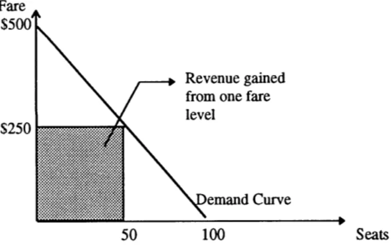
Revenue Management is an attempt by airlines to optimize their total revenue by achieving a different passenger mix on each flight departure for those passengers paying full fares, those paying discount fares, and those paying deep discount fares'. It includes two processes: Price Differentiation and Seat Inventory Control. In the pricing differentiation process, airlines try to distribute passengers into different groups and make the passengers who are able to pay more spend as much as they can, and make the remaining seats, which otherwise will be empty, available for those passengers who will not travel if the price is too high. Figure 1.1 is a demand curve of a particular flight. We know that the optimal

potential revenue from this flight is the whole area under the demand curve, which is

$25,000.

Revenue gained from one fare level

Curve

50 100 Seats

Figure 1.1 Single Fare Product Example

GAOIRCED-90-102, Fares and Service at Major Airports

Fare $500

(12)

If a single fare level strategy is employed, the revenue the airline can achieve from this flight is only $12,500 (the shaded area). In practice, sometimes, a single fare level will not cover total operating costs2_{. However, under the same demand assumption, if the airline}

offers seats at three different fare levels and if we assume there are perfect strategies to segment the passengers, then the total revenue the airline can acquire will be $18,750. Figure 1.2 explains how those three fare levels can provide a higher total network revenue than the single fare strategy.

Fare $500

Revenue gained from three fare levels

$125

Demand Curve

25 50 75 100 Seats

Figure 1.2 Multiple Fare Product Example

Such a fare structure increases the total revenue and makes it easier for an airline to cover total operating costs.

As Williamson (1992) wrote in her thesis "the airlines are not directly discriminating in price between different passengers for the same fare product. The differential in price offered by airlines is usually based on differences in fare products, each of which is uniquely defined by restrictions on their purchase and use for air travel." In order to obtain the benefits of price differentiation, the airlines must manage their fare levels and the restrictions associated with those fare levels effectively.

In practice, several issues need to be considered to achieve revenue maximization. First, how many fare levels should an airline set in its fare structure? Theoretically, there should be as many fare levels as the number of seats on each flight, which means one price for each passenger. One obvious problem of this scheme is that the complicated fare structure will confuse not only the passengers but also the travel agents. It is also difficult to

employ this theory in the real world due to a lack of perfect information about the price 2 E.L.Williamson, Airline Network Seat Inventory Control: Methodologies and Revenue Impacts, Flight Transportation Lab Report, R92-3, June 1992.

(13)

elasticity for every single passenger. Furthermore, as the number of the different fare prices increases, the cost for advertisement and reservation systems will increase.

Considering all those elements, most airlines have no more than 10 different fare products for each market.

Second, how should the airlines prevent the time sensitive business passengers from taking advantage of certain low fare products designed for the price sensitive leisure passengers? Usually, the airlines place some restrictions along with each discounted fare product, such

as Saturday night stay, 7/14 days advance purchase, etc. In practice, these restrictions are, at least as, if not more, important than how many fare levels the airlines should offer.

The third issue relating to revenue maximization regards the booking strategy. Usually in the real world operation, the low fare passengers are more likely to request bookings earlier, while the full fare passengers tend to come late and book at the last minute before a flight. Figure 1.3 shows hypothetical booking curves of different fare types.

Passengers _Deeply

Discounted Fare

Full Fare

5b4b 3 b 2 b l

Days Prior to Departure

Figure 1.3 Booking Performance of Different Fare Types before Departure

From the figure above we can see that the deep discount requests come much earlier than full fare requests. The airlines then face a trade-off as to whether they should give a seat to a low fare passenger or reserve it for a last minute high fare passenger, but if he/she does not materialize then this seat will go empty. Therefore, it is very important for an airline to control the number of seats available as discounted fare products and to reserve enough seats for last minute high fare passengers. This process is called seat inventory control. It is an attempt for airlines to balance the number of seats sold at each fare level

(14)

so as to maximize total passenger revenue. Belobaba(1987) said in his doctoral thesis, "The seat inventory control process is a tactical component of revenue management that is entirely under the control of each individual airline and is hidden from consumers and competitors alike.... Nevertheless, seat inventory control has the potential of increasing total revenues expected from flights on a departure-by-departure basis, something that would be far more difficult through pricing actions."3

1.2 Goal of The Thesis

In the competition among airlines, price differences are no longer determined by how low an airline's fare levels are. If we look at the published fare prices of the airlines in

America, most airlines have the same fare prices. The primary difference among them is how many seats are available to each fare product by each airline on each flight it operates.

Generally speaking, there are five major different seat inventory control methods applied or being developed in the airline industry today.

" Leg Based Fare Class Yield Management.

" Greedy Virtual Nesting and/or Fare Stratification Yield Management. * Greedy EMSR Heuristic Bid Price.

" Non-greedy Virtual Nesting based on Network Displacement. " Network Bid Price Control.

One objective of this thesis is to analyze the algorithms of these five methods, see how they are applied in the real world, and identify the major differences among them. Then, a new revenue management method is proposed. This method combines the merits of both the EMSR Heuristic Bid Price method and the non-greedy virtual nesting method, and it shows revenue improvement with the true data from several airlines.

' P.P. Belobaba, Air Travel Demand And Airline Seat Inventory Management, Flight Transportation Laboratory Report, R87-7, May 1987.

(15)

1.3 Structure of the Thesis

This thesis includes five chapters.

Following this introductory chapter, in Chapter 2, the five existing major yield management methods will be briefly discussed. Using a simple example, the major differences among these five methods will be considered, and pros and cons associated with each method will be addressed.

In Chapter 3, a new revenue management method is proposed. In this new method, we will employ network optimization tools to obtain the displacement impact of the

connecting passengers. Then, passengers are booked based on the consideration of their whole network revenue contribution. Several implementation issues associated with this new method are also discussed.

In Chapter 4, actual data from two airlines will be used to compare the different revenue performance of these six revenue management methods through simulation. For the new proposed method, sensitivity analyses will be presented to identify the best formula in the bid price calculation.

(16)

Chapter 2 Existing Revenue Management Methods

As a prelude to the extension of existing models in the subsequent chapter, this chapter presents an overview of the mathematical approaches developed previously. There are

-five major methods introduced here: Leg Based Fare Class Yield Management, Greedy Virtual Nesting, Heuristic Bid Price, Non-greedy Virtual Nesting, and Network Bid Price. A simple example will be used to explain these methods. Also, the booking limits

calculated from these five different methods are compared.

2.0 Introduction

Generally speaking, the approaches to seat inventory control can be divided into two major groups, the partitioned network method and the heuristic nesting method. In a partition method, the solution is simply the number of seats allocated to each origin-destination (OD) fare product, while in a heuristic nesting method the solution is the number of seats protected for a group of OD fare products.

2.0.1 Partitioned Network Optimization

One way to solve the seat inventory control problem is by using network optimization tools to solve the following linear program (LP) problem':

1 B. L. Williamson, Airline Network Seat Inventory Control: Methodologies And Revenue Impacts, Flight

(17)

Max:

ODs FareClasses

Re venue = 2 fare(i, j)x(i, j); [2.1]

i J

Subject to:

x(ij)eLeg(k)

x(i, j) Capacity(k) , for all leg k;

i~j

x(i,j) Demand (i, j), for all OD pairs;

where in the formula, i is the number of the OD pairs, and

j

is the fare class number. This is a partitioned method because the x(ij) is simply the allocation of seats to each OD fare. Once a seat is allocated to an OD fare, it can only be used by that OD fare. The limitation of this method is that it ignores the stochastic chara-ter of demand because, in the second set of constraints, the right hand side Demand(ij) is just tie mean of each OD demand. So this method assumes perfect demand forecasting and zero demand deviation.

One more drawback of this method is that it is difficult for an airline to collect the data on demand for all OD fares in a large network. Most computer reservation systems do not routinely store information to support such a network optimization process. In the

meantime, since the data changes with the booking periods, how often an airline should re-run such a large optimization process becomes critical. Re-re-running this process too

infrequently will make a negative network revenue impact while re-running it too often is very uneconomical.

Another shortcoming of this method is the "small numbers" problem. For a hub network with 25 flights in and 25 flights out of a connecting hub, there can be 26 different OD itineraries on a single flight leg. With 10 fare classes and an overall average aircraft size of

158 seats2_{, the number of seats per}_OD_{fare is, on average, less than}_13. _{In addition, there}

will be a great chance that a seat remains empty due to the deviation of demand. These

4

reasons make such partitioned network optimization rarely used in the airline industry .

2 Airline Economics, Inc., Datagram: _{Major U. S. Airline Performance,}_{Aviation Week & Space}

Technology, Volume 133, October 8, 1990.

3 B. L. Williamson, Airline Network Seat Inventory Control: Methodologies And Revenue Impacts, Flight Transportation Laboratory Report, R92-3, June 1992.

4 P.P. Belobaba, Airline O-D Seat Inventory Control Without Network optimization, Flight Transportation Laboratory, June 1995.

(18)

2.0.2 Heuristic Nesting Method

The airline seat inventory management problem is probabilistic because there exists

uncertainty about the ultimate number of requests that an airline will receive for seats on a future flight and, more specifically, for the different fare classes offered on that flight5. Nested Heuristics is different from the partitioned method in that it divides all the network OD fares into several groups. Seats are thereby allocated to each group. It is like

protecting seats for higher fare products from lower ones. In his doctoral thesis,

Belobaba6 presented a heuristic nesting method called Expected Marginal Seat Revenue (EMSR) method to solve the multiple fare class problem on a single leg. In this method, Belobaba proposed using the expected marginal seat revenue to determine the number of seats that should be protected for each higher fare class i over the lower fare class

j.

By the definition of this method, the seat will be protected for the higher fare class as long as the following equatio, Wodc

EMSR(S') = Farei x FP(S) > Fare1 [2.2]

where i is the higher fare class, while

j

is the lower fare class. Then, the seat protection for the highest fare class H1 is simply S . However, the number of seats that should be

1 2

protected for the two highest fare classes, H2, is defined as the sum of S3 and S3 determined separately from the equation above. Therefore the booking limits, BLi, the

number of seats available to each fare class, is defined as the capacity minus the number of seats protected for all higher fare classes.

BLi = Capacity - H i-_ [2.3]

This method is known as EMSRa. In 1992, Belobaba suggested another method known as EMSRb. In this method, he proposed to calculate the seat protection levels jointly for all higher fare classes relative to a given lower class, based on a combined demand

forecast and a weighted price level for all classes above the one for which a booking limit is being calculated. The weighting is done based on expected demand that class7_{. Such}

5 P.P. Belobaba, Air Travel Demand and Airline Seat Inventory Control Management, Flight Transportation Laboratory Report, R87-7, May 1987.

6 P.P. Belobaba, Air Travel Demand and Airline Seat Inventory Control Management, Flight

Transportation Laboratory Report, R87-7, May 1987.

7 P.P. Belobaba, Comparing Decision Rules that Incorporate Customer Diversion in Perishable Asset

(19)

method has been shown to have higher net revenue in practice of seat inventory control than the partitioned network method.

2.0.3 Some Issues

Before we do any research, we must understand what makes a revenue management method implementable in the airline industry. First, of course, there must be network revenue improvement. Second, which is very important yet easy to ignore, is that the information to support the method must be easy to access. That is why some of the methods we discuss in this chapter cannot be implemented in the real world even though they give very good revenue performance.

Following we will discuss five different revenue management methods that are implemented or being developed in the airline industry in order to find out why some methods perform better than others. Such information provides a direction for our research.

2.1 Leg Based Fare Class YM

In this method, data are collected based on each leg and fare class, and forecasts are made based on each leg. All OD fares that traverse the same legs are divided into several fare groups based on their relative yield and restriction types no matter whether they are local fares or connecting fares. Next, the EMSRb method is used to calculate the number of seats that should be protected for each group of fare products. The fare value, which represents each fare group, used as the input for the EMSRb calculation, could be demand-weighted-mean fares, local fares, or prorated fares.

The following example will be helpful to explain this method. Figure 2.1 shows a very simple network with only two legs.

(20)

0

A

leg0 leg 2

-Figure 2.1 A Simple Network with 2 Legs

Suppose we have the following information about the demand and fares.

Leg 1: 500 miles in trip length.

Fare Class Fare Demand Standard Deviation

Local Passengers Y 500 10 5 B 300 20 8 Q 150 40 15 Connecting Passengers Y 1000 8 4 B 625 25 10 Q 250 45 17

Table 2.1 Fare and Demand Information on Leg 1

Leg 2: 600 miles in trip length.

Fare Class Fare Demand Standard Deviation

Local Passengers Y 600 15 6 B 350 25 10 Q 200 45 17 Connecting Passengers Y 1000 8 4 B 625 25 10 Q 250 45 17

Table 2.2 Fare and Demand Information on Leg 2

There are three steps to fulfill the inventory control process: grouping fares, generating EMSR inputs, and calculating booking limits.

(21)

2.1.1 Process of the Method

1. Grouping of the Fares

The leg-based fare class yield management is a nesting heuristic method, and it involves nesting by fare class. In this method, the fares are grouped into different classes based on their fare classes. In our example here, there are three fare classes, full fare Y class, business B class, and discount

Q

class. All OD fares that cross one particular leg will be grouped in a class, which is the same as their fare classes, no matter whether they are local fares or connecting fares. Therefore we will have the following fare groups:

Leg 1 Leg 2

Y classes: Y(AB) Y(AC) Y classes: Y(BC) Y(AC)

B classes: B(AB) B(AC) B classes: B(BC) B(AC)

Q

classes: Q(AB) Q(AC) Q classes: Q(BC) Q(AC)

Table 2.3 Fare Groups in Leg Based Fare Class YM Method

The seats will be protected according to each of those groups.

2. EMSR Fare Inputs

The fares in each fare group are not the same. For example, fares in Y class on leg 1 are

FareY(AB) = $500, and

FareY(AC) = $1000.

[2.4]

Therefore, before calculating the EMSR curve, we need to decide which value of a fare should be used as EMSR input. There are several ways to decide this8: Demand Weighted Mean Fare, Local Fare, Mileage Prorated Fare, and Local Fare Prorated Fare. In this thesis, we will use the demand weighted fare as our input.

8 E.L. Williamson, Airline Network Seat Inventory Control: Methodologies And Revenue Impacts, Flight Transportation Laboratory Report, R92-3, June 1992.

(22)

. Demand Weighted Mean Fare

In this method, the fares are weighted by demand. In our example, for instance, Y class on leg 1, the demand-weighted fare can be calculated as follows:

Fare = Fare(AB) x Demand(AB) + Fare(AC) x Demand(AC) Demand(AB) + Demand(AC)

= $722.22

In the same way, we can obtain other input fares as shown in Table 2.4.

Y class B class Q class

Leg 1 $722.22 $462.50 $225.00

Leg 2 $739.13 $480.56 $202.94

Table 2.4

[2.5]

Demand-weighted Mean Fare for EMSR Input

3. Calculating the EMSR Seat Protection for Each Fare Group

The rule of EMSR seat protection is: as long as the Expected Marginal Seat Revenue of the higher fare class is higher than the next lower fare class, the seats should be protected for the higher fare class passengers. The formula for such protection is given in (2.2). From this formula, we can calculate the number of seats that should be protected for each fare level. In this calculation, EMSRb method is implemented to decide the protection. Please refer to Belobaba (1992) for a detailed description. The solutions are listed in the following table.

Seats Protection using Fare Class Nesting Y class Y and B classes Seats Protection on Leg 1 16 66 Seats Protection on Leg 2 20 78

(23)

Using formula (2.3) we have the following booking limits for each class:

Y class B class Q class

Booking Limits on Leg 1 100 74 34

Booking Limits on Leg 2 100 80 22

Table 2.6 Booking Limits in Leg Based Fare Class YM Method

For local passengers, if the booking limits of their corresponding fare classes are greater than zero, then they are booked. On the other hand, the connecting passengers can be booked if and only if the booking limits of their fare classes are greater than zero on all the legs they traverse.

2.1.2 Summary

This method directly uses the fare classes to group the fares regardless of whether they are local fares or connecting fares. Hence it is easy to implement and normally results in a passenger mix with a high yield. However, this method tends to give priority to short haul high yield passengers; therefore it may take the risk of spilling lower yield but high revenue long haul connecting passengers. This may cause a negative network revenue impact especially when demand is low and there are empty seats remaining on some legs. Under such a circumstance, taking one connecting passenger from a lower fare class may produce more network revenue contribution than one local passenger from a higher fare class.

2.2 Greedy Nesting

First proposed by Boeing9, in this method, OD fares are assigned to different inventory buckets according to a fare range associated with the bucket. OD fares within each

bucket are then controlled as a group. "Greedy" here means the nesting approach is based totally on the itinerary fare value, and it will tend to give higher priority to long haul, 9_{Boeing Commercial Airplane Company, A Pilot Study of Seat Inventory Management for a Flight}

(24)

connecting passengers. This method can be divided into two different sub-methods: Fare Stratification and Virtual Nesting. They are similar since both of them are "greedy", while they differ in the way they are implemented.

2.2.1 Fare Stratification

This method is distinguished from Fare Class Nesting because it groups all fares on each leg into several classes based on their fare values. The number of those classes is generally the same as the number of the fare classes, but used in a separate way. For example, determined by the number of booking classes in the system, we can choose to cluster the fares into four groups as follows (based on their total fare value):

Leg 1 Leg 2

Y class Y(AC) Y class Y(AC)

B class Y(AB), B(AC) B class Y(AB), B(AC)

Q class B(AB), Q(AC) Q class B(AB), Q(AC)

V class Q(AB) V class Q(AB)

Table 2.7 Fare Groups in the Fare Stratification Method

Next, we use demand-weighted mean fare or mileage-weighted mean fare to calculate the EMSR input, then calculate the seat protection for each fare class group. Since, in this method, we have put the full fare connecting passengers in the highest fare class, they will have the higher priority to access the seats than full fare local passengers. The local discount fare, which has the lowest fare value, is ranked in V class, and it will be the first class to be rejected (spilled) if the demands exceed the seat capacity.

2.2.2 Greedy Virtual Nesting

In contrast to Fare Stratification, in this method, the fares are no longer assigned to Y, B,

Q

and V classes. Instead, they are grouped into several so-called "virtual" classes by their fare values. The number of virtual classes can be arbitrarily selected. The maximum number of virtual classes can be equal to the number of different fare values on each leg. Following are the virtual classes for our example in Figure 2.1.

(25)

Leg 1:

Leg 2:

Virtual Classes Fare Classes Fare

Y1 Y(AC) $1000 Y2 B(AC) $625 Y3 Y(AB) $500 Y4 B(AB) $300 Y5 Q(AC) $250 Y6 Q(AB) $150

Table 2.8 Virtual Classes on Leg 1

Virtual Classes Fare Classes Fare

Y1 Y(AC) $1000 Y2 B(AC) $625 Y3 Y(BC) $600 Y4 B(BC) $350 Y5 Q(AC) $250 Y6 Q(BC) $200

Table 2.9 Virtual Classes on Leg 2

Here we have chosen an extreme case, where each fare value is in a different virtual class, and the fares are ranked totally based on their itinerary fares. Next, based on these virtual classes, the EMSR value will be calculated. The calculation is exactly the same as what has been done in leg-based fare class yield management method. The seat protection and booking limits are given in the following tables. For the detailed calculations, please refer to Appendix 1.

Y1 Y2 Y3 Y4 Y5

Seats Protection on Leg 1 7 27 44 65 116

Seats Protection on Leg 2 7 22 48 75 121

Table 2.10 Seats Protection using Virtual Class Nesting

(26)

Y1 Y2 Y3 Y4 Y5 Y6

Booking Limits on Leg 1 100 93 73 56 35 0

Booking Limits on Leg 2 100 93 78 52 25 0

Table 2.11 Booking Limits in the Greedy Virtual Nesting Method

Comparing the results in Tables 2.10 and 2.11 with the results given in Table 2.5 and 2.6, we can see that, unlike the leg-based yield management method, in which both local and connecting

Q

classes have seats available, the virtual class Y6, local

Q

class, is not available while virtual class Y5 (connecting

Q

class) is still available. This is due to the greedy virtual nesting method giving higher priority to the long haul high fare passengers.

2.2.3 Summary

Unlike the leg-based fare class YM method, this method groups the fares according to their total fare values, so it tends to give more favor to the high fare long haul connecting passengers. For a simple network like Figure 2.1, which has only 2 legs, there are four circumstances depending upon the demand: Both legs have low demand, both legs have high demand, Leg 1 has low demand while Leg 2 has high demand, or Leg 1 has high demand while Leg 2 has low demand. In three out of four of these cases, that is, when both legs or at least one of the legs has empty seats, such a method is desirable. However, when the demand is severely high and both legs have spill, this method may have a

consequential negative impact. This is because, under such a condition, booking two local passengers can give have higher total network revenue contribution than booking one connecting passenger.

2.3 EMSR Heuristic Bid Price

The greedy virtual nesting method groups the fares in the virtual classes based totally on their fare values. The disadvantage with such a strategy is that, when the demands on both legs are extremely high, loading one connecting passenger while spilling two local passengers, whose total fares are higher than one connecting passenger, will have a

(27)

negative network fare impact. The idea of the heuristic bid price method (Belobaba 1995) is to capture the displacement impact of a connecting passenger onto the local passengers. It uses the virtual classes to calculate the current EMSR curve, then uses this EMSR value to set a "cut-off" price called "bid price." For the local passengers, this bid price is simply the current EMSR value on that leg. For the connecting passengers, the bid price will be the combination of EMSR values on all legs the fare traverses. Next, we will use the example in Figure 2.1 to explain this method.

2.3.1 Process of the Method

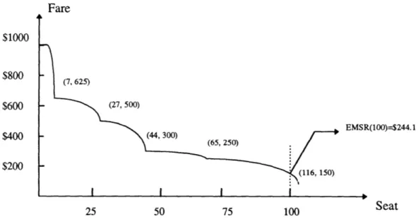
1.EMSR Curve Calculation

As shown in Table 2.8 and 2.9, we have six virtual classes on both Leg 1 and Leg 2. Suppose the capacity on each leg is 100. The EMSR curve is shown below.

$1000 $800 $600 $400 $200 Fare (7, 625) (27, 500) (44, 300) EMSR(100)=$244.1 (65, 250) 25 50 75 100

Figure 2.2 EMSR Curve from Greedy Virtual Nesting Method on Leg 1

On leg 2, we can find a similar EMSR Curve:

Seat

(28)

Fare (7, 625) (22, 600) (48, 350) (78,250) 25 50 75 100 Figure 2.3 EMSR $1000 $800 $600 $400 $200

Curve from Greedy Virtual Nesting Method on Leg 2

The detailed calculations of these two curves and the EMSR value of the 100th seat are in Appendix 1.

2. Calculation of the Bid Price

For the local fare, the bid price is simply the EMSR value on that leg. For the connecting fare, the formula of the bid price on leg 1 is given as

BP = EMSR, +d x EMSR2. [2.6]

While the bid price on leg 2 is given as

BP2 = EMSR2 +d x EMSR. [2.7]

The "d" is the product of the percentages of the local passengers on both legs, and its range is 0 <_d < 110.

On this basis, we can obtain the following bid price:

10 P.P. Belobaba, Airline O-D Seat Inventory Control Without Network Optimization, Flight Transportation Laboratory, MIT, June 1995.

0 EMSR(100)=$250

(121, 200)

(29)

Leg 1 Leg 2

Local 244.1 250

Connecting 306.6 311.0

Table 2.12 EMSR Heuristic Bid Prices

3. Booking Limits

Considering the bid prices, we can decide whether a passenger should be booked or spilled. For local passengers, if their fares are higher than the bid price on the leg they traverse, they can be booked. For connecting passengers, their fares must be higher than the bid prices on all legs they traverse. As a result, we have the following tables showing the airline's booking decision for local and connecting passengers:

Local fares on Leg 1:

Local

Fare Bid Price Book/Spill

Y3 500 244.1 Book

Y4 300 244.1 Book

Y6 150 244.1 Spill

Table 2.13 Booking Decisions for Local Passengers on Leg 1 on Leg 2:

Y3 600 250 Book

Y4 350 250 Book

Y6 200 250 Spill

Table 2.14 Booking Decisions for Local Passengers on Leg 2 Connecting Passengers:

Fare Bid Price on Leg 1 Bid Price on Leg 2 Book/Spill

Y1 1000 306.6 311.0 Book

Y2 625 306.6 311.0 Book

Y5 250 306.6 311.0 Spill

(30)

We notice that the connecting passengers in virtual class Y5 are spilled in this method, while they have seat availability in the greedy virtual nesting method. Refer to Table 2.10 and 2.11. Thus, the EMSR Heuristic Bid Price approach can reject some lower valued connecting passengers by using information from both legs.

2.3.2 Summary

This "leg-based bid price" control employs the flight leg structure of the existing yield management system, and does not require network optimization. In this method, the displacement impact of the connecting passengers has been taken into account: the bid price for the connecting passengers is the combination of the EMSR values on all legs the connecting passengers travers. One disadvantage of this method is that there are certain heuristic factor in the formula of the bid price: the parameter in the formulation for connecting passengers is empirically related to the proportion of local passengers on each leg. Another limitation of this method is that it is still essentially a greedy approach: The calculation of the EMSR value is based on the total fares.

2.4 Non-greedy Virtual Nesting

As we mentioned previously, a drawback of the Greedy Virtual Nesting method is that it gives more priority to high fare long haul connecting passengers. When demand is high, booking one connecting passenger leads two local passengers to be spilled. This may result in a great loss in network revenue. In this non-greedy virtual nesting method, since the booking of passengers is not based on their total itinerary fare value, when demand is high enough, the long haul connecting passengers may be spilled first. We will use the example in Figure 2.1 to describe how this method works.

(31)

2.4.1 Process of the Method

1. Shadow Prices from Linear Programming

Earlier in this chapter, we introduced a partitioned network optimization method for seat inventory control using formula [2.1]. Even though this method is not used in real world operations, it can provide congestion information on each leg through the analysis of the value of dual variables (or shadow prices) associated with each capacity constraint. Dual variables refer to how much the total network revenue can be improved by increasing the capacity of a particular leg by one seat. If there is no congestion on a leg, that is if there are surplus seats on that leg, then the shadow price will be 0. On the contrary, if spill is expected on a leg, then the shadow price will be positive. Such a concept can be used to measure the displacement impact of the connectmg passengers.

The first step of this approach is to solve equation [2.1], and obtain the shadow prices on all legs. In our example, we will solve the following LP:

Max: Re venue = 500 x Y11 + 300 x B, +150 x Q, +600 xY2 +350x B,2 +200 x Q2 +1000 x Yc +625 x Bc + 250 x Qc [2.8] Subject to: Capacity Constraints Y,1 + B + Q 1 + Y + Bc + Qc 100 for leg 1, Y 2+ B1 + Q1 +Y + Bc + Qc 100 for leg 2. Demand Constraints Y , 10; B1 1 20; Q, 40; Y 25 15; B2 25; Q12 45; Y 8; BC :25;

Q

<45;

Y, B, and

Q

are the numbers of seats allocated to each OD fare. By plugging the above problem into an LP solver, such as Cplex, OSL, or Lindo, we can get the following shadow prices (The detailed solution for this problem is in Appendix 2.):

(32)

SPI =$150.0 [2.9]

SP2=$200.0

2. Calculating the Pseudo Fares

The "pseudo fares" are defined as the revenue contribution of the passengers after considering their displacement impact on the network. Therefore, for local passengers, their pseudo fares are equal to their total fares. On the other hand, for the connecting passengers, their pseudo fares on one leg are equal to their total fares minus the shadow prices on the other legs they traverse. So the same connecting OD fare may have different pseudo fares on different legs. The values of the pseudo fares of connecting passengers in our example are given in the following table:

Leg 1 Leg 2

Y class $800 $850

B class $425 $475

Q class $50 $100

Table 2.16 Pseudo Fares of Connecting Passengers

3. EMSR Seat Inventory Control

After getting the pseudo fares, a method similar to the greedy virtual nesting procedure is applied. This time, instead of using fares to achieve the virtual nesting, we utilize pseudo fares. The results are given in the following tables:

Leg 1 (SP2=$200):

Virtual Classes Fare Classes Fare Pseudo Fare

Y1 Y(AC) $1000 $800 Y2 Y(AB) $500 $500 Y3 B(AC) $625 $425 Y4 B(AB) $300 $300 Y5 Q(AB) $150 $150 Y6 Q(AC) $250 $50

(33)

Note here that the fare B(AC) is now ranked in a virtual class lower than fare Y(AB). This is due to the consideration of the displacement impact of the connecting passengers AC on Leg 2.

Leg 2 (SPi=$150):

Virtual Classes Fare Classes Fare Pseudo Fare

Y1 Y(AC) $1000 $850 Y2 Y(BC) $600 $600 Y3 B(AC) $625 $475 Y4 B(BC) -$350 $350 Y5 Q(BC) $200 $200 Y6 Q(AC) $250 $100

Table 2.18 Virtual Classes based on Pseudo Fares on Leg 2

Using the virtual class given above we can leg 2 as shown in following two figures.

$800

$600

$400

$200

calculate the EMSR curves on both leg 1 and

Fare (7, 500) S (15,425) (41, 300) (69, 150) EMSR(100)=$150.0 (124, 50) 25 50 75 100

Figure 2.4 EMSR Curve Based on Pseudo Fares on Leg 1

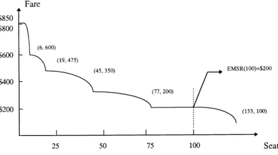
On leg 2, we can get a similar EMSR Curve:

(34)

Fare (6, 600) *\ (19,475) (45, 350) $850 $800 $600 $400 $200 25 50 75 100

Figure 2.5 EMSR Curve Based on Pseudo Fares on Leg 2

EMSR(100)=$200

From the two figure above we can easily determine that the seat protection for class. They are listed in Table 2.19.

each virtual

Y1 Y2 Y3 Y4 Y5

Seats Protection on Leg 1 7 15 41 69 124

Seats Protection on Leg 2 6 19 45 77 133

Table 2.19 Seats Protection in the Non-greedy Virtual Nesting Method

If we assume that the capacity on both legs is 100 seats we will have the following booking limits.

Y1 Y2 Y3 Y4 Y5 Y6

Booking Limits on Leg 1 100 93 85 59 31 0

Booking Limits on Leg 2 100 94 71 55 23 0

Table 2.20 Booking Limits in the Non-greedy Virtual Nesting Method

The critical EMSR value on leg 1 and leg 2 are $150 and $200, respectively.

By comparing the results we achieved here with those obtained from greedy virtual nesting, we find that some of the long haul connecting passengers no longer have a higher priority than the local passengers, and the connecting

Q

class is ranked in the lowest

(77, 200)

(133, 100)

(35)

virtual class without seat availability at all. On the other hand, the local

Q

class passengers on both legs have seats available at this time. This observation also differs from the results we obtained from the heuristic bid price.

2.4.2 Summary

The non-greedy virtual nesting method employs simple network LP concepts to calculate the shadow prices, and to measure the displacement impact of the connecting passengers. Such a strategy normally performs well when demand is extremely high. However several issues need to be taken into account when we calculate the shadow prices, and we will discuss them in Chapter 3.

2.5 Network Deterministic Bid Price

The four methods introduced above used the concept of heuristic nesting. The method we will address in this section is a pure network optimization process. Its concept is similar to that of the heuristic bid price. The difference is that it uses the shadow prices directly as the bid prices on each leg. We will use the previous example to explain this approach.

2.5.1 Process of the Method

First, solve the LP equation [2.2] as we did in section 2.4.1 and get the shadow prices on each leg. The results are:

Spiegi = $150 [2.10]

SPeg2 = $200

The principles for booking decisions in this method are: for local passengers, if their fare value is higher than the shadow price on the leg they traverse, they are booked; for

(36)

connecting passengers, they can be booked if and only if their fare values are greater than the sum of the shadow prices on all legs they traverse. So, we have the following three booking decision tables.

Local passengers on leg 1

Y 500 200 Book

B 300 200 Book

Q 150 200 Spill

Table 2.21 Booking Decisions for Local Passengers on Leg 1 Local passengers on leg 2

Y 600 150 Book

B 350 150

Book-Q 200 150 Book

Table 2.22 Booking Decisions for Local Passengers on Leg 2

Connecting passengers

Y 800 200+150 Book

B 500 200+150 Book

Q 250 200+150 Spill

Table 2.23 Booking Decisions for Connecting Passengers

2.5.2 Summary

The network bid price method uses the LP network optimization concepts to establish the bid prices. One problem of utilizing this model is that, in the formulation of the

optimization model, the right-hand sides of the constraints require the remaining capacity on each leg and forecast future demands of each OD fare class. This information changes during the booking process for a departure date. Therefore, to use this method requires the airline to run the LP frequently. This is impractical because most airlines do not have the data to support such a dynamic optimization process. Plus, running an LP is very time consuming as the network grows larger and larger.

(37)

2.6 Chapter Summary

In this chapter, we introduced five different revenue management methods:

The Leg Based Fare Class Yield Management Method directly utilizes the existing fare classes to calculate the EMSR booking limits. It is simple to employ and therefore is practiced by many airlines. However, this method ignores the fact that the long haul connecting passengers normally provide more revenue than the short haul local passengers.

The Greedy Virtual Nesting Method treats the fares based on their absolute values and re-arranges the fares to the so-called virtual buckets. In such a way, the long haul connecting passengers obtain the highest priority to access the seats. The greedy method performs well when the demand is low, however when demand is high, booking one connecting passenger may cause two or more local passengers to be spilled, that is, the connecting fares have displacement impacts.

The Greedy Heuristic Bid Price Method takes approximates the displacement impacts of the connecting fares by applying higher bid prices for the connecting passengers than the local passengers. However this method is still a greedy method because the critical EMSR values are calculated based on the total fares.

The Non-greedy Virtual Nesting Method uses the shadow prices from the linear

programming models as the displacement impacts. The advantage of this method is that it gives high revenue contributions (from the simulation results in Chapter 4), but the

disadvantage of this method is that it requires more information in terms of more detailed ODF demand forecasts, at least for the total demand on a network.

The Deterministic Bid Price method is a pure network optimization method, which simply uses the shadow prices from the LP model, therefore it requires more detailed incremental ODF forecasts by booking period.

These five methods, each with its own advantages and disadvantages, suggests a clear research direction: How the connecting fares should be treated under different demand circumstances. Ideally, when the demand is low, the connecting passengers should have

(38)

higher priority to access the seats than the local passengers, while when the demand is high, enough seats should be reserved for the high yield local passengers. In next chapter, we will follow these ideas and propose three new models. We will also discuss how to avoid over-emphasizing the displacement impacts of the connecting passengers in practice.

(39)

Chapter 3 Approaches to Network O-D Control

Considering Displacement Impacts

The mathematical approaches reviewed in the previous chapters suggest directions for developing new seat inventory control methods. For example, in the non-greedy virtual nesting method, the displacement impact of the connecting passengers is taken into account by employing an LP model. Are there any better ways to evaluate such effects? Can we take advantages of several good methods to achieve the best revenue performance? In this chapter, the methodologies of several new models are presented. A simple network (Figure 2.1) will be employed to explain how to apply these methods in practice, and several related subjects will be explored.

3.1 Non-greedy Heuristic Bid Price Control

Model

3.1.1 Introduction

We propose this new model based on two observations about the previously reviewed airline seat inventory control methods:

1. The greedy virtual nesting method does not perform very well when the demand is extremely high, because under such conditions, booking one connecting passenger may

(40)

cause two local passengers to be spilled. We know that, normally, two local passengers have a higher total revenue contribution than one connecting passenger. This

observation tells us that the total itinerary network revenue contribution of the

connecting passengers should not be their total itinerary fares, if they make any negative revenue impact on the network. In order to evaluate such negative impacts, we have to solve the LP to calculate the shadow prices associated with the capacity constraints.

2. The heuristic bid price method has shown positive revenue performance in practice', which we ascribe to the consideration of the displacement impacts of the connecting passengers through setting a higher bid price for them than for local passengers.

However, it is still based on a greedy virtual nesting method, and the total itinerary fares are utilized to calculate the critical EMSR values.

The new model, which we name Non-Greedy Heuristic Bid Price method, inherits the merits of both non-greedy virtual nesting and the greedy heuristic bid price methods. In this

approach, we calculate the pseudo fares first, then obtain the critical EMSR values and the bid prices.

3.1.2 The Model

The main idea of this new model is that we will incorporate the displacement impacts of the connecting passenger by using the pseudo fares to calculate the critical EMSR values. This is the same as the non-greedy virtual nesting method. Then, in the next step, the heuristic bid prices are utilized to decide the booking limits.

A broad definition of the shadow price is "the maximum amount that a manager should be willing to pay for an additional unit of resource."2 In our deterministic LP optimization model, the shadow price is the value of the last seat on each leg, and it is positive only when spill is expected to occur.

In the non-greedy virtual nesting method (reviewed in Chapter 2), the pseudo fares, which are defined as fares minus shadow prices, are introduced to reflect the total itinerary revenue contribution of the passengers. For local passengers, their pseudo fares are identical to their

' P.P. Belobaba, Airline O-D Seat Inventory Control Without Network Optimization, Flight Transportation Laboratory, MIT, Cambridge, MA, June 1995.

2 W.L. Winston, Operations Research, Application and Algorithms, Third Edition, Duxbury Press, Belmont,

(41)

total fares since they do not make any displacement impacts, while for the connecting passengers, their pseudo fares will be less than their total fares if the shadow prices are positive (or spills are expected).

An alternative way to evaluate this displacement impact of the connecting passengers is to utilize the critical EMSR value on each leg. The critical EMSR value is a marginal value of the last seat on a leg.

EMSR(S)= f -P(S) [3.1]

where the EMSR(S) is the expected marginal seat revenue of the Sth seat,

f

is the fare value, and P(S) is the probability that the Sth seat can be occupied by the passengers paying faref The EMSR is a measurement of the value of the last seat on a leg, and we can employ it to gauge the displacement impact of a connecting passenger. Therefore we will be able to define the pseudo fares in another form, that is, fares minus the critical EMSR values.

Since there are two alternatives to evaluate the displacement impacts of the connecting passengers--the shadow prices from network optimization and the critical EMSR values from leg based probability optimization--we can divide our model into two sub-methods: the Network greedy Heuristic Bid Price Method and the Leg-based Probability Non-greedy Heuristic Bid Price Method.

1. Network Non-greedy Bid Price Method

In this method, the shadow prices are calculated from solving a deterministic linear program, then the pseudo fares are employed to evaluate the revenue contribution of the passengers to obtain the critical EMSR value on each leg, and consequently, the bid prices are decided.

For the local fares, the bid prices are simply the EMSR values on the corresponding legs, while for the connecting fares, the bid prices on Leg 1 are:

BP = EMSR,+d x EMSR2, [3.2]

while the bid prices on Leg 2 are: