HAL Id: hal-01585974
https://hal.archives-ouvertes.fr/hal-01585974
Submitted on 12 Sep 2017
HAL is a multi-disciplinary open access archive for the deposit and dissemination of sci-entific research documents, whether they are pub-lished or not. The documents may come from teaching and research institutions in France or
L’archive ouverte pluridisciplinaire HAL, est destinée au dépôt et à la diffusion de documents scientifiques de niveau recherche, publiés ou non, émanant des établissements d’enseignement et de recherche français ou étrangers, des laboratoires
Cross-commuting and housing prices in a polycentric
modeling of cities
Vincent Viguie
To cite this version:
Vincent Viguie. Cross-commuting and housing prices in a polycentric modeling of cities. 2015. �hal-01585974�
Cross-commuting and housing prices in a
polycentric modeling of cities
Viguié Vincent
WP 2015.09
Suggested citation:
Viguié Vincent (2015). Cross-commuting and housing prices in a polycentric modeling of cities?
FAERE Working Paper, 2015.09.
ISSN number:
Cross-commuting and housing prices in a polycentric
modeling of cities
Vincent Viguié
a,1,⇤aCIRED (Centre International de Recherche sur l’Environnment et le Développement), Ecole des Ponts ParisTech, Paris, France
May 26, 2015 Abstract
Long term strategies, relying on city planning and travel demand management, are essential if deep GHG reduction ambitions are to be achieved in urban transport sector. However, how to precisely design such strategies remains unclear. Indeed, whereas there is a broad consensus that urban spatial structure is a key determinant in explaining travel pattern generation, the mechanisms are not yet fully understood. Especially, the interplay between commuting and localization choices leading to cross commuting in a polycentric city remains an open question, and cannot be easily explained using existing urban economics frameworks. In this study, we introduce a novel urban economic framework, fully micro-economic based, which describes land prices, population distribution and commuting travel choices in a polycentric city, with jobs locations exogenously given. It relies on the modeling of moving costs and market imperfections, especially housing-search imperfections. Using Paris as a case study, we show how this model, when adequately calibrated, reproduces available data on the internal structure of the city (rents, population densities, travel choices). A validation over the 1900-2010 period also shows that the model captures the main determinants of city shape evolution over this time. This suggests that this tool can be used to inform policy decisions.
Keywords: urban economics, cross-commuting, urban planning, climate change mitigation JEL: Q5, R14, R4
1. Introduction
Transport is one of climate change key issues. It is indeed responsible for a large fraction (23%) of total energy related CO2 emissions in the world, and this share is increasing (energy use for transport has increased at a faster rate than any other energy end use sector since 1970) (IPCC, 2014b). Urban transport alone is responsible for about 40% of global transport-related energy use, and urgent and sustained mitigation policies are required in this sector (IEA, 2013). Together with short term mitigation actions, on modal choice or vehicle efficiency for instance, long term strategies, relying on city planning and travel demand management, are essential if deep
⇤Corresponding author
Email address: viguie@centre-cired.fr (Vincent Viguié)
1Tel: (33) 1 43 94 73 79 Fax: (33) 1 43 94 73 70, CIRED, Site du Jardin Tropical, 45bis, Av de la Belle Gabrielle
GHG reduction ambitions are to be achieved (Schafer,2012). Several studies illustrate how urban shape (i.e. the way a city is spatially organized, its density for instance) impacts urban transports emissions through an action on modal choice and on transport demand (Cao et al., 2009;Ewing and Cervero, 2010;Echenique et al., 2012). This is particularly visible at the aggregate level, as GHG emissions from land transport in cities inversely correlate with urban population densities (Newman and Kenworthy,1999;Rickwood et al.,2008;Kennedy et al.,2009).
However, whereas there is a broad consensus that urban spatial structure is a key determi-nant in explaining travel pattern generation, the mechanisms are not precisely known. Most metropolitan areas across the world are experiencing continuous increase in annual average pas-senger km per capita, and commuting journeys, which constitute an important part of these travels, have largely followed these general trends (Aguiléra et al.,2009;IPCC,2014a). A better under-standing of the mechanisms at stake and the determinants of travel demand is necessary if one wants to contain this growth.
"Excess commuting" (or "wasteful commuting") epitomizes this lack of understanding. This concept was initially introduced byHamilton(1982),2and has become a well-established research
field in the subsequent decades (Ma and Banister,2006). It represents home to work travels "in ex-cess" of what should be the case according to urban economic models and housing expenses/travel generalized price joined minimization which is at their core: this minimization indeed excludes the existence of cross-commuting between job centers, whereas in practice it is widely observed. Numerous studies have empirically examined this phenomenon, developing methods to measure it (see for instanceMcMillen, 2001;O Kelly and Lee,2005;Van Ommeren and Van der Straaten, 2005;Horner,2008), and studying its main characteristics, such as its magnitude in different cities around the world, or its evolution over time (Ma and Banister, 2007). Depending on how it is measured, this excess commuting can be far from negligible, and represent more than half of the total commuting travel distance in the city (Ma and Banister,2006;Boussauw et al.,2011).
A number of potential explanations have been proposed in the literature to explain the dis-crepancy between urban economics models conclusions and actual travel patterns. However, the respective influence of these factors, as their precise consequences, is not yet fully understood (Ma and Banister, 2006). One reason lies in the fact that only a few of these mechanisms have been successfully included into urban economics framework. One of the main fruitful direction was given byAnas (1990) and Martinez(1992), and proposes to introduce idiosyncratic preferences for the different locations inside the city. This leads to cross-commuting and population mixing, i.e. everywhere in the city can coexist different households working at different locations.
In this paper, we introduce a novel approach, and show how it is possible to include a new mechanism causing excess-commuting into urban economics framework. This approach proposes to explicitly model moving costs and market imperfections, especially housing-search imperfec-tions, to account for cross-commuting. It leads to a modeled city which is broadly comparable to what is obtained through the use of idiosyncratic preferences. However, both frameworks lead to differing conclusions for a few key points.
Using Paris urban area as a case study, we show how the model that we propose can reproduce available data about rents, population densities, and travel choices. It can also capture some of the
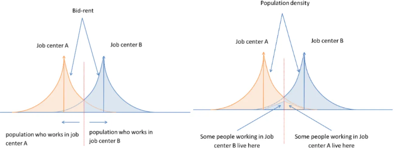
(a) Bid-rents and population-job match in a classical
urban economic model with several job centers. (b) Illustration of possible excess commuting.
Figure 1: Classical urban economics model and excess commuting.
characteristics of the evolution of the city since the beginning of the XXth century. This suggests that this tool can be used to inform policy decisions.
Section2presents the context of our work, and sums up how existing polycentric urban eco-nomics models describe travel choices. Section3presents our model, and section4its calibration over Paris urban area, and especially how this model simulates cross-commuting. Section5 con-cludes.
2. Polycentric modeling of cities
2.1. Urban economic framework and polycentric modeling
Classical urban economics framework is an economic modeling approach developed initially at the end of the 1960s (Alonso,1964;Mills,1967;Muth,1969; a pedagogic introduction can be found inFujita,1989orBrueckner,2012) which aims at explaining the spatial distribution - across the city - of the costs of land and of real estate, housing surface, population density and buildings heights and density. It considers monocentric cities, i.e. cities where everybody is working at the same place. In this framework, people working in a certain location are willing to pay less for accommodation when they live far from their job: the further they live, the less they are willing to pay. The amount they are willing to pay is called the bid-rent. If landowners choose rents in each point to maximize their profit, rents are equal to this bid-rent.
There are several ways to extend this framework to a polycentric case, i.e. when there are several job centers in the city. First, it is possible to associate a bid-rent curve to each job center. Landowners then determine rent level using the maximum bid-rent at every place. In such a case, people only inhabit in places where rent is equal to their bid-rent, and this leads to a perfect segregation of people in the city, based on their place of work (figure1a).
In practice, however, such a configuration is not realistic, and two main discrepancies have to be noted. This is the basis of the debate about “excess commuting” we mentioned in Introduction.
First, in such a model, households live immediately around their place of work, whereas in practice many households live far from their place of work, but close to the place of work of other people (see sec. 2.2). Second, in the model, the city is divided in zones where households have the exact same work location, whereas in practice they are mixed: it is the “population mixing” issue (see sec. 2.3).
2.2. Commuting in excess
In a literature review, Ma and Banister(2006) list main factors which could explain the first discrepancy, and prevent urban workers from finding nearby jobs or residential locations, thus causing excess commuting:
(i) Multi-worker households : The increasing prevalence of two-worker households imposes trade-offs between commuting distances of each worker, as optimizing one worker’s com-mute may increase that of the other.
(ii) Rapid job turnover versus high transaction costs of house relocation : This can lead house-holds not to be able to fully optimize their home location with respect to their present work location.
(iii) Heterogeneity: Heterogeneity in population behavior, preferences, choices or possibilities can also generate travel patterns different from what would result from a simple optimization supposing that all households are identical. Examples include heterogeneous housing and job markets, different tax subsidy systems, minority groups...
(iv) Neighborhood amenity and decreasing importance of commuting: Households do not only choose their residence location based on commuting trips: the rise of telecommuting, the increasing importance of non-work trips, and the influence of neighborhood amenity also contribute to the existence of this excess commuting.
(v) Psychological dimension: People may want to separate homes from workplaces, and may value the time taken to commute. This idea is supported by the invariability of average travel times that is found in many cities, regardless of the widely differing income levels, geog-raphy and transportation infrastructures (Zahavi and Talvitie, 1980; Levinson and Kumar, 1994;Schafer,1998;Schafer and Victor,2000;Mokhtarian and Chen,2004;Metz,2008). The respective influence of these factors, however, is not yet fully understood, and as Ma and Banister (2006) note, it is generally assumed that “the inflexibility of the labour market, more black and minority workers in the urban labour force, a decrease in the mobility of workers, and the growing non-work trips are all likely to increase the amount of excess commute”.
Several models have illustrated how such mechanisms could be included into urban economics framework. Multi-worker household is a relatively simple extension to the monocentric model (see for instanceKim, 1995), as is heterogeneity in households characteristics (see for instanceFujita (1989) or all the literature about spatial mismatch, such asGobillon et al.,2007). Local amenities role is illustrated byNg (2008), telecommuting by Rhee(2008) and anticipation of potential job change byCrane(1996).3
3About anticipation of potential job change, see alsoSong(1995);Anas et al.(1998). These articles deal with urban
All these mechanisms can lead to excess commuting, but do not explain population mixing, however. They lead to the description of cities as spaces fully segregated in zones populated exclusively by households with the same exact characteristics (Wheaton,2004). Indeed, in urban economic framework, the choice of who inhabits the land at each location is deterministically determined based on who offers the highest rent : the inhabitants are therefore exclusively of one type except in the case where the rent from two household groups is strictly identical. This creates land use patterns in which there are exclusive zones or rings for each household group.
2.3. Population mixing
This population mixing issue has been somehow less studied in the literature. Different models have been developed to account for it. They generally assume that it results from the existence of a very large number of households characteristics, instead of a small number of possibilities. Conceptually, the city is still divided into multiple zones of homogeneous pattern, but each zone is in practice reduced to one, or a few, households. Taking into account explicitly a great number of characteristics, however, generally leads to computations which are intractable analytically.
One method to bring back analytical tractability is the supposition of the existence of a con-tinuum of households characteristics, instead of a finite number of possibilities. Including such a continuum could be done for all the mechanisms we have listed in previous section. However, the mathematical (and conceptual) derivations are not straightforward, and as a result it has only been achieved for some of these mechanisms.4
In such frameworks, the distribution of the characteristics over the population is treated prob-abilistically, and the choices of any one household can be determined only probabilistically. As stated byAnas (1990), "equilibrium is not characterized by a statement of exactly where a par-ticular household locates but rather by a probability distribution which gives the odds that the representative (randomly selected) household chooses a particular location. Such a stochastic de-scription of equilibrium does not imply that behavior is not deterministic, but only that the essential aspects of such an equilibrium are revealed and analyzed in stochastic terms."
Let us briefly describe now how population mixing has been modelled in the literature: Job change. A first idea is to model job changes anticipations. This can be done with a straight-forward extension of the standard urban economic model. The idea is to suppose that households first choose their place of residence before choosing their place of work, and that, because of some transaction costs or unobserved idiosyncratic characteristics, they cannot fully optimize their job location.
4In regard to the mathematical difficulties it raises, one could wonder if it is actually useful to look for analytically
tractable models here. Numerical simulations are indeed an adequate tool to analyze the consequences of the existence of different households characteristics (see for instanceLemoy et al.,2010,2013). Through such simulations it is in theory possible to include as many households characteristics as one wants, and to observe how this influences the city. However, such simulations can only enable to study a finite number of cases, and not to rigorously infer the consequences of generic assumptions. Also, from a practical point of view, such simulations quickly become extremely computationally intensive if many households characteristics have to be taken into account. This limits in practice the number of these characteristics, and the possibility to efficiently represent population mixing.
This is modeled by supposing that there is an accessibility to jobs associated with each loca-tion in the city, and that households willingness to pay is determined by this accessibility. Once someone locates somewhere, the actual job to which he is commuting to is selected, through some given rule, among all jobs accessible from this location.
Let us take an example: job distribution being given in a city, it is possible to suppose that once someone locates in location x, the probability that he will have a job located at a distance d decreases with d. Let us call P(d) the probability to accept a given job at a distance d. Knowing this rule, the inhabitant will anticipate that, if he locates in x, his expected future commuting distance will be
E(d) = Âjd.P(d) ÂjP(d)
where Âj is the sum over all jobs. It is therefore possible to use classical urban economic framework, replacing travel costs to go to work with expected travel costs to go to potential future job. Once people are located in the city, actual job choice is given by probabilities P(d), which means that at any given location there will be people working in different places, i.e. there will be population mixing. However, the main drawback of this type of model is the fact that it is not possible to control that the number of households selected to work at a given place actually corresponds to the number of jobs in this location.
Idiosyncratic taste constant (random utility models): discrete choice approach. One of the most fruitful derivation, by Anas (1990)5, considers a continuum in households preferences for local amenities. This model has been used to analyze conceptual issues (Anas and Rhee,2006, 2007), and has led to applications in operational, calibrated models (Anas, 2013). It proposes to add to classic urban economics utility U a stochastic idiosyncratic taste constante which differs among locations for each household and differ among households for each location:
˜
U(x) = U(Z(x),q(x)) +e(x)
where the deterministic part U(Z(x),q(x)) is a classical utility function on demand of the composite commodity Z and lot size q. As proven byAnas(1983), ife(x) follows a type 2 Gumbel distribution, this formulation leads to the same home-job pairing as gravity models, which describe relatively well commuting trips observed in practice.
Such an approach results in rent and density profiles which differ from the profiles induced by plain urban economic theory: the heterogeneity of tastes flattens the rent and residential density gradients, and decentralizes the city. A higher degree of heterogeneity in tastes also results in a higher level of welfare for the representative consumer. (Anas,1990)
However, this approach has a few drawbacks. First, rents are computed at each location as the prices which equalize expected demand and supply of housing surface. They are therefore not determined as the result of landlords profit-maximization, and no mechanism explains why higher rents could not be preferred.
5See also extensions inAnas and Kim(1996) to include congestion and job agglomeration, and inTscharaktschiew and Hirte(2010) to include different households classes
The second drawback is deeply related to the first. It comes from the fact that, to apply this model, it is necessary to aggregate together different locations across a city (all the locations of a neighborhood, say). However, the number of zones, i.e. the choice in the aggregation level, has a deep influence on the outcome of the model. A solution, introduced by Wrede (2014), is to consider the limit in which each zone is infinitely small, i.e. to consider a continuity of taste constant with respect to space. This approach seems promising, however the model then becomes extremely complex from a mathematical point of view, and has only been applied so far to a schematic city with a particular geometry (a star-shaped city).
This has another, more practical, consequence. The link between transport and rents is im-plicitly stated in this framework, and is far from being as direct as in standard urban economics models. To solve this model (either analytically or numerically), for each household class type, as many equations have to be solved as there are locations in the city, because each rent level is the solution of an equation. This makes this model rapidly analytically intractable and extensive simulations are required as soon as the number of zones becomes big.
When such a model is calibrated on an actual city, this therefore limits in practice the number of zones among which the city has to be divided, i.e. the spatial resolution of the model cannot be too fine. For instance, Anas (2013) explains that when RELU-TRAN, a land-use transport interaction model based on this framework, was calibrated on Paris urban area, it divided the city into about 50 zones. This may be a problem when city description at a smaller scale is needed (as a comparison, the model that we describe in Section4divides Paris urban area into 10000 zones). Idiosyncratic taste constant (random utility models): Stochastic bid-rent model. Another formu-lation, the stochastic bid-rent model, relies on a similar idea. It was first proposed byEllickson (1981), studied in-depth by Martinez (1992), and has been included into calibrated operational models, especially MUSSA (Martinez et al.,2007).
It partly addresses one of the issues of the last approach: the lack of profit-maximizing mecha-nism explaining rents formation. Actually, this formulation gives exactly identical results, in terms of rent level and population density, as the discrete choice approach, a result proven byMartinez (1992). It can therefore be considered more as another way to interpret a common mathematical framework than as another framework.
As in previous case, the idea is to consider a stochastic idiosyncratic utility which differs among locations for each household and differs among households for each location. However, it is written in a different form. When utility U(Z,q) is deterministic, if we introduce a budget constraint Y = Z + q.R, it is possible to write the indirect utility function, which includes this budget constraint by expressing composite good Z as a function of income Y , rent R and housing size q. It is then possible to build a willingness to pay functionQ(u,Y,q) which is equal to the rent R that a household would accept to pay to reach utility level u, given income Y and house size q. In other terms,Q is the function which solves the equation U(Y q.Q,q) = u.
In the standard urban economics model, Q is households bid-rent. In stochastic bid-choice model, we suppose that households bid with function
˜Q = Q+e(x)
choose rent level as the maximum of these willingness to pay functions, i.e. maximize their in-come. Ife(x) follows here again a type 2 Gumbel distribution, then rents and population location choices become equal to what they were is the last framework.
This approach provides an explanation of the mechanism through which rents are determined. However, it suffers from the same drawbacks as the previous approach: it is not easy to establish the explicit interaction between land-use and transport, the choice of the aggregation level has a deep influence on the outcome of the model, and when calibrated on an actual city, the city has to be divided into a relatively small number of zones.
Another drawback exists, also, because this framework only explains the relative variation of rents across a city, but cannot determine the absolute level of rents. The mechanism considered here to explain the determination of rents explains why rents are higher in some places than in another, and what is the difference. However, rigorously speaking, this mechanism leads to rents being uniformly much higher than they are in reality.
The intuitive reason is as follows. Let us suppose, as a simple case, that the city is populated by people with the same utility function (i.e. there is only one type of household). Let us consider a given location in the city. At this location, each household will bid for housing, and the bid will be given by the function ˜Q. Since all households have the same utility function, the deterministic part, Q, will be the same for each of them. However, the stochastic term, e, will be different, and follows a probability distribution. If this value follows a type 2 Gumbel distribution (or any non-bounded distribution), there is a non-zero probability that at least the terme of one of the household is very big. To say things differently, if the population is sufficiently large, the probability that, in any given location, at least one person can agree to pay an absurdly large rent, i.e. has a large e(x), may not be small. Since rents are given by the maximum of the bid-rents, i.e. by the maximum of thee(x), nothing prevents rents from being extremely high everywhere.6
The only way to prevent this is to suppose that the stochastic terme(x) is not centered on 0, but centered on a large negative value, which depends on the total number of households in the city (Martínez and Henríquez,2007). This approach is not fully satisfying as it imposes to relate utility function of each household to the number of other households in the city.
As with the discrete choice approach, developments have taken place to improve this model, especially through the use of game theory to add more realism to the bidding process and competi-tion between households for the maximum bid (see for instanceChang,2006;Chang and Mackett, 2006).
6Here is the rigorous mathematical explanation. Ife(x) follows a Gumbel distribution with location parameter µ
and scale parameterl (i.e. probability distribution function f (x) = l.e l(x µ).e e l(x µ)), then the expected value of
e(x) is E[e(x)] = µ + 0.5572...l (where 0.5572... is Euler constant). If there are N households, and if, for all of them, e(x) follows the same distribution, the expected value of the maximum of the e(x) is E[maxNe(x)] = 1llog(N) + µ +
3. A polycentric framework based on moving costs and housing-search imperfections mod-eling
3.1. Our approach
We propose here a new approach not relying on idiosyncratic local amenities, but based on the modeling of moving costs and market imperfections, especially housing-search imperfections. As noted in section2.2, this is one of the explanations proposed in the literature to explain excess-commuting (Van Ommeren and Van der Straaten,2005).7
The approach presented here is not meant to supplement previous approaches, but rather to complement them. Idiosyncratic taste constant approaches model the point 4 "Neighborhood amenity" of section2.2. We propose here to model the point 2 "Rapid job turnover versus high transaction costs of house relocation". Ideally, this framework should be included in a wider framework, taking into account all five points. This would enable to analyze more finely how the mechanisms interact, and their respective amplitude in different cities and over time.
This model is not an equilibrium model : we consider that the city never fully reaches equi-librium, and that what is observed over the long term is steady state.8 To analyze the effects of
transaction costs, we suppose that households who want to relocate compare their present utility with the utility they could get if they relocate. Such an approach, based on household residential search modelling, enables to take transaction costs explicitly into account (cf. Weinberg et al., 1981;van Ommeren et al.,1997).
Finally, similarly to the approaches listed in Sec. 2.3, the model gives probabilistic results: it does not determine the choices of each individual household, but enables to compute averages at each location.
3.2. Principle
Let us describe briefly the intuition behind the model. We first suppose that households regu-larly want to relocate in the city, for instance because they change job. When households relocate, however, they can only choose among a limited number of available dwellings.
More precisely, we suppose that, from time to time, a new dwelling is proposed on the market with a given rent. At this time, several households want to relocate : some of them might find this dwelling acceptable, and some other will prefer to wait more time to find a better dwelling.9
7It is interesting to note that two main empirical findings support this hypothesis: first, there is a link between job
turnover and commuting distance (those who have relatively unstable jobs are likely to have longer commutes:Crane,
1996;Van Ommeren and Van der Straaten,2005,2008), and, second, home-owners have higher excess commuting levels than renters (Kim,1995).
8Looking at steady state and not equilibrium is a convenient approach used for instance inWheaton(1990), in a
study of the link between housing vacancy rate and housing prices.
9There is another another way to consider the difference between the approach that we propose here and the
id-iosyncratic taste constant approach. The latter corresponds to horizontal sorting between neighborhoods (heterogene-ity across individuals in preferences for specific neighborhood attributes). On the contrary, our approach corresponds to vertical sorting (everyone agrees on differences in choices, but there is an heterogeneous willingness to pay for the process of location optimization, i.e. for neighborhood quality versus other types of consumption).
Households behavior. Here is how this can be more rigorously expressed: when relocating in the city, we suppose that households try to maximize their utility. Let us call U⇤the maximum utility they could get in the city. Because there is a cost for households to wait for an optimal dwelling to be available, however, we suppose that households do not automatically choose a dwelling which gives them their maximum utility U⇤: we suppose that households accept to settle in a place where they can get a utility U U⇤with a probability P(U,U⇤), where P(U⇤,U⇤) =1.10
Let us also suppose that, at each time step, the number of households who want to relocate is equal to a given fraction f of households working in each job location. In this case, the number of households working in job center i who will find acceptable a given dwelling at a location x with a size q and a rent R is
f .Ni.P(Ui(x,q,R),Ui⇤)
where Niis the number of households working in job center i, Ui(x,q,R) the utility that they could get in x with housing size q and rent R, and U⇤
i the maximum utility they could get in the city. Finally, let us suppose that when a dwelling is available, if several households who want to relocate find this dwelling acceptable and therefore compete for it, then this dwelling is randomly given to one of the competing households. In this case, when a dwelling in a location x with a rent R is available, the probability that a household working in i moves in it is :
Pi(x,q,R) = f .Ni.P(Ui(x,q,R),U ⇤ i ) f . kNk.P(Uk(x,q,R),U ⇤ k) = Ni.P(Ui(x,q,R),Ui⇤)  kNk.P(Uk(x,q,R),U ⇤ k) (1)
If rent R is the same for all dwellings at the same location (i.e. for a given x, R is given), then after some time steps the city will converge towards a stationary state, in which Eq. 1 gives the distribution of households at each location.
Land market clearing. Let us describe in more details landlords behavior. We suppose that each landlord owns one dwelling. It takes housing quantity H(x), household income Y and transport costs as given, and chooses rent R to maximize its income. More precisely, landlords maximize their income under the constraint that their dwelling must be occupied, i.e. when the dwelling becomes available, there has to be at least one household who wants to relocate and finds this dwelling acceptable.
We suppose that landlords, unfortunately, have to choose rent level R before knowing which utility levels U will be acceptable for households. These utility levels are randomly distributed, and landlords only know their probability distribution P(U,U⇤): landlords have to decide the rent R before these levels are revealed. To be sure that at least one household will find the dwelling acceptable, landlords therefore have to propose a rent R such that, for at least one job center i, Ui(x,q,R) = Ui⇤.
As in section2.2, people working in a given job center j are willing to pay less if they locate further from their job center, and there is a bid-rent Yj(x,U⇤j) associated with each job center, which gives rent level corresponding to a constant utility. This means that there needs to be at
10For consistency, the probability function P should also be equal to zero in places where households cannot relocate
least one job center i for which R =Yi(x,Ui⇤), and rents will therefore be simply given by the maximum of all bid-rent:
R(x) = max
i2JobcentersYi(x,U ⇤
i ) (2)
Similarly, we assume that when landlords choose the rent, they simultaneously choose the size of the flats they propose on the market. They choose this size so that it corresponds to the size q which maximizes the utility of the households working in job center i (where job center i is the job center whose households have the highest bid-rentYi(x,U⇤
i)).
3.3. Comparison with classical urban economics and idiosyncratic taste constant approaches To sum things up, in a "classical" urban economics framework with several job centers, the city is divided in homogenous zones, centered around each job center, in which inhabitants all work in the same center. There is a bid-rent curve associated to each job center, and rents are given by the maximum of these bid-rent curves (i.e. rents are maximum close to each job center, and decrease when moving away from them, cf. Fig.1a).
In our framework, rents are given by the exact same principle. They are in fact strictly equal to what they would be in the "classical" urban economics framework. It is the same for dwelling size per household, and, therefore, for population densities across the city. However, the city is no longer divided in homogenous zones, as everywhere in the city coexist people working in different job centers (it is actually well represented by Fig.1b). At a given location x in the city, the fraction of people working in job center j is given by Eq. 1.
These two facts (housing prices similar to "classical" urban economics framework, but land usage impacted by the proximity to all job centers) are consistent with empirical findings (see Muto,2006, about Tokyo), but, to the author’s knowledge, only one study empirically addresses this issue. These results differ from what is obtained in idiosyncratic taste constant approaches. In these approaches housing prices are not similar to housing prices obtained in "classical" urban economics framework, as they are for instance asymmetric around secondary business centers (Wrede,2014).11
More importantly, in our approach, utility of households working in the same job center is not uniform across the city, whereas this is by hypothesis the case in idiosyncratic taste constant approaches, and in "classical" urban economics framework. Specifically, in our approach, utility tends to decrease whith the distance between housing and job location. Indeed, the further from a job center, the higher the probability the highest bid-rent is not the bid-rent associated to this job center.
In recent years, a few empirical studies have tried to measure the relationship between com-muting and well-being, using declared subjective well being as a proxy for individual welfare. Commuting in itself is detrimental to well-being, but these studies examined something differ-ent. They examined whether individuals with longer commutes tend to report lower levels of life
11Two empirical articles (Osland and Thorsen,2008;Ahlfeldt,2011) show that gravity employment accessibility
measures provide a good explanation for land and housing prices in Berlin and Rogaland County in the southwest of Norway. This is coherent with idiosyncratic taste constant models results. It is therefore difficult to say that empirical findings of land and housing prices favor one approach or the other (or a combination of both).
satisfaction, i.e. if longer commutes are compensated in some way, in the form of improved job characteristics (including pay) or better housing prospects, for instance. Stutzer and Frey(2008) were the first to look at this question, and found a decreasing well being with the distance between housing and job location. They called it “The Commuting Paradox” as it it not coherent with classical urban economics theory (and neither with idiosyncratic taste constant approaches). It is interesting to note that such a result is conversely coherent with our approach.
It should be noted, however, that subsequent works have shown that he relationship between commuting and subjective well-being is complex (Roberts et al.,2011) and may be affected by the measurement method (Dickerson et al.,2014).
The best validation of the model utlimately relies in its capacity to capture commuting trips and rent patterns in an actual city. This is what we do in the next section.
4. Calibration over Paris urban area. 4.1. NEDUM-2D model
Viguié (2012), Viguié and Hallegatte (2012), Viguié et al. (2014) and Viguié and Hallegatte (2014) show how it is possible to capture main characteristics of a mainly monocentric city (Paris) using a simple monocentric urban economic model with endogenous building construc-tion (NEDUM-2D model).
To do this, several constraints have to be taken into account.
• First, the model has to accounts for land-use constraints on the Paris agglomeration (such as, for instance, places where it is forbidden or impossible to build).
• Second, transportation costs have to include monetary costs such as the cost of gasoline and the cost of time, and to be assessed using the spatial structure of the Paris transportation networks (roads and public transport). Households can choose between different transport modes (a discrete choice model is used to compute modal shares).
We use the same approach here, and show how a model based on the polycentric framework we have presented here (and taking into account the constraints we have mentioned) can adequately reproduce main characteristics of an actual urban area.
Model parameters (utility function coefficients etc., see Appendix A) are calibrated over the year 2008. The model, using these calibrated coefficients, is then compared with reality for other years, namely 1990, 1960 and 1900. This aims at partially validating that the model captures important mechanisms driving city shape and organization.
However, this is not an actual rigorous validation, because the data used for calibration and validation are not completely independent : we do not aim here at proving that the model is a valid explanation of reality (we do not prove any causality), but simply that it is coherent with reality, i.e. that it is possible to find parameters such that model simulations fit several city characteristics and their evolution over time.
Data and coefficients. All data and coefficients used in the simulations are summed up in Ap-pendix A. Total population of the city, average household size and average income are given by French statistical institute (INSEE). To compute generalized transport prices, we used data about walking times, actual transport times and prices in public transport (underground, regional trains and suburban trains) and private transport (during rush hours, for an average car). At each location, the generalized transport cost is computed for each transport mode, and a logit weighting is used to compute the modal shares.12 In the simulations, changes in public and private transport prices
lead therefore to modal shifts.
We consider 513 job centers in the simulation. Each of them corresponds to one or several “communes” and “arrondissements” (local administrative districts) of Île de France region (see Appendix A.1 and especially Fig. A.6 for more details). Île de France region, which roughly corresponds to Paris urban area as defined by INSEE (French national statistical institute) extends far from Paris city itself. In the simulation, 20 of the 513 job centers are actually inside the administrative boundaries of Paris city.
4.2. Detailed equations
Utility function. We model people behavior using the following utility function:
U = Zaqb (3)
wherea and b are coefficients (a+b = 1), q the surface of the dwelling and Z the money remaining after the household has paid its rent and a commuting round-trip per day to its job center.
The cost of transportation includes the monetary cost of transportation and the cost associated with the trip duration, which we consider as an actual loss of income. Such a functional form is consistent with the fact that the share of household income devoted to housing expenditures is relatively constant over time and space (Muth,1969;Thorsnes,1997).
People income constraint reads:
Y = Z + q.R + T (4)
where Y is people income, R is the rent per square meter, and T transportation cost (monetary cost added with time cost).
Rents. From equations3and4, it is easy to compute bid-rentsYj(x,U⇤j)associated with each job center (see for instanceFujita,1989) :
Yj(x,U⇤j) = aabbYj UTj(x)⇤ j
!1 b
(5) where Yj is income of people working in job center j and Tj(x) is transport cost to commute between location x and job center j. As explained in section 3.2, at any location x, there needs
12More rigorously, at each location, the logit weighting is computed on each price divided by the minimum price at
to be at least one job center t where Ut(x,q,R) = U⇤
t. This means that there needs to be at least one job center t where R =Yt(x,Ut⇤), and rents will therefore be simply given by the maximum bid-rent:
R(x) = max
k Yk(x,U ⇤
k) (6)
Excess commuting. Many functions P(Uj(x,q,R),U⇤
j)could be chosen. We suppose here that P is a function of the comparison of the relative difference between U⇤
j and Uj(x,q,R): Pj(x,q,R) = e l ✓ U⇤j Uj(x,q,R) U j(x,q,R) ◆k =e l U⇤j (Yj Tj(x) q.R)aqb (Yj Tj(x) q.R)aqb !k (7) where l and k are scaling factors. When the difference between Uj(x,q,R) and U⇤
j is small compared to Uj(x,q,R), Pjis close to 1. On the contrary, when this difference is large, Pj is close to 0. Similarly, Pj is equal to 0 when Uj(x,q,R) = 0, i.e. when transport plus housing costs are superior to households income (i.e. whenYj Tj(x) + q.R).
Using both equation1and equation7, we get:
Pj(x,q,R) = Nj.exp ✓ l✓U⇤j (Yj Tj(x) q.R)aqb (Yj Tj(x) q.R)aqb ◆k◆ ÂkNk.exp ✓ l⇣Uk⇤ (Yk Tk(x) q.R)aqb (Yk Tk(x) q.R)aqb ⌘k◆ (8)
Buildings construction. We assume that absentee landowners own the land, and that they combine land with capital to produce housing. The housing production function reads, in a classical way:
e
H = ALaKeb
where A, a and b are coefficients (a + b = 1), eH the housing surface built, L the land surface occupied by the buildings and eK the financial capital used for construction. If we call H = HeL and K =KLe housing surface and capital per land unit, the benefit of land owners reads therefore :
P = R.H (d + r)K
P is the profit per land unit, r represents the joined effect of real estate capital depreciation and annual taxes payed by land owners on the real estate capital, andd the interest rate.
The metropolitan area boundary is defined by a rent R0, below which it is not profitable to build housing.13 This value corresponds both to other use of the land like agriculture and to transaction
costs in the building and renting process (such as costs associated to the development of new building sites, for instance water and electricity networks extension). We suppose that developers can build only if R R0.
13It is equivalent to suppose that the metropolitan area boundary is defined by a land rent, i.e. by a conditionP > P0
Developers build to maximize their profit: at each point of the metropolitan area they construct, i.e. choose K, to maximizeP under the constraint that He
L ratio is limited by a land-use constraint (see detail inAppendix A).
4.3. Equilibrium
In a classical monocentric urban economics model, the equilibrium can be obtained through a two-step computation (see Fujita, 1989). First, based on transport costs, people utility function, and housing production function, rents and population density are computed for every location as a function of inhabitants (uniform) utility level. Then, if we consider the closed city case, i.e. if one wants to prescribe what is the population of the city, an equation has to be solved: the right utility level has to be found so that city total population in the model (i.e. the sum of simulated population densities at each location in the city) becomes equal to the exogenous prescribed population of the city.14
In our framework, there is a utility level associated to each job center. We consider here a generalization of the closed city case, i.e. we consider that the number of people working in each job center is exogenously given. Similarly to the classical case, the computation of the equilibrium involves two steps. In the first step, rents, population density, and fraction of inhabitants working in each job center are computed at every location in the city. These values are function of the N utility levels associated to each job centers (seeAppendix B).
This enables to compute the simulated number of people working in each job center as a function of the N utility levels. Then, in a second step, a system of N equations has to be solved, to find the value of the N utility levels, so that the number of people working in each job center is equal to the exogenously prescribed numbers.
4.4. Comparison between simulation and data
Let us compare the simulation of Paris urban area evolution between 1900 and 2014 with available data. SeeAppendix Afor a detailed description of data used and of coefficient values. 4.4.1. Internal city structure: rents and population density
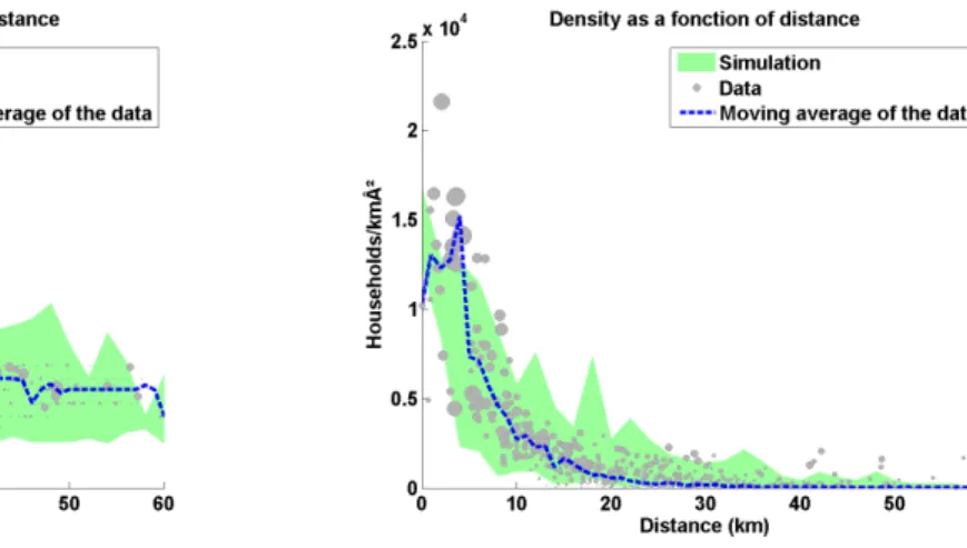
As shown in Fig.2bthe model describes the distribution of population densities across the city in 2008 satisfactorily. Figure2ashows that there is also a good agreement between the model and data in terms of rents. Model and data seem to match well on the urban area scale, even if local differences can be large, due to the lack of several locally-important characteristics (e.g., public services supply and local amenities).
The model appears to underestimate rent levels close to Paris center, and to overestimate rents in the close suburbs (between 5 and 20km). One reason explaining this discrepancy is the fact that the model does not take into account income differences across the city. Indeed, rents are impacted by local households income, and, everything else being equal, tend to be higher in a richer neigh-borhood than in a poorer one. In practice, inhabitants income is in average significantly higher than average close to Paris city center, and lower than average in the close suburbs (Floch,2014):
14The other, symmetric case is the open city case in which the population of the city is not exogenously given, but
(a) Rents in 2008 (Data source: CLAMEUR). (b) Population density in 2006 (Data source: INSEE).
Figure 2: Rents and population density computed by the model (green area) and from data. Dots represent data for individual localities (their size is proportional to the localities populations). The dotted line represents the average value of data at a given distance from Paris center.
the consequences of this income variation cannot be captured by the model. Correspondence be-tween model simulation and reality is greater in Fig. 2bbecause local population density is less impacted than rents by local inhabitants income.
4.4.2. Internal city structure: excess commuting
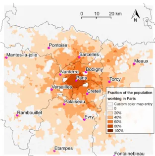
Fig. 3compares home-work distances in the simulation and in data. In each place, there is a mix of people working in different job centers. Simulated average commuting distance (9.5 km) is close to average commuting distance in Paris urban area according to French population census (9.3 km).
Fig. 3a shows for instance a map of the fraction of inhabitants working inside Paris city (i.e. in one of the 20 job centers included inside the administrative boundaries of the city in the simulation). This fraction is high close to the city, and decreases when moving away from it. Similar maps can be drawn for each job center.
When averaging between all job centers, average commuting distance in each location tends to be small in places close to major employment centers, such as Paris, Mantes-la-Jolie, Evry or Meaux. It tends to increase when moving away from these centers. Indeed, when living close to a secondary employment center, (i.e. a center with less jobs), a significant fraction of the population works in one of the major employment centers, and average commuting distance can be high.
Among major employment centers, Paris itself stands out, as it represents 32% of all jobs considered in the simulation. Therefore, in the whole urban area, average commuting distance at each location is actually strongly dependent on the distance to Paris city. This is reflected in data from French population census, and well reproduced by the model (Fig.3b).
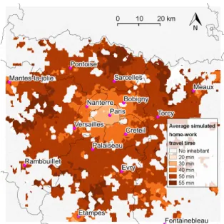
Figure4ashows a map of commuting times simulated by the model. As for commuting dis-tances, they mainly depend on the distance to major job centers. In total, average simulated (38
(a) An example of simulated excess commuting: sim-ulated fraction of the inhabitants who work inside Paris city.
(b) Comparison of average commuting distance as a function of households home location in the simula-tion and in data (Source: INSEE, French populasimula-tion census).
Figure 3: Excess commuting in the model and in data. Simulated average commuting distance is 9.5 km, to be compared with actual average commuting distance in Paris urban area which is 9.2 km (Source: INSEE, French population census).
(a) Simulated average home-work transport times (year 2008). This average is only computed for places in which the model simulates a non-zero urban popu-lation (other places appear in grey).
(b) Comparison of simulated and actual repartition of commuting times in the population, year 2008 (Source: INSEE, ENTD database).
Figure 4: Commuting transport times. Simulated average home-work transport time is 38 minutes, to be compared with actual average home-work transport time in Paris urban area which is 34 minutes (Source: INSEE, ENTD database).
min) and measured (34 min) commuting transport times in 2008 are very close (data source: IN-SEE, ENTD database).
The repartitions of commuting times in the population in simulation and in data also follow the same general pattern, with a large fraction of people with home-work transport times between 15 and 45 minutes (Fig. 4b). However, the simulation tends to underestimate both very short (less than 15 minutes) and very long (more than 60 minutes) trips. Several reasons may explain this: for instance, the logit function that we use to quantify population mixing may not be adequate for large variations from average behavior (the simulation is parameterized based on average values). Another explanation may be the fact that the model does not take into account mainly rural areas, in which live both people with extremely short (people in the farming sector living close to their fields) and extremely long commuting times (people living in rural areas but working in urban centers).
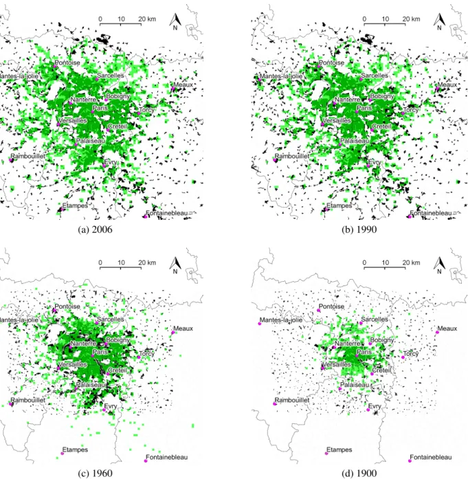
4.4.3. Urban area evolution
As can be seen on Fig.5a, the model reproduces well the current Paris urban area. Fig.5d, Fig. 5cand Fig.5bcompare simulated urban area with actual urbanized area, in 1900, 1960 and 1990, respectively. Because of the lack of data, we used the same transport network as in 2006 to do these three simulations, and the description of the city in 1900 is not as good as for the following years15. However, large-scale trends between 1900 and 2006 are well described, suggesting that the model captures the main determinants of city shape evolution.
5. Conclusion
Understanding households location choices and rent creation in a polycentric city is necessary if one wants to understand to what extent it is possible to act on commuting transport demand. There is a double challenge : one has to explain why households do not minimize their commuting distance, and one has to explain why households with different characteristics can live at the same location, even if rents are determined through a bidding process.
In the literature, it has been proposed that adding some qualitative mechanisms to traditional urban economics framework could address these issues. However, only a few of these mechanisms have actually been incorporated in this framework in a rigorous way. One reason comes from the mathematical and conceptual difficulties arising when trying to merge new mechanisms with Alonso’s bid-rent principle.
This is problematic, because it prevents a quantitative comparison of the importance of these mechanisms. These mechanisms are of very different nature, and understanding their respective influence and evolution over time for a given city is necessary of one want to be able to act on transport demand.
We have shown here a way to add to canonical urban economics models one of the mechanisms which had not been added previously, namely the existence of moving costs and housing-search imperfections. This new framework is analytically tractable, and leads to rent patterns similar to
15For instance, bus and tramway networks are not modeled, whereas they were of great importance at the beginning
(a) 2006 (b) 1990
(c) 1960 (d) 1900
Figure 5: Simulated urbanized area compared to actual urbanized area. Actual urban area appears in black (Source: IAU, MOS database), whereas model simulation appears in transparent green.
the patterns obtained in the canonical framework. However, everywhere in the city coexist people working in different job centers.
When calibrated, such a model appears able to reproduce main characteristics of commuting trip patterns in Paris urban area, as well as rent levels and population densities across the city. It is also able to reproduce the main tendencies of past Paris urban area evolution. This is a strong argument in favor of the leading importance of this mechanism on the existence of excess commuting, and of its leading role on overall city structure.
However, this conclusion will only be rigorously validated when the other mechanisms will be integrated into urban economic framework in a consistent way, and the resulting model calibrated on several cities.
Acknowledgment
The authors are grateful to Nicolas Coulombel, Tarik Tazdait and participants to North Ameri-can Regional Science Council (NARSC) 2014 conference, especially Haoying Wang, Harris Selod, Jacques-François Thisse for interesting discussions. Paolo Avner provided helpful comments. References
Aguiléra, A., Wenglenski, S., and Proulhac, L. (2009). Employment suburbanisation, reverse commuting and travel behaviour by residents of the central city in the paris metropolitan area. Transportation Research Part A: Policy and Practice, 43(7):685–691. 00049.
Ahlfeldt, G. (2011). If alonso was right: modeling accessibility and explaining the residential land gradient. Journal of Regional Science, 51(2):318–338. 00046.
Alonso, W. (1964). Location and land use: toward a general theory of land rent. Harvard University Press.
Anas, A. (1983). Discrete choice theory, information theory and the multinomial logit and gravity models. Trans-portation Research Part B: Methodological, 17(1):13–23. 00271.
Anas, A. (1990). Taste heterogeneity and urban spatial structure: the logit model and monocentric theory reconciled. Journal of Urban Economics, 28(3):318–335. 00055.
Anas, A. (2013). A summary of the applications to date of relu-tran, a microeconomic urban computable general equilibrium model. Environment and Planning B: Planning and Design, 40(6):959–970. 00002.
Anas, A., Arnott, R., and Small, K. A. (1998). Urban spatial structure. Journal of Economic Literature, 36(3):1426– 1464. 01229 ArticleType: research-article / Full publication date: Sep., 1998 / Copyright ? 1998 American Economic Association.
Anas, A. and Kim, I. (1996). General equilibrium models of polycentric urban land use with endogenous congestion and job agglomeration. Journal of Urban Economics, 40:232–256. 00206.
Anas, A. and Rhee, H.-J. (2006). Curbing excess sprawl with congestion tolls and urban boundaries. Regional Science and Urban Economics, 36(4):510–541. 00087.
Anas, A. and Rhee, H.-J. (2007). When are urban growth boundaries not second-best policies to congestion tolls? Journal of Urban Economics, 61(2):263–286. 00046.
Boiteux, M. and Baumstark, L. (2001). Transports: choix des investissements et coût des nuisances. Rapports du Commissariat Général du Plan, juin.
Boussauw, K., Neutens, T., and Witlox, F. (2011). Minimum commuting distance as a spatial characteristic in a non-monocentric urban system: The case of flanders: Minimum commuting distance in flanders. Papers in Regional Science, 90(1):47–65. 00021.
Brueckner, J. K. (2012). Lectures on Urban Economics. MIT Press, Cambridge, Mass. 00000.
Cao, X., Mokhtarian, P. L., and Handy, S. L. (2009). Examining the impacts of residential self-selection on travel behaviour: a focus on empirical findings. Transport Reviews, 29(3):359–395. 00206.
Castel, J. C. (2005). Les coûts de la ville dense ou étalée. Document de travail du CERTU.
Castel, J. C. (2007). Coûts immobiliers et arbitrages des opérateurs: un facteur explicatif de la ville diffuse. Annales de la recherche urbaine, 102(102).
Chang, J. S. (2006). Models of the relationship between transport and land-use: A review. Transport Reviews, 26(3):325–350. 00039.
Chang, J. S. and Mackett, R. L. (2006). A bi-level model of the relationship between transport and residential location. Transportation Research Part B: Methodological, 40(2):123–146. 00034.
Crane, R. (1996). The influence of uncertain job location on urban form and the journey to work. Journal of Urban Economics, 39(3):342–356. 00088.
Cropper, M. L. and Gordon, P. L. (1991). Wasteful commuting: a re-examination. Journal of Urban Economics, 29(1):2–13. 00115.
Dickerson, A., Hole, A. R., and Munford, L. A. (2014). The relationship between well-being and commuting revisited: Does the choice of methodology matter? Regional Science and Urban Economics, 49:321–329. 00000.
Echenique, M. H., Hargreaves, A. J., Mitchell, G., and Namdeo, A. (2012). Growing cities sustainably: does urban form really matter? Journal of the American Planning Association, 78(2):121–137. 00043.
Ellickson, B. (1981). An alternative test of the hedonic theory of housing markets. Journal of Urban Economics, 9(1):56–79. 00195.
Ewing, R. and Cervero, R. (2010). Travel and the built environment: a meta-analysis. Journal of the American Planning Association, 76(3):265–294. 00305.
Floch, J.-M. (2014). Des revenus élevés et en plus forte hausse dans les couronnes des grandes aires urbaines. INSEE références, INSEE.
Fujita, M. (1989). Urban Economic Theory: Land Use and City Size. Cambridge University Press, Cambridge [Cambridgeshire].
Gobillon, L., Selod, H., and Zenou, Y. (2007). The mechanisms of spatial mismatch. Urban Studies, 44(12):2401– 2427. 00203.
Hamilton, B. W. (1982). Wasteful commuting. Journal of Political Economy, 90(5):1035–51. 00420.
Hamilton, B. W. (1989). Wasteful commuting again. Journal of Political Economy, 97(6):1497–1504. 00126. Horner, M. W. (2008). ‘optimal’ accessibility landscapes? development of a new methodology for simulating and
assessing jobs–housing relationships in urban regions. Urban Studies, 45(8):1583–1602. 00018.
IEA, I. E. A. (2013). Policy Pathways: A Tale of Renewed Cities. Organization for Economic, Paris, France. 00003. IPCC (2014a). Chapter 8: Tranport. In IPCC, editor, Climate Change 2014: Mitigation of Climate Change:
Contri-bution of Working Group III to the Fifth Assessment Report of the IIntergovernmental Panel on Climate Change. Cambridge University Press, Cambridge. 00000.
IPCC (2014b). Climate Change 2014: Mitigation of Climate Change: Contribution of Working Group III to the Fifth Assessment Report of the IIntergovernmental Panel on Climate Change. Cambridge University Press, Cambridge. 00000.
Kennedy, C., Steinberger, J., Gasson, B., Hansen, Y., Hillman, T., Havranek, M., Pataki, D., Phdungsilp, A., Ra-maswami, A., and Mendez, G. V. (2009). Greenhouse gas emissions from global cities. Environmental Science & Technology, 43(19):7297–7302. 00170.
Kim, S. (1995). Excess commuting for two-worker households in the los angeles metropolitan area. Journal of Urban Economics, 38(2):166–182. 00069.
Lemoy, R., Raux, C., and Jensen, P. (2010). An agent-based model of residential patterns and social structure in urban areas. Cybergeo : European Journal of Geography. 00007.
Lemoy, R., Raux, C., Jensen, P., and others (2013). Polycentric city and multi-worker households: an agent-based microeconomic model. 00001.
Levinson, D. M. and Kumar, A. (1994). The rational locator: Why travel times have remained stable. Journal of the American Planning Association, 60(3):319–332. 00226.
Ma, K.-R. and Banister, D. (2006). Excess commuting: a critical review. Transport Reviews, 26(6):749–767. 00056. Ma, K.-R. and Banister, D. (2007). Urban spatial change and excess commuting. Environment and Planning A,
39(3):630. 00034.
Martinez, C., Javier, F., and Donoso, P. P. (2007). MUSSA II: A land use equilibrium model based on constrained idiosyncratic behavior of all agents in an auction market. In Transportation Research Board 86th Annual Meeting. 00008.
Martinez, F. J. (1992). The bid-choice land-use model: an integrated economic framework. Environment and Planning A, 24(6):871–885. 00132.
Martínez, F. J. and Henríquez, R. (2007). A random bidding and supply land use equilibrium model. Transportation Research Part B: Methodological, 41(6):632–651. 00045.
McMillen, D. P. (2001). Polycentric urban structure: The case of milwaukee. ECONOMIC PERSPECTIVES-FEDERAL RESERVE BANK OF CHICAGO, 25(2):15–27. 00047.
Metz, D. (2008). The myth of travel time saving. Transport Reviews, 28(3):321–336. 00126.
Mills, E. S. (1967). An aggregative model of resource allocation in a metropolitan area. The American Economic Review, 57(2):197–210.
Mokhtarian, P. L. and Chen, C. (2004). TTB or not TTB, that is the question: a review and analysis of the empirical literature on travel time (and money) budgets. Transportation Research Part A: Policy and Practice, 38(9):643–
675. 00178.
Muth, R. F. (1969). Cities and Housing; the Spatial Pattern of Urban Residential Land Use. University of Chicago Press, Chicago.
Muto, S. (2006). Estimation of the bid rent function with the usage decision model. Journal of Urban Economics, 60(1):33–49. 00012.
Newman, P. and Kenworthy, J. (1999). Sustainability and cities: overcoming automobile dependence. Island Press. 01681.
Ng, C. F. (2008). Commuting distances in a household location choice model with amenities. Journal of Urban Economics, 63(1):116–129. 00022.
O Kelly, M. E. and Lee, W. (2005). Disaggregate journey-to-work data: implications for excess commuting and jobs-housing balance. Environment and Planning A, 37(12):2233. 00051.
Osland, L. and Thorsen, I. (2008). Effects on housing prices of urban attraction and labor-market accessibility. Environment and planning. A, 40(10):2490. 00042.
Rhee, H.-J. (2008). Home-based telecommuting and commuting behavior. Journal of Urban Economics, 63(1):198– 216. 00010.
Rickwood, P., Glazebrook, G., and Searle, G. (2008). Urban structure and energy-a review. Urban policy and research, 26(1):57–81. 00060.
Roberts, J., Hodgson, R., and Dolan, P. (2011). "it’s driving her mad": Gender differences in the effects of commuting on psychological health. Journal of health economics, 30(5):1064–1076. 00027.
Schafer, A. (1998). The global demand for motorized mobility. Transportation Research Part A: Policy and Practice, 32(6):455–477. 00215.
Schafer, A. (2012). Introducing behavioral change in transportation into energy/economy/environment models. 00006. Schafer, A. and Victor, D. G. (2000). The future mobility of the world population. Transportation Research Part A:
Policy and Practice, 34(3):171–205. 00500.
Small, K. A. and Song, S. (1992). " wasteful" commuting: a resolution. 00197.
Song, S. (1995). Does generalizing density functions better explain urban commuting? some evidence from the los angeles region. Applied Economics Letters, 2(5):148–150. 00011.
Stutzer, A. and Frey, B. S. (2008). Stress that doesn’t pay: The commuting paradox*. The Scandinavian Journal of Economics, 110(2):339–366. 00000.
Thorsnes, P. (1997). Consistent estimates of the elasticity of substitution between land and non-land inputs in the production of housing. Journal of Urban Economics, 42(1):98–108.
Tscharaktschiew, S. and Hirte, G. (2010). How does the household structure shape the urban economy? Regional Science and Urban Economics, 40(6):498–516. 00009.
van Ommeren, J., Rietveld, P., and Nijkamp, P. (1997). Commuting: In search of jobs and residences. Journal of Urban Economics, 42(3):402–421. 00132.
Van Ommeren, J. and Van der Straaten, W. (2005). Identification of’wasteful commuting’using search theory. Tech-nical report, Tinbergen institute discussion paper. 00003.
Van Ommeren, J. N. and Van der Straaten, J. W. (2008). The effect of search imperfections on commuting behaviour: Evidence from employed and self-employed workers. Regional Science and Urban Economics, 38(2):127–147. 00018.
Viguié, V. (2012). Urban dynamics modelling, application to economic assessment of climate change. PhD thesis, CIRED, Université Paris Est, Paris, France. 00001.
Viguié, V. and Hallegatte, S. (2012). Trade–offs and synergies in urban climate policies. Nature Climate Change, 2(5):334–337. 00025.
Viguié, V. and Hallegatte, S. (2014). Urban infrastructure investment and rent-capture potentials. World Bank Policy Research Working Paper, (7067). 00000.
Viguié, V., Hallegatte, S., and Rozenberg, J. (2014). Downscaling long term socio–economic scenarios at city scale: A case study on paris. Technological Forecasting and Social Change. 00003.
Weinberg, D. H., Friedman, J., and Mayo, S. K. (1981). Intraurban residential mobility: The role of transactions costs, market imperfections, and household disequilibrium. Journal of Urban Economics, 9(3):332–348. 00159. Wheaton, W. C. (1990). Vacancy, search, and prices in a housing market matching model. Journal of Political
Economy, pages 1270–1292. 00475.
Wheaton, W. C. (2004). Commuting, congestion, and employment dispersal in cities with< i> mixed</i> land use. Journal of Urban Economics, 55(3):417–438. 00074.
White, M. J. (1988). Urban commuting journeys are not" wasteful". The journal of political economy, pages 1097– 1110. 00211.
Wrede, M. (2014). Continuous logit polycentric city model. SSRN Scholarly Paper ID 2390599, Social Science Research Network, Rochester, NY. 00000.
Zahavi, Y. and Talvitie, A. (1980). Regularities in travel time and money expenditures. Transportation research record, (750). 00219.
Zamparini, L. and Reggiani, A. (2007). Meta-analysis and the value of travel time savings: A transatlantic perspective in passenger transport. Networks and Spatial Economics, 7(4):377–396.
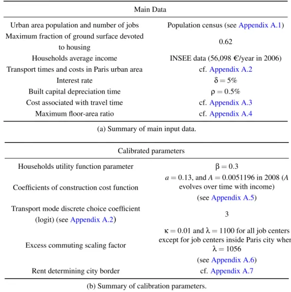
Main Data
Urban area population and number of jobs Population census (seeAppendix A.1) Maximum fraction of ground surface devoted
to housing 0.62
Households average income INSEE data (56,098 C/year in 2006) Transport times and costs in Paris urban area cf.Appendix A.2
Interest rate d = 5% Built capital depreciation time r = 0.5% Cost associated with travel time cf.Appendix A.3
Maximum floor-area ratio cf.Appendix A.4
(a) Summary of main input data. Calibrated parameters
Households utility function parameter b = 0.3 Coefficients of construction cost function
a = 0.13, and A = 0.0051196 in 2008 (A evolves over time with income)
(seeAppendix A.5) Transport mode discrete choice coefficient
(logit) (seeAppendix A.2) 3
Excess commuting scaling factor
k = 0.01 and l = 1100 for all job centers except for job centers inside Paris city where
l = 1056 (seeAppendix A.6) Rent determining city border cf.Appendix A.7
(b) Summary of calibration parameters.
Table A.1: Summary of main data and calibration parameters Appendix A. Data and coefficients
Tab. A.1presents the numerical data we used in our simulations. In absence of adequate data for some parameters, for instance construction costs, these parameters (“calibrated parameters”) have been calibrated on the structure of Paris in 2008.
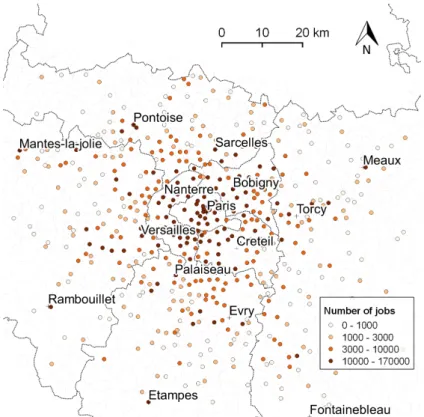
Appendix A.1. Job repartition
In the simulation, we consider 513 job centers (Fig. A.6). Job data is available at the “com-mune” scale (local administrative district). To choose the job centers, we have divided the simu-lation area into 4*4 km cells, and have considered that all jobs in these cells where located in the center of the commune of this cell with the biggest number of jobs. For computational efficiency, we have then discarded all cells with less than 300 jobs. Due to the large number of jobs involved, we have also considered each “arrondissement” of Paris to be a job center of its own.
Figure A.6: Job centers used in the simulation (the number of jobs is given for year 2007). The number of jobs is taken from French population census for years 1968, 1975, 1982, 1990, 1999 and 2007. A linear interpolation is used for the other years. Job repartition for years before 1968 was not available. We therefore supposed that, in 1900, jobs were only located inside Paris city. A linear interpolation is again used for years between 1900 and 1968.
The total number of jobs in these data does not play a role in the simulations. Indeed, to take into account the fact that labor force is only a part of all city inhabitants, we homogeneously rescale the number of jobs of job centers so that its sum over the city is equal to the number of households in the urban area, as given by the population census.16
Appendix A.2. Generalized transport prices
To compute generalized transport prices, we used data about walking times, actual transport times and prices in public transport (underground, regional trains and suburban trains) and private transport (during rush hours, for an average car). At each location, the generalized transport cost is computed for each transport mode, and a logit weighting is used to compute the modal shares17. In the simulations, changes in public and private transport prices lead therefore to modal shifts.
16 i.e. for each year, we multiply the number of jobs of each job center by a ratio equal to the total number of
households in the urban area divided by the total number of jobs.
17More rigorously, at each location, the logit weighting is computed on each price divided by the minimum price at