An analysis of finite elements for plate bending problems

An Analysis of Finite Elements for Plate

Bending Problems

by

Alexander G. Iosilevich

Moscow State Technical University, Russia (1994)

Submitted to the Department of Mechanical Engineering

in partial fulfillment of the requirements for the degree of

Master of Science in Mechanical Engineering

at the

MASSACHUSETTS INSTITUTE OF TECHNOLOGY

June 1996

@

Massachusetts Institute of Technology 1996

All rights reserved

/'? j,

Signature of Author.

...

Ipartment of Mechanical Engineering

June 1996

Certified by ... ...

...

Klaus-Jiirgen Bathe

Professor of Mechanical Engineering

e

& Supervisor

Accepted by ...

...

OF TECHNOLOGY

JUN

2

71996

Ain Ants Sonin

Chairman, Graduate Committee

Eng.

An Analysis of Finite Elements for Plate Bending

Problems

by

Alexander G. Iosilevich

Submitted to the Department of Mechanical Engineering on June 1996, in partial fulfillment of the

requirements for the degree of

Master of Science in Mechanical Engineering

Abstract

This thesis focuses on the inf-sup condition for Reissner-Mindlin plate bending finite elements. In general, one cannot analytically predict whether this funda-mental condition for stability and optimality is satisfied for a given mixed finite element discretization. Therefore, we develop a numerical test methodology to tackle this issue, and apply the tests to the standard displacement-based elements and the elements of the MITC family. Whereas the pure displacement-based ele-ments fail the tests, we find that the MITC eleele-ments pass them, which underlines the reliability of these elements for use in engineering practice.

Thesis Supervisor: Klaus-Jiirgen Bathe Title: Professor of Mechanical Engineering

Acknowledgements

I would like to express my sincere gratitude to my advisor, Professor Klaus-Jiirgen Bathe, for his invaluable guidance, enthusiasm, and encouragement through the course of this work.

I am also indebted to Professor Valery Svetlitsky and Professor Alexander Gouskov from Moscow State Technical University, who introduced me to the field of Applied Mechanics.

In addition, it is my pleasure to thank my collegues in the Finite Element Research Group at M.I.T., for their friendly support, invaluable discussions, and suggestions through the course of the research.

I would also like to thank ADINA R&D, Inc. for allowing me to use their proprietary software - ADINA, ADINA-IN, and ADINA-PLOT - during my work on this project.

Contents

2.1.1 Assumptions on the domain . . . . 2.1.2 Functional spaces. ... ... ... .

2.1.3 A simple example . ...

2.2 The problem statement and mathematical models. . . 2.3 RM plate bending model ...

2.3.1 Governing equations. Variational form... 2.3.2 Discrete variational problem.. . . . . 2.3.3 Modified variational problem . . . . .

2.4 Mixed interpolation. FEM with Lagrange multipliers. 2.4.1 Limit problem . ...

2.4.2 Optimality in F'. ...

2.4.3 Existence and uniqueness of the solution for Lagrange multipliers . . . . . 12 . . . . . 12 . . . . . 12 . . . . . 14 . . . . 17 . . . . . 19 . . . . 21 . . . . . 21 . . . . . 23 . . . . . 26 . . . . . 26 . . . . 26 . . . . 28 FEM with

3 MITC plate bending elements.

3.1 Design principles . . .. .. . .. .. .. .. .. ... .. . . . . ..

37

3.1.1 Preliminary considerations . . . . .

3.1.2 Stokes analogy. ...

3.1.3 Construction of the elements . . . . .

3.1.4 Justification. ... 3.2 The elements . ...

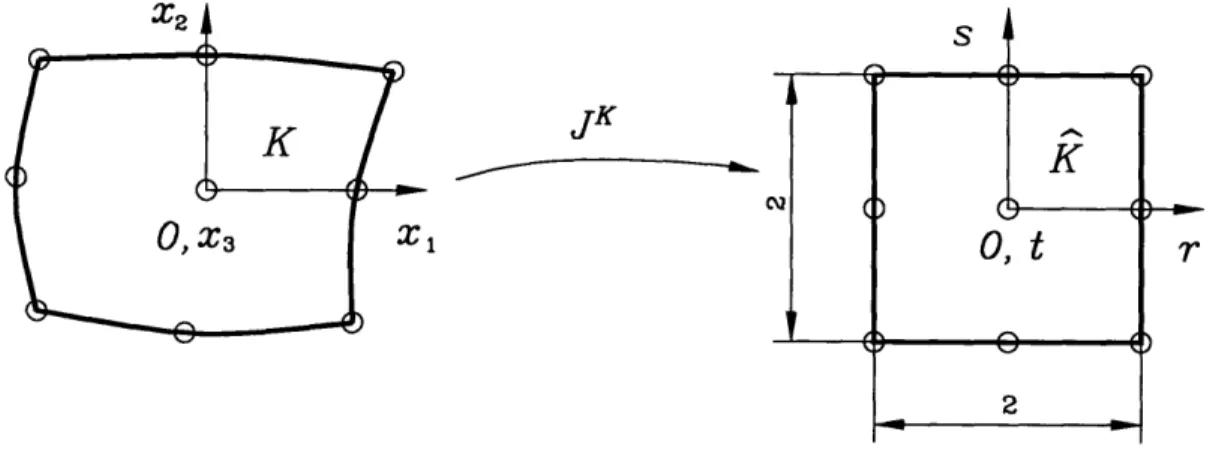
3.2.1 Reference element and covariant transformation. 3.2.2 Displacement-based finite elements . . . . .

3.2.3 MITC4 element. ... 3.2.4 MITC9 element. ... 3.2.5 Other elements ...

4 Numerical analysis.

4.1 Matrix computations ...

4.1.1 Eigenvalue decompositions. Generalized eigenvalue problems. 4.1.2 Vector and matrix norms. Basic inequalities . . . . 4.2 Analysis of the inf-sup condition . . . . .

4.2.1 _{Matrix form of the inf-sup condition in the F'-norm. .} 4.2.2 Discrete inf-sup condition in the L2_{-norm . . . . .}

4.2.3 Inf-sup test in the IF-norm . . . . .

4.2.4 From F, to F'. . ... 4.3 Num erical results ...

5 Conclusions. A Shear locking.

A.1 Cantilever plate under a uniform load . . . . .

A.2 Clamped square plate under a uniform load . . . . . B Inf-sup test in the F',-norm.

53 53 54 55 57 57 58 60 62 67 74 76 76 79 83 . . . . . 37 . . . . . 39 . . . . . 42 . . . . . 44 . . . . . 46 . . . . . 46 . . . . . 47 . . . . . 48 . . . . . 50 . . . . . 52

List of Figures

2-1 (A) - Domain with Lipschitz-continuous boundary; (B) -

Lipschitz-continuity is violated in the circled region. . ... 13

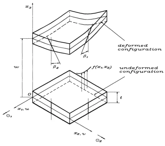
2-2 Displacement assumptions of the RM plate bending model... . 21

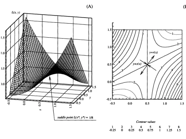
2-3 (A) - the saddle-point problem; (B) - contour plot of the saddle surface. ... 33

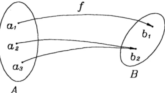
3-1 Surjective function. .... ... . .... .. ... . 45

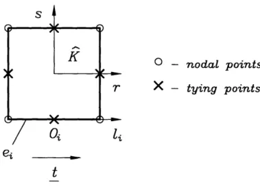
3-2 Covariant transformation of a general element... . . . 47

3-3 Tying procedure for the MITC4 element. . . . .. . . . . 50

4-1 Cantilever plate considered in the inf-sup test. Top view shows a typical mesh of four none-node elements. . ... . . 59

4-2 Inf-sup test of plate bending elements in the L2_{-norm (cantilever} plate). ... ... 60

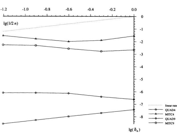
4-3 Inf-sup test of the plate elements in the Fi-norm (cantilever plate). 62 4-4 Behavior of 6, for quadrilateral plate bending elements (cantilever plate). ... 66

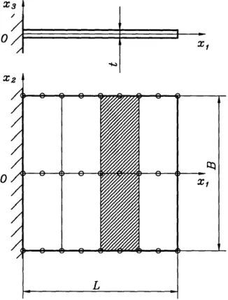
4-5 Clamped plate ... ... 68

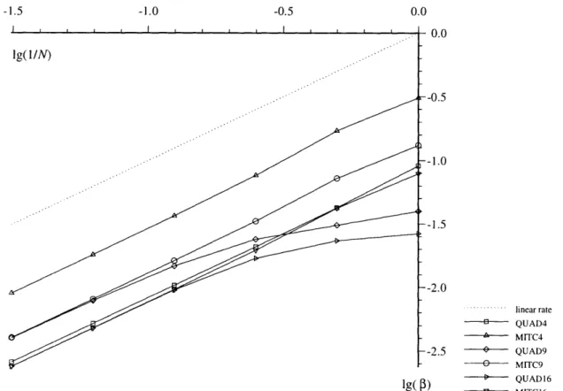
4-6 Uniform meshes used for the inf-sup test of the clamped plate case. 69 4-7 Inf-sup test of the quadrilateral plate bending elements in the F-~ norm (clamped plate case, uniform meshes). . ... 70

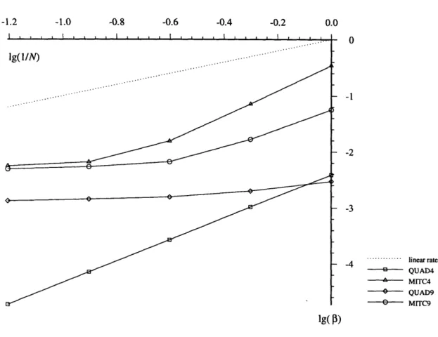
4-8 56-test of the quadrilateral plate bending elements (clamped plate case, uniform meshes). ... 71 4-9 Distorted meshes used for the inf-sup test of the clamped plate

probem . . . 72 4-10 Inf-sup test of the quadrilateral plate bending elements in the

rF-norm (clamped plate, distorted meshes). . ... 73 A-i Cantilever plate under a uniform load. . ... 76 A-2 Finite element solution (four-element meshes) for the cantilever

plate case. (A) - transverse displacement w, mm; (B) - rotation angle 0y; (C) -normal stress oa, MPa; (D) - shear stress a13, MPa. 78

A-3 Clamped plate under a uniform load. . ... 79 A-4 FE solution for the transverse displacement w, mm, (8-by-8

uni-form meshes for 4-node elements, 4-by-4 meshes for 9-node ele-ments) for the clamped plate case. (A) - QUAD4 element; (B) -MITC4 element; (C) - QUAD9 element; and (D) - MITC9 element. 81 A-5 FE solution for the transverse displacement w, mm, (8-by-8

dis-torted meshes for 4-node elements, 4-by-4 meshes for 9-node ele-ments) for the clamped plate. (A) -QUAD4 element; (B) -MITC4 element; (C) - QUAD9 element; and (D) - MITC9 element... . 82

List of Tables

A.1 Comparison of elements' performance in the norm IIWhII (cantilever

plate). ... 77

A.2 Comparison of elements' performance in the norm IIWhll (clamped plate case, uniform meshes, 8x8 meshes for four-node elements, 4 x 4 meshes for nine-node elements). . ... 80 A.3 Comparison of elements' performance in the norm I|whll (clamped

plate case, uniform meshes, 16 x 16 meshes for four-node elements, 8x8 meshes for nine-node elements). . ... 80 A.4 Comparison of elements' performance in the norm Ilwhll (clamped

plate case, distorted meshes, 8x8 meshes for four-node elements, 4 x4 meshes for nine-node elements). . ... 80 A.5 Comparison of elements' performance in the norm IIWhll (clamped

plate case, distorted meshes, 16 x 16 meshes for four-node elements, 8x8 meshes for nine-node elements). . ... 82

Chapter 1

Introduction.

1.1

Overview.

Finite element analysis of engineering problems in solid body mechanics often requires the use of plate bending elements. The design of such elements can be based on the Kirchhoff theory of plates. Then, because of the assumptions in this theory, the conforming finite element spaces are required to satisfy Cl-continuity. In the 1960's many Kirchhoff-theory-based conforming finite elements were proposed, among them the Clough and Tocher four-node quadrilateral element [21], the quadrilateral element based on the use of Hermitian functions by Bogner et al. [12], etc. Conforming plate elements were not only difficult to obtain, but also, the lower order elements turned out to be too stiff, resulting in displacements much less then the theoretical values. There were several attempts to use non-conforming elements, such as the nine-dof triangular element proposed by Bazeley et al. [11], but these elements often failed the patch test and even converged to incorrect results.

The subsequent research followed several different paths. Some researchers implemented elements based on alternative variational principles. One choice was to use the principle of complimentary potential energy, which gave rise to

so-called "equilibrium formulations" ([51], [37]). These methods partly suffered from non-uniqueness of displacement fields, which were obtained from integrating the strains.

Another popular approach, known as the hybrid stress method, was pioneered by Pian and Tong ([40]). It is based on the use of Lagrange multipliers, which force interelement equilibrium in a modified principle of complementary potential energy.

Later Tong [50] developed the displacement hybrid approach, based on a modified form of the principle of minimum potential energy.

In the 1970's the first elements appeared built on the basis of Mindlin plate theory and reduced integration schemes. The motivation for the use of Mindlin theory was that only Co-continuity of the shape functions is required. As well, the simple shape functions from plane elasticity could be used along with isopara-metric maps of distorted elements. This approach worked quite well for thick plates. However, as the thickness is decreased, the shear terms grow rapidly, in the limit resulting in zero displacements. This phenomenon was named (shear) locking.

To avoid shear locking, it becomes necessary either to impose the Kirchhoff compatibility condition directly as a constraint at discrete points or in the integral sense, or use some kind of numerical tricks (such as reduced integration) to avoid the unbounded growth of the shear energy part.

The latter direction was developed quite intensively in the 1970's ([53], [39]), while it was not realized that the use of reduced integration often distorts the results, and is not reliable to use in engineering practice.

The application of Lagrange multipliers to impose the Kirchoff constraint resulted in the development of mixed methods. These element families, if properly designed, have a strong mathematical basis (see, e.g., [18] and references therein) and are robust to changes in thickness.

Of course, this brief review does not pretend to cover all directions and trends 10

in the plate bending element design and research. In particular, we have not men-tioned "generalized equilibrium methods", "generalized displacement methods", and many others. For a much broader discussion we refer to the 1984 review article by Hrabok and Hrudey ([27]).

1.2

Thesis outline.

In Chapter 2 we start by covering some basic mathematical notions, which are abundantly used in the analysis of the finite element method. We define in a quite rigorous way the assumptions made, terminology used, and cite some general results dealing with associated functional spaces. Then we briefly cover existing mathematical models of the plate bending problem, and emphasize the basic assumptions and equations of the Reissner-Mindlin model. Finally we derive the mixed variational principle and show the necessary and sufficient conditions for existence, uniqueness, and stability of the solution.

Chapter 3 presents design principles and a mathematical analysis of the el-ements from the MITC (mixed interpolated tensorial components) family, and specifies the conditions reviewed in the second chapter for the problem under consideration.

Chapter 4 deals with numerical analysis of the elements, and provides the essential theory for tackling problems of the inf-sup type. There we develop a testing methodology, which allows to quantitatively analyze elements' "addic-tion" to locking behavior, and we apply these tests to the MITC elements and displacement-based elements.

Finally, Chapter 5 draws some conclusions and outlines possible extensions for further research.

Chapter 2

Basic notions.

2.1

Mathematical background.

This section summarizes some mathematical notions and definitions which are ex-tensively used in the mathematical analysis of the finite element method (FEM).

2.1.1

Assumptions on the domain.

The problem of consideration is posed in the domain Q E IRW, n = 2, with sufficiently smooth boundary O0f. Let us formally define what is usually meant by the "sufficiently smooth boundary" ([22]) in the finite element literature.

An open set f E IRn has a Lipschitz-continuous boundary if there exist con-stants a, 3 > 0, a number of local reference coordinate systems {QO E IRn_{, x}} and local maps a3 _{() , j = 1..J, Lipschitz-continuous}1 _{on their respective domains}

1_{A real-valued function f of a single real variable x, defined over a domain Q}

is Lipschitz-continuous if:

If

f

X21

of

definition

{

JRn-

1

_.Ix:

_l

_<

_{u), such that}

j=1

{xi : aj (ji) < xi < a3 (,Kj) +

L,

ai

: a3 (ji) - # < x3 <a < (ji), jx1i <al E Q,

where f stands Geometrical

for the complement of Q, (T = IR" \ Q).

interpretation of this condition for f E IR2 is shown in Fig. 2-1.

e2

ey

Figure 2-1: (A) - Domain with Lipschitz-continuous boundary; (B) - Lipschitz-continuity is violated in the circled region.

The definition above allows to consider all commonly encountered shapes, though eliminating some special cases, such as domains with cusped corners, cracks, etc., which require special treatments (see e.g. Chap. 8 of [46]).

When all of the maps a' (.), j = 1..J are linear, we have a special case, that

is, Q is a convex polygon.

If an open set Q is connected and there exists a finite number of convex polygons Qk, such that Q = (n k , then Q is called a polygon.

We will always assume that one of the following properties hold:

* Q has a Lipschitz-continuous boundary; or

* Q is a polygon.

In either case Q is bounded, that is, there exists a constant M :

IIv

Q (in other words, any vector drawn inside Q has a finite length - i.e., semiinfinite bodies that often appear in the elasticity do not satisfy this condition).

2.1.2

Functional spaces.

In this section we introduce the basic functional spaces that will enable us to make variational statements.

A real-valued function f is said to be Lebesgue measurable on Q if for every real number A, the subset w :

fl,

Firstly, for LP (Q) ,p E [1, 00), we set

1

LP (Q) = v E M () I P

d

<vIdI

,Ivjd

where M (Q) stands for the space of functions, Lebesgue measurable over domain

1

2_{f (X) =}

- is an example of a function measurable on the interval Q2 = [-1; 1]. Although

f (x) is not bounded on the subset w = {z = 0}, the measure (length) of w certainly is well-defined, and equals to zero. Examples of nonmeasurable functions are more difficult to find, although they certainly exist (see, i.e., [30]).

Remark. All finite element spaces are constructed over the space M (Q).

This guarantees that integrals of the functions under consideration are well-defined, or, roughly speaking, functions are not too irregular (i.e., functions that have infinitely many singularities are not admissible). For example, such cases as an infinite stress in the semiinfinite body are ruled out by construction. LO

In future, we will deal with one particular member of the family, namely, the space of square-integrable functions, L2 (Q), with the scalar product given by

(u, v)L2() =

uv

dQ.

The operation (-, ) would be considered as the L2 (Q)-inner product by default. Secondly, we introduce the Hilbertian Sobolev spaces (in future referred to simply as Sobolev spaces) with an integer index Hk (Q):

Hk (Q) = v E L2

() , Dcv E L2 _(q),

Ia_ < k},

where

alvln

DOv

.Oxin,

Ia!

1 n i=1

equipped with the following inner product, seminorm, and norm: k

(u,

V)Hk() =1

E

D u Day dQ,

72 k'd=2

IVlHk(-)

|Da

L

()

IIDv=O

-The following inequality holds. Let a real valued function f (xl, ... , xn) e Hfk (Q), with k > n/2, and let f be continuous, then

This inequality is often referred to as Sobolev inequality.

Example.

To demonstrate the implications of the inequality (2.2), consider a function

f (x, y) = f (r) = ig (lg (r)),

defined over a domain = r, r = x2 + x 22r < 1/2. One can show that

f E

JIfIIH1(0)

C1

Q. Indeed, we have that f -- oc, and the inequality (2.2) clearly does not hold.

r-+O

The family of functional spaces defined below corresponds to the homogeneous boundary conditions on O0 (homogeneous spaces)

Hk (Q) = {v E Hk _{(Q), DvlIan = 0,}

l•a

When the domain Qt is bounded, we have the following norm equivalence, referred to as Poincare'-Friedrichs inequality [22]:

Co (A ) vIIVHk(Q) • IVHk(o) c1

(C )

For the further analysis we also need spaces of functionals L£ Hk (Q) -- IR, defined over the Sobolev spaces (topological duals, or so called negative Sobolev

spaces): H- k _{(Q) = (Hk (a)). For a pair}

_(f,

_K

for a Sobolev space, we define a duality pairing on IC' x

KC

The corresponding dual norm is

If

EKIIl•,

= sup

The following result is referred to as the Riesz Representation Theorem:

Let IC be a Hilbert space, and f E IC' be a continuous linear fuctional on 1C. Then there exist a unique uo E IC, such that f (u) = (uo, u) , Vu E 1.

Moreover, I|f ll, = IIU01o1C

The proof of the theorem can be found, e.g., in [38], [52].

In case 9 = {x : x E ]x; 2[ C IR}, we have the following mapping K [38],

K: Hk (Q)

H-k(Q),

Finally, we state the following inclusion property of the Sobolev spaces

Hm (Q) C Hm-1 (Q) C ... C Ho (Q) C ... C H-m+1 (Q) C H-m () , V m > 0.

(2.5)

For a general study of the Sobolev spaces we refer to [1].

2.1.3

A simple example.

Consider a truss of length L (Q = {x : x E ]0; L[}) fixed at the end points x = 0, x = L, under the action of a distributed load f (x). Let the deflection of the truss be w (x) : w (x) E Hl (Q) (clearly, this must be the case of a real physical system), and presume that f is square-integrable over Q. Noting that f (x) E L

(

as

L

(f

fw

dx,

which has a meaning of the work done by external forces. Actually, to obtain a finite number as a result of the duality, we do not have to enforce w to be in H1;

indeed, the L2 regularity is sufficient for the functional in (2.6) to make sense (to give a finite number).

Now we consider the case f (x) = 6 (x - L/2), that is f (x) E H-' (Q). In

this case, to obtain a finite scalar number after the integration, w (x) must be continuous on Q); we have to use the fact that w (x) E H1 (Q), and the duality pairing defined above still works.

The norm of f can be calculated as

v

(L/2)

by

(2.2)

=,llHmax << C, - -HI() IIVIIHI()

which is finite, according to Sobolev's inequality.

To demonstrate a Riesz representation of f (x) in Ha (Q), we will find a linear operator K, such that every v (x) E Hl (Q) has a unique image Kv (x) in H- 1 (9). Using formula (2.4), we can simply construct this operator as K = + 1.

dZ₂

Since H- 1 (Q) contains Hl (Q) as well as singular functions of type f (x), the operator K can be understood as a superposition of 6-function-like distributions, given by the first term, and H0 (9) represented by the unitary transformation. To find an element v1 (x) E HJ (Q) that is the Riesz representation of f, we have

to solve a differential equation

d2vf (x)

Kvf

(x)=

-

+v (x)

= f

(x).

sinh (-L/2) sinh (x) The solution is vf (x) = -H (x - L/2) sinh (x - L/2)+ sinh (x)

Re-sinh (-L)

L dudv\

calling that the inner product in H1 (Q) is given by (u, v)H1(0)

f

one can check that indeed,

fw dx = w (L/2) = (v),w)H, VwE H1 (Q) .f

0

2.2

The problem statement and mathematical

models.

Consider a three-dimensional linear elastic body B that, in the absence of external loading, occupies the region

S= {X

= (x

,

,

) E

(X

, X

) E Q, X

E -2,t

[

where Q E IR2 is a bounded smooth domain with boundary 0Q, and t > 0 is "relatively small" with respect to diam (Q).

By the exact solution of a linear elastic plate bending problem, we understand the solution of the three-dimensional linear elasticity problem of deformation of the body B under the action of a transverse load

f=

displacement vector, stress tensor, and strain tensor, respectively, we have the following stress-strain relations given by Hooke's law:

011 022 033 (12 "23 0'13 A + 2y A A A A +2 2 A A A A

+

Ev E

where A = v)and ( = are the Lame constants (elements (1 + v) (1 - 2v) 2(1 + v)

not shown are zeroes).

By the plate bending model we mean a two-dimensional boundary value prob-lem with a solution, which approximates the exact solution of the plate bending problem.

The following two models are extensively used in engineering practice (see

[26], [3] for the comparison of the models and references therein):

* The Kirchhoff model (see, e.g., [48]) is based on the assumption that all

out-of-plane components of the stress tensor are negligible (we set the com-ponents ai3, i = 1..3, to be zero). Geometrically this implies that a straight

element normal to the midsurface remains straight and normal after defor-mations. This model provides a good approximation for the plate bending problem only for thin plates, that is, in the case t < diam (Q). The most important disadvantage of the model is that the strains are calculated as corresponding second derivatives of the state variable w (transverse dis-placement). In terms of finite elements, it requires C' continuity of the interpolation functions. Moreover, the model suffers from the inherent lim-itations, such as paradoxical artificial reaction forces on the corners of polyg-onal domains, and difficulties in imposing natural boundary conditions.

* The Reissner-Mindlin model (RM) ([43], [361) uses the condition a3 3 <K

all, 22 (that is, we set only a33 to be zero, leaving shear strains for the

consideration), and therefore, is closer to the original 3D problem. The basic hypothesis of this model is that a straight line normal to the undeformed plate surface Q remains straight but not necessarily normal during the deformation (see Fig. 2-2). Finite elements based on this RM model need to have only Co continuity of the interpolating spaces. Moreover, this approach is far more flexible in allowing to model many types of boundary conditions without significant difficulties (see [26]).

2.3

RM plate bending model.

This section describes the basic equations and specific difficulties associated with the RM plate bending model. The more precise analysis can be found in [48] and [23].

2.3.1

Governing equations. Variational form.

fo-rmre c n figturctionL d eforvnme d I~nfigura tio0 T 0, 02

Figure 2-2: Displacement assumptions of the RM plate bending model. The equations governing the model are [6]:

1. Displacements (assumed to be small)

Ul = -X 301; U2 = -X 3/3; U3 = w, (2.7)

where /1, #2, and w are the scalar functions of the in-plane vector coordinate

2• = (x1

,

2. Strains (linear part of the strain tensor)

11 = -x~₃ l,'1;

622

1 1 2 (2.8)

E13

2

(W,1

-

01);

2

(,

),

8F

where "F,i" denotes the partial derivative ₉

xi

3. Stresses (isotropic elastic material assumption)

E E

1- -

V

11); 033 = 0;

O12 = 2Ge12; '13 = 2GE13; o23 = 2GE23,

(2.9)

E

where G stands for the shear modulus, G =

2(1 + v)

4. The variational form as a starting point for a finite element analysis is formulated within the principle of minimal potential energy [28]. For the case of a clamped plate (the treatment of other types of boundary conditions is also possible, see [26]), we have the following minimization problem

Find u = (, w) V = B x W = [H1 (Q)]2 x H1 (Q) such that

=() 1 1t 2

arg min A (v,

where a (-, ) is a symmetric bilinear form defined as

t13

[(1- )

V)

-)

() +L"

('• -) (q)1

( 92

;

S(q_) is the linear strain operator:

S(/)

e 0

V= e- + e2;

89l-

-2;

(-, ) is the L2 (Q)-inner product;

Et3

D = _{stands for the flexural rigidity of the plate; and}

12(1 -

v2)

k is the shear correction factor that accounts for the nonuniformity of the

shear strain distribution through the plate thickness, usually k = 5/6. Note that for a finite fixed thickness t we have, expanding the bilinear forms and collecting the corresponding terms,

Gk

A (v,v) = a (, -)

+

c

Ilvl,-c(

2

11',

I1•1,), (2.11)

that is, A (v, v) is an elliptic bilinear form (the constant C in the inequality above depends on thickness and material properties of the plate).

The minimization problem (2.10) can be equivalently represented in the

vari-ational form:

Find u = (/, w) E V = B x W = [H1 (Q)]2 x Hl1 (Q) such that (2.12)

Gk 1

77)

_{+ - (VW - V• - y) = -is,}

_{U,(0,. _}

₎

_{E V,}

2.3.2

Discrete variational problem.

Typically one cannot find an analytical solution to (2.12). The usual way to proceed is to introduce a finite-dimensional problem which approximates the given one.

Let us choose a discrete space Vh = Bh X Wh C V, where Bh C B, and

Wh C W; thus we are restricted to using a conforming approximation.

Following the Rayleigh-Ritz procedure, we obtain the corresponding discrete minimization problem over the space Vh

Find Uh = (h, h) E IV = Bh X Wh, such that

u

=arg

min

1

1

(2.13)

MA

=arg

mm

-A(vhs h)-

, h)}.

_Vh=(r2h4)Eh h V h

2

t3

Let us rewrite the minimization problem (2.13) in the discrete variational form. For the following analysis, let us rescale the loading term f as f = t3g, with g

independent of plate thickness t. Then in case of finite t we have the following

discrete variational problem

Find u = ( wh) E Vh = Bh X Wh, such that

a _(7h'h h _--h) h -- = (g9,) VV h - (h' h) E Vh)

Gk 1 Gk

As t -0, wehavethat a , 17 t2 withi t2 = c0. Although the thickness may be very small, the energy of deformation still remains finite. To keep it finite, we must have that the shear strain contribution to the total po-tential vanishes, that is (Vwh -'h' •VG h - h) = 0 for all (h' h) E Vh. Clearly, this is nothing else, but the integral form of the celebrated Kirchhoff constraint

Vw = #. (2.14)

Equation (2.14) implies that in the limit case, the RM model must degen-erate to satisfy conditions on the stress-strain state, described by the Kirchhoff hypothesis. Thus, as we approach the limit case, the finite element solution is

more and more enforced to satisfy the Kirchhoff constraint. Consequently, the number of "conforming" (which can represent the Kirchhoff hypothesis (2.14)) trial functions in the discrete space Vh may get severely restricted, and this can result in partial or even total loss of convergence properties of the finite element approximation. This phenomenon is known in the literature as (shear) locking (see, e.g. [6], [47]).

Another difficulty for the numerical solution is due to the existence of bound-ary layers for various types of boundbound-ary conditions ([3], [44]).

General approaches.

There are two general approaches to circumvent the problem of locking described above. The first type of methods is based on the standard variational formulation, and uses convergence properties of higher order FE spaces (so-called p-version and certain higher-order h-versions [4]).

The other approach is to modify the variational formulation, and therefore, come to a different finite element formulation. The reasons for that treatment are:

* Difficulty to construct low-order finite element spaces, satisfying the con-straint (2.14) exactly;

* Possibility to introduce variables that have a certain physical interpretation. Those ideas are used in mixed and hybrid FEM (some other approaches, based on modifications of the variational form, such as reduced integration [35] and

penalty formulations are also well known in the literature). For some examples of

hybrid plate bending elements we refer to a recent paper [31], while some mixed finite elements would be the subject of the following discussion.

2.3.3

Modified variational problem.

The general guideline is to replace the Kirchhoff constraint by a weaker form, introducing a reduction operator Rh into the variational statement:

a1(h'7h) + Gk (Rh (Vwh -h),Rh (Vch ) ( (2.15)

Thus, choosing Rh = I, we have the standard FEM; if the reduction is based

on inaccurate numerical quadratures in evaluating the shear strain energy, we in essence use the idea of selective or reduced integration (if we treat distorted ele-ments by reduced integration, the operator Rh may become highly nonlinear, and could hardly be found in closed form). In the following, we will consider the case of mixed interpolation, where the shear stress is first approximated independently and then eliminated from the system.

Clearly, the choice of Rh in (2.15) is crucial: it should weaken the constraint (2.14) sufficiently, so that the FE spaces would retain their approximation prop-erties, while on the other hand, it should not weaken it too much, since otherwise the consistency error may become too large (that is, our solution will be far from the real one), or even the solvability conditions may be violated.

2.4

Mixed interpolation. FEM with Lagrange

multipliers.

2.4.1

Limit problem.

Before we proceed with mixed interpolation, let us define the shear stress in the plate and its discrete approximation as

Considering the variational problem (2.12), we note that for a finite thickness t, the fact that Vw E VW C [L2 (f)] 2, VWh E VWh C VW, implies that both

the shear stresses and their discrete version are sufficiently smooth (y E

g

[L2 (Q)]2, '~h E 9h C !). Noting that all linear operators defined on L2 (Q) are indeed in L2 (Q) (that is, [L2 (Q)]' = L2 (9) 3), we can represent equation (2.16) in the integral form as

(

Gk

(VW

V;

E

g.

This allows us to rewrite the variational problem (2.12) as

Find

u

=

(3,

w) E V = B x W = [Hd

(Q)]2

x Hl (Q), yE

9,

such that

[

)

+ (7,V

- 1-)

=(g,)

Gkt2

-

-

However, as we approach the limit case, t

-the L2-norm, that is

Vv _{= (YI 0 E V7}

(2.17)

0, we loose the regularity of y in

S1/2

Gk

(V2d

1/2

-- 00.

This suggests that we should look for the space for shears among the negative Sobolev spaces, as in the example in section (2.1.3), and the appropriate space

VA' would be the smallest one, in which the corresponding norm is finite, that is

3_{Namely, consider a function f E [L}2 _{(Q2)]'. We have}

ll[L ( )] -- Lsup (',v }[L2(Q)]'XL2( - s (,v)

v EIL[2(SI)() S V4 = IIVIIL2(0) vEL2(n),,O '/(7v)

= f) = IIAIIL2(l)

11211,, < c. Ideally, the constant appearing on the r.h.s. of this inequality should

not depend on the plate thickness t, though it is neither sufficient nor necessary for the bound to exist. In the following section we will show that the normed space F' = H-` (div; Q) satisfies the requirements given above, and

H-' (div; Q) = (_ e [H-' (2)12 , V y E H- 1

()

(2.18)

H-1 (div;) = 2 H-1(0) I VlH-1 (Q)

Therefore, when t approaches zero, we are able to pose the following limit problem:

Findu = (,w) E V = B x W = [H (Q)]2 _{x Ho (Q}) _and

7o e F' = H-1 (div; Q), such that

(2.19)

a (ýo 0)

+

(-o,

_

77) = (g,)

VV

E V)

(Vwo -P0,) =0

VE '

2.4.2

Optimality in F'.

Here we cite the result from the original paper [7], which explicitly shows the op-timality of the norm in H-1 (div; Q) (opop-timality is obtained in the sense that the norm of the shears in that space is finite and bounded by a constant independent of the plate thickness).

Theorem 1. We have

1(tj

<

c independent of t.

(2.20)

Proof.

1. For a finite but small t we have the following bound for the solution of

(2.17):

I v + t2 (t)2 c independent of t, (2.21) 28

where

•ji(2

1~1

+

II

2. By the Riesz Representation Theorem, we have that there exists a unique X E

r: (__(t),

x)

2(t

I

x e

(2.22)

Ky=xsup

,where

Ox

3. Choose 0 E B such that

V 0 = 01,1 + 02,2= X1,2 - X2,1 = - rot X,

II0|HI(o) l C

c

rt

X

.)

(2.23)

(2.24)

By definition of Ho (rot; 9), rds - =f rot X d = 0 =

which guarantees that such 0 can always be found as a

V.0dQ = 0,

solution to the well-known potential problem (e.g., Ch. 1, Sec. 2.1 of [33]).

4. Set 71 = (-02,

01).

rot rl = 02,2 + 01,1 =

V

and from

(2.24),

using I

rot

XIL

₍₍₎

jX<

_

_{we obtain}

IIIIH1(,)

10)

lH,(0)

lXl

(2.25)

5. Take

E HU1 (A) : = A-' (V + V -7).

(Note that both V - X and V - 7 lie in H-1_(Q)).Then

IIH(Q)) • C1 V

_{_+}

_,H.-)

_•

_<c

_(IIXl,

_{+ 1±_,11,)}

<CX _(xlLI() 2_{(QT) + I~IIIH1(I}-

)

o

*,

1=V

D -7

Moreover, using (2.25) in the form4

rot x = _{rot (Vý - Y)}

we obtain a system of PDE's (2.29-2.30) with a boundary condition, given by X -r = 0 on dO, which leads to the solution

(2.31)

From equations (2.26) and (2.28)

(1!l

III

)< c Xl

7. From part 2 we have that

[I__(ct)

r'

I

(

)

-

< C (jjijjj() + R (g,)) :5- C IIX1

4Here we invoked the equality rot Vcp = V x Vip = 0 for any scalar function p.

(2.27) CIIXII'

(2.28)

,.

which immediately implies (2.20). OE

Remark. In part 6 of the proof, we have shown that for all X in F, it is always

possible to find a pair (y, ý) in V, such that (2.31) and (2.32) hold, that is, the map B, : V - F, By = V77 - = X E is surjective (we will use this result

later). Clearly, the destination space will not change if we multiply the result

Gk

of the map B, by a finite constant, say, Gk , with t # 0 being a finite number. Now, we have identified that the subspace

g

2.4.3

Existence and uniqueness of the solution for FEM

with Lagrange multipliers.

The variational form (2.19), in fact, represents a typical case of the well-studied saddle-point optimization problem of the Lagrangian functional:

(u,Y) = inf sup L (v, ), where

(2.33)

,

(K,

x)=

{a

(KK) +

b(jv)

-

_(9q,)V'XV

-(see the original papers [13], [2], and a broad discussion in [18]). In this form _ stands for Lagrange multipliers associated with constraint (2.14), which have a physical meaning of shear stresses in the plate.

Remark. The equivalence of the Lagrangian formulation to the problem (2.19) can be shown, if we evoke the necessary conditions for stationarity of

£

(v, _) at the point

(1,

7), taking q = 0:

a (u, ) + b (21,) - (g, v)vxv = 0 V e V;

Here we present a brief discussion on the conditions for existence and unique-ness of the FEM solution in the problems of optimization of a quadratic functional under a linear constraint (2.33) (in our case the functional is given by (2.10), and the corresponding constraint is given by (2.14)).

Example. Saddle-point problem.

In this example we will consider a simpler problem. Assume that we are

1

supposed to find J* =min J (x) = -z 2. _{Trivially, J* = J - = To proceed}

X=1 2 2 8

with Lagrange method, we introduce a Lagrange multiplier y and Lagrangian

L (x, y) = J (x) - y x - ). Invoking stationarity conditions, we have

aL (x, y) x* 1 0 1

L

(xy

,y*) =

- y* =

o

y* = z* =

ay

2 2'

and min L (x, y) = L 1 1 - J*. The functional is shown in the Fig. 2-3.

Xy

(' 2

8

We thus have a saddle point at (x*, y*), such that L (x, r (x)) • L (x*, y*) <

L (x, s (x)), where r (x) and s (x) are the equations describing the unstable and

stable manifold of the saddle surface respectively. This problem is equivalent to min sup L (x, y) . To show the equivalence:

00,

i

sup L (x, y)= 2 1

(A) (B) Il ,'1 1.5 1.0 ).5 ).0 -0.5 0.0 0.5 1.0 1.5 Contour values 1 2 3 4 5 6 7 8 -0.25 0 0.25 0.5 0.75 1 1.25 1.5

Figure 2-3: (A) - the saddle-point problem; (B) - contour plot of the saddle surface.

1

min sup L (x, y) =min J (x)= -. O

x y x 8

The bilinear form a (-, -) defines a symmetric linear operator A : V -- V',

such that a (y,

v)

(Au,v),,xv

(uy,Av)v

operator associated with the bilinear form b

(-,),

BT F' -~ V'

BT

F' V'

B _V

Then

b(c,v) = (S - 7)=(S By (V- q))r'xr xV = (B 7 - 7)V'xV

and now we can rewrite the original problem (2.33) in the operator form:

Au+B

Bu =_q E r.

Moreover, let us denote the null space of B, as Ker (B,), and the range of B, as R (B,). Then we have the following very intuitive result that follows directly from the Lax-Milgram theorem [22].

Proposition 1. Let q E 7 (B,) and the bilinear form a (-, .) be elliptic on

Ker (B,), namely

3 ao > 0 such that a (v, v) > cio

IIvll

Then there exists a unique u E V, such that

a (,v) = (g,vy v Vv E Ker (B,), and

(2.35)

b S,11=(i7

,. ,

V

Ir'F

For the proof we refer to [18].

Proposition 1 implies that if the first component of solution, u, exists, it is unique. Condition (2.34) states the restrictions that we have to impose on the reduction operator Rh in (2.15) to obtain a unique u (a number of reduced-integrated elements violating this condition were proposed in earlier publications on the subject, see e.g., [29]).

Now we turn to the problem of finding the Lagrange multipliers, y. For this we have to make the following restrictions on B,, namely, we require R (B,) to

be closed in F.

Remark. Closed range operators. The concept of a closed range operator is a generalization of the idea of a bounded linear function. Moreover, the Closed

Graph Theorem states that if the range of an operator R (f), f : A -- B, where A and B are some Sobolev spaces, is closed in B, then f is continuous on its

domain D (f) = A. OE

Now we can apply results of Banach's closed range theorem: Proposition 2. The following statements are equivalent: (i) 1 (B,) is closed in F;

(ii) 7 (BT) is closed in V';

(iii) 3 k0 > 0 such that V qE R(By), 3 vq E V:

(iv) 3 ko > 0 such that Vg E R (BT), 3 Er':

BRyf 9 g,

2ff11

1r4'1.

For the proof of (i)-(iv) we refer to [5].

Remark. Basically, the closed range theorem is the straightforward extension of the closed graph theorem mentioned above. The most valuable addition to the continuity of B, (which is implied by (i) according to the closed graph theorem, and equivalent to saying (iii)), is the dual result for BT. EO

Now we can clearly define the norm over V' using duality arguments:

I sup I

and substituting this into equation (iv), we obtain the inf-sup condition as follows:

I

(BVxV/V'x V1

l llv

sup

sup

E

(2.36)

_

OsupIY>o

,7

Now we can summarize the results of propositions 1 and 2.

Proposition 3. Let the continuous bilinear form a (-, -) be elliptic on Ker (B,)

(that is, (2.34) holds). Moreover, let us suppose that the range of the formal op-erator associated with the bilinear form b (., -) is closed in F. Then there exists a solution to the problem of type (2.33) for any g E V' and q E 7 (B,).

Proof. Let q •R (B,) and u be the unique solution of the auxiliary problem (2.35). We need to show that if 7 (B,) is closed in F, then for all g E 7 (BT)

there exists 7 E F', such that (y, ) is the solution for (2.33).

Consider the linear functional on V: L (v) E R (BT) C V' :

L (v) = -a (., +v)+

(g,

V',xV

Firstly, take vo E Ker (By); clearly, by (2.35), L (0o) = 0 V v0 E Ker (B,), so

we indeed have a solution for that case.

Next, if v 0 Ker (By) then by (ii) in Proposition 2, the 7 (B T) is closed in

V'; this implies (by (iv) in Proposition 2) that there exists y E F', such that

L (p)

_{= b (Y,}

_{7v) .}

Remark. It could be shown that the inf-sup condition (2.36) along with the ellipticity condition (2.34) represent sufficient and necessary conditions not only for existence and uniqueness but also for optimality of the solution for the saddle-problem optimization (2.33) (see e.g. Theorem 1.1 in [18] and a broad discussion in [14]). The deeper insight into the physical meaning of the inf-sup condition can be found in [6]. o

Chapter 3

MITC plate bending elements.

3.1

Design principles.

In this section we present the design principles for the MITC family of plate bending elements, based on the RM-model and mixed interpolation. These results are adopted from original papers [15], [8].

3.1.1

Preliminary considerations.

For the further analysis we shall consider the limit, and therefore, most severe case t = 0, presuming, that if our finite element discretization provides a good solution for that case, then the elements will not lock in any other case.

Summarizing the results of the previous chapter, in the limit t = 0 we face the following modified discrete variational problem:

Find uh = (hWh) e Vh = Bh X Wh and --h E h = Rh (Bh U VWh) , such that

a

(1h'

_h)

+

(2h'

Rh (v

-

)) =

(g,7 )

VVh

= (1,h7,]

)

e

Vh,

hRh (V -

h)) =

Xh E

h(3.1)

Moreover, as we have shown in section 2.4.3, we obtain a unique solution for Uh, if

3 ao > O: a (h' ,rh) - _{QO I1hlI V VPh = (rh, Ih)}

_E

and a unique and stable solution for 7_h if

3 ko

> 0

:

f

sup

Rh

(

h- ))

>

o,

(3.3)

where

IIX

,= sup

=-')rx

sup (Xh, 2_

Clearly, the choice of the functional spaces Vh, Gh, and the reduction operator

Rh is of great importance, and determines existence and behavior of the solution. Let us make the first step that puts some structure on Rh and is crucial for the formulation of the elements. We choose Rh : Vh -- h to satisfy

(Rh - I) V~h = _0 V h E Wh, (3.4)

9c C

0 :

11R

NHI ( < C

Jc

h

HI (0)

(3.5)

where Gh - Fh is a subspace of the functional space F introduced in Section 2.4.2.

Remark. Condition (3.5) just enforces the continuity of the operator, and is quite natural due to the physics of the problem, while (3.4) is a rather strict condition which implies that we shall use the standard interpolation for the gra-dient of the transverse displacement field. This condition is sufficient, but not necessary to allow us to use the "energy-type" seminorm, defined on V by

as a norm, and thus, to be sure that the property (3.2) holds. Another possible condition would be, for instance (see [41]),

RhVGh = 0 'hG = 0

Vh E Wh. O

In the limit case our approximate solution should satisfy the Kirchhoff con-straint (2.14), that is

Rh

V)

=

0

4

Rhh = RhV~

_by(3.5)

_VGh.

(

_l

'h

aO

V h E Wh,

3.1.2

Stokes analogy.

For the time being, we consider a slightly different constraint, namely,

S(q, roth) = 0

Q

= 0,

where Ph (-) stands for the L2-projection, and Q is an auxiliary space.

Note that the rot-operator introduced in (2.22) is close to the divergence operator, namely, for any scalar function a and vector function v:

(rot a)' = Va,

rot a = _{- (Va) ,}

rot (v) = -V. v,

rot v = V (i),

where "I" stands for the ninety degree clockwise rotation of the vector argument.

(3.8)

(3.9)

(3.10)

Thus, we are clearly facing a minimization problem under the constraint similar to the one encountered in the analysis of an incompressible flow.

The results for the well-studied Stokes problem (see, e.g. [18]) will serve us as a starting point in the further elements' construction. The mixed discrete variational problem corresponding to the Stokes flow with homogeneous boundary conditions is:

Find uh E Vs C Vs = [H1' (Q)], ph E

QS

QS

aS ((Uh, Vh) + bS (h, Ph) = (fh' Vh), V --h E Vhs , (3.12)

b

_{h, h) = 0,}

_Vqh

_Q,

where as (u, 2) = 2y e(u). - - (v) dG , and bs _{(, q) = - q (V - v) d}

(super-script "S" stands for "Stokes" in further considerations). Let us note that the bilinear form as (-, -) is always elliptic, so that we do not need to worry about existence and uniqueness of the solution for the velocity field uh.

To have a unique solution for pressure distribution Ph, the discrete spaces VhS

and Qs _{should satisfy the stability inequality}

sup bs ) > c(h, k) IIqhlIQS, V qh 0 E Qs, (3.13) suhEvprs ,2

IIVh

with a positive constant c (h, k) depending as little as possible on the mesh size h and degree of polynomials k used as Galerkin basis functions (satisfaction of this inequality guarantees that the range of operator, associated with bs (., -) is closed in Q' for some fixed values of h and k). Note that if this constant is independent of the mesh size h, then we have the inf-sup condition of the form

inf sup bs ( h) > k, (3.14)

qhEQ,qhS, 0

and our solution for Uh and Ph in (3.12) is stable and optimally convergent in the corresponding norms. There exist quite a few such pairs (Vhs_{, Qs) described}

in the literature, that are known to satisfy the inf-sup condition (3.14) (e.g., RT-spaces [42], BDM-spaces [16], BDFM-spaces [17]).

To see the analogy between the original problem and the Stokes problem, we take Uh = 0h E B1-. Then, we have

bS(uh, qh)= - (qh, VU(3.1) - (qh, rot h) = V qh E Q S

44 _{Ph rot /}

h = 0,

which is nothing else, but the constraint (3.10). Noticing firstly that rotation is an affine transformation, which preserves all properties of a space under consid-eration, and secondly, that the stability condition (3.13) does not depend on the bilinear form as (., .), we conclude that to have a unique and stable solution of the Stokes-like problem

a

a( _,

l7h) -

rot

E Bh,

(3.15)

(qh, rot ( h - h) =0 V qh E Qh

for the pair (h' Ph), we should satisfy the stability condition

hsup Fc((q h) h, c(hk) Iqh IQ Vqh 0 E Qh,

and the corresponding inf-sup condition for the optimal convergence

(qh, rot 9h)

inf sup > ko.

3.1.3

Construction of the elements.

Clearly, using a pair (Bh, Qh), that is known to work for the rotated Stokes problem (and correspondingly, for the problem (3.15)), namely, satisfying the inf-sup condition (3.14), or, at least the stability condition (3.13) with Vh = -,

we shall get the space Bh, which will not lock under the constraint (3.10)). The only thing, that we have to do now, is to match our actual constraint (3.9) with the one introduced in (3.10). Recalling that Rh Bh --+ Fh, we are able now to

make the following proposition:

Proposition 3. In case t = 0, the following statements are equivalent:

(i) rot Rhih = 0 V rYh E Bh; and

(ii) Commuting diagram property is satisfied, that is:

Bh +ro L2

Rh I I Ph (3.16)

rot

h

Qh

The proof (i)>=(ii) is trivial; clearly the commuting diagram states that

rot Rhrlh = Ph rot hby(3.10for t= 0 V r7o E Bh. (3.17) The commuting diagram (3.16) can also be written as an integral equation (for the limit case):

rot Rh77h = 0 (rot Rhyh, qh) = 0 V qh E Qh

€ (rot Rhh7, qh) - Ph rot 7h = 0 c=