Flowbox

HAL Id: hal-01603489

https://hal.archives-ouvertes.fr/hal-01603489

Submitted on 5 Jun 2020

HAL is a multi-disciplinary open access

archive for the deposit and dissemination of

sci-entific research documents, whether they are

pub-lished or not. The documents may come from

teaching and research institutions in France or

abroad, or from public or private research centers.

L’archive ouverte pluridisciplinaire HAL, est

destinée au dépôt et à la diffusion de documents

scientifiques de niveau recherche, publiés ou non,

émanant des établissements d’enseignement et de

recherche français ou étrangers, des laboratoires

publics ou privés.

Flowbox

Jean-Yves Delenne, Vincent Richefeu, Xavier Frank, Farhang Radjai

To cite this version:

FLOWbox – User Guide

Jean-Yves Delenne UMR IATE, CIRAD, INRA, Montpellier SupAgro, Universit´e de Montpellier, F-34060 Montpellier, France Vincent Richefeu UMR 3SR, Universit´e Grenoble Alpes, 3SR, F-38000 Grenoble, France Xavier Frank UMR IATE, CIRAD, INRA, Montpellier SupAgro, Universit´e de Montpellier, F-34060 Montpellier, France Farhang Radjai UMR LMGC, Universit´e de Montpellier - CNRS, F-34090 Montpellier, France

Abstract

This document describes how to use the code FLOWbox dedicated to the computation of flow through porous and granular materials. FLOWboxis based on an optimized 3D Lattice Boltzmann algorithm for the computation of liquid or gas flows directly at the scale of heterogeneities. FLOWbox intends to be a powerful and versatile software able to operate on highly detailed microstructures in a systematic fashion. These microstructures can be generated either from numerical simulation or from tomography.

Contents

1 Introduction 2

2 Basics of the Lattice Boltzmann Method 3

3 Running FLOWbox 4

4 Simulation file 5

4.1 Main command kewords . . . 5

4.2 Sample file format . . . 6

4.3 Output files . . . 7

4.4 Parallel computing . . . 8

5 Examples of simulations and graphical outputs 8 5.1 Flow around a sphere . . . 8

5.2 Tomography picture . . . 9

1

Introduction

FLOWbox is a Computational Fluid Dynamics (CFD) software based on the Lattice Boltzmann Method (LBM). A major advantage of the LBM over other computational fluid dynamics models is its high flexibility for the implementation of geometrically complex boundary conditions. FLOWbox compute the flow through 3D microstructures meshed using a rectilinear grid. These microstructures are composed of binary voxels (3D pixels) that can be generated from segmented pictures or tomography or rasterized 3D objects from Discrete Element Method (DEM) or Monte Carlo (MC) simulations.

FLOWboxmain powerful features are:

• Computation of the fluid dynamics at the scale of the microstruc-ture for sufficiently small Reynolds numbers. Detailed information such as velocities at the nodes, streamlines, vorticity, pressure gra-dients are easily assessable via a vtk interpreter such as Paraview (see www.vtk.org).

• Determination of pressure drop along the sample.

• Groups of voxels can be defined to integrate hydrodynamic forces on specific objects.

• FLOWbox implement bi-periodic boundaries to reduce finite size ef-fects in the vicinity of the boundaries transverse to the direction of the flow.

• The command-line interface of FLOWbox is flexible, takes few of the computer resources, is easy to automate via scripting and thus is capable of massive run for extensive parametric studies1_{. Although} FLOWbox is better suitable to Unix-like operating systems, it can also run on MacOS or Microsoft Windows.

In the following we first recall the basics of the LBM, for developers we detail how to compile the sources and to generate the technical docu-mentation. The control parameters are then specified together with the syntax of the simulation file and the 3D sample format. Finely we give some examples of feasible analysis using FLOWbox .

Notations used

The document uses the conventions listed below: • text that appear on the screen (Tele Type)

• key

• file name

• text of the document (Times)

• hvari : variable (to replace by a value) • [opt] : optional information

• Symbol $ : prompt

1_{Note that for this reasons, FLOWbox is not designed to embed a Graphic User Interface}

2

Basics of the Lattice Boltzmann Method

The LBM is based on a material representation of fluids as consisting of particles moving and colliding on a lattice [2, 4, 5, 12]. Partial distribu-tion funcdistribu-tions fi(~r, t) are introduced to represent the probability density of a particle at the position ~r at time t with a velocity ~v = ~ci along dis-crete direction i. FLOWbox uses D3Q19 meshing scheme, corresponding to 18 space directions in 3D. The distribution functions evolve at each node according to a set of rules, which are constructed so as to ensure the conservation equations of mass, momentum and energy, and thus to recover the incompressible Navier-Stokes equations [7]. This holds only when the wave lengths are small compared to the lattice spacing unit [3]. At each node, the fluid density ⇢ and velocity ~u are defined as

⇢ =X i fi. (1) ⇢~u =X i fic~i. (2)

and the temperature is given by D 2kT = X i 1 2m(~ci ~u) 2fi ⇢ (3)

where m is particle mass and k is the Boltzmann constant. The equilib-rium state is assumed to be governed by the Maxwell distribution:

feq(~c) = ⇢⇣ m 2⇡kT ⌘3/2 exp⇣ m 2kT(~c ~u) 2⌘ ₍₄₎

where ~u is the mean velocity. By expanding (4) to order 2 as a function of u/cs, which is the local Mach number with csbeing the sound velocity, a discretized form of the Maxwell distribution is obtained and used in the LBM: feq= ⇢wi ✓ 1 + bc~i· ~u c2 s + eu 2 c2 s + h(~ci· ~u) 2 c4 s ◆ (5) where the factor wiand the coefficients b, e and h depend on the scheme with the requirement of rotational invariance [10]. The sound speed is then given by cs=Piwic2i. For the D3Q19 scheme, we have cs= c/p3, where c = x/ t is the lattice velocity defined as the ratio of the basic lattice spacing x to the LBM time step t, and c2

s= RT . In LBM code unidimensionnal units called lattice units (lu) are commonly used and it is usual to set x = 1, t = 1 and ⇢ = 1 at equilibrium.

The velocities evolve according to the Boltzmann equation. In its dis-cretized form, it requires an explicit expression of the collision term. We used the Bhatnagar-Gross-Krook (BGK) model in which the collision term for each direction i is simply proportional to the distance from the Maxwell distribution [1]: @fi @tcoll= 1 ⌧(f eq i (~r, t) fi(~r, t)) (6)

where ⌧ is a characterstic time. Hence, for the D3Q19 scheme, we have a system of 18 discrete equations governing the distribution functions:

Physical parameters Relationship with unidimensionnal parameters Density ⇢0⇢ Kinematic viscosity cs x⌫ Spatial coordinates x~x Velocities cs~v Acceleration cs t~a Hydrodynamic forces ⇢0c2s x ~F

Table 1: Relationship between physical parameters and unidimensionnal LBM parameters

These equations are solved in two steps. In the collision step, the varia-tions of the distribution funcvaria-tions are calculated from the collisions:

˜

fi(~r, t + t) = fi(~r, t) +1⌧(f eq

i (~r, t) fi(~r, t)) (8) where the functions ˜fidesign the post-collision functions. In the stream-ing step, the new distributions are advected in the directions of their propagation velocities:

fi(~x + ~ci t, t + t) = ˜fi(~x, t + t) (9) The above equations are supplemented by an equation of state, which is obtained by identifying the Navier-Stokes equations with the above equations [3]:

P (⇢) = 1

3⇢ (10)

with kinematic viscosity given by ⌫ = 1 3 ✓ ⌧ 1 2 ◆ (11) and ⌧ > 1/2.

A major advantage of the LBM over other computational fluid dynam-ics models is its high flexibility for the implementation of geometrically complex boundary conditions. For example, the no-slip boundary condi-tion at a wall or at the surface of an object immersed in the fluid simply implies zero velocity at the nodes belonging to the wall surface. This con-dition can be imposed by requiring that the fluid particles bounce back at the nodes. The fluid forces on the particles are calculated from the balance of momenta at the nodes belonging to the interface [2, 8, 9, 11]. Finally, note that it is possible to convert the parameters determined in LBM units to physical units using the relationships given in Table 1.

3

Running FLOWbox

To run a simulation with FLOWbox type in a terminal the following com-mands:

$ flowbox my_parameters.sim

Here, we assume that the applicationflowboxis in a path known by the system and that the file my parameters.sim is in the current path. If not, you must specify the complete path. For instance:

$ ~/bin/flowbox my_parameters.sim

Note that if the source code of FLOWbox needs to be compilated you may type from a terminal prompt:

$ cd flowbox $ make

The software command line utility flowbox will be created in the current directory.

4

Simulation file

A simulation file is a text file containing all the data and commands required to perform the computation. An example of this file is given in 1. We commonly use the .sim extension but FLOWbox can open every text file assuming the keywords commands are called with convenient values of parameters. Note that it is possible add to comment to this file using

! or#at the beginning of the line. ! Example of command file ! r e s u l t _ f o l d e r ./ RESULTS v t k P e r i o d 100 p r e s s u r e P r o f i l e P e r i o d 100 f l o w P e r i o d 2 n u m _ t h r e a d s 8 sample sample . txt lzInf 15 lzSup 20 tau 0.6 r h o _ i n l e t 1.001 r h o _ o u t l e t 1.0 step 0 st ep_ max 1 0 0 0 0 0 0 0 0 0 0 0

Code 1: Example of simulation file.

4.1 Main command kewords

In this section we list the most usual keywords commands usable in the command file. Note that there is no need to use them in a specific order but their syntax and number of arguments should be strictly respected. (integer)period

vtkPeriod

Set the number of steps to be done between two vtk files. (integer)period

vtrPeriod

Set the number of steps to be done between two vtu files. (integer)period

vtkPeriod

Set the number of steps to be done between two tecplotPeriod files. (integer)period

pressureProfilePeriod

(integer)period flowPeriod

Set the output frequency of inflow and outflow into the flow.txt file. (integer)number

num threads

Set the number of cores used in parallel computation. (string)filename

sample

Set the sample file name. This file must be in the directory of FLOWbox (integer)length

lzInf

Size in lattice units of the lower inlet. A layer of about 15 voxels is used to avoid strong pressure concentration at the boundary of the sample. (integer)length

lzSup

Idem but for the upper bound at the outlet. (double)characteristic time

tau

htaui or ⌧ is a critical parameter that control the fluid viscosity in LBM simulation.

(double)density rho inlet

Thehrho inleti parameter control the applied pressure at the inlet of the flow domain via the equation of state 10. Note that the code compute the relative pressure P (⇢) = 1₃(⇢ ⇢0) instead of absolute pressure. (double)density

rho outlet

Idem for the outlet of the flow domain. (integer)time step

step

First time step of the simulation. (integer)time step

step max

Last time step of the simulation.

4.2 Sample file format

A sample file may be used to define the microstructure of the sample from a tomographic images of simulation results. The file format is very simple. The sample code 4.2 illustrate the structure of the file for a squared pipe. The first 3 values gives the number of voxels along x, y and z axis. Then all the values are given by going through x first then y and finally z. The 0 values represent the fluid domain and the positive values are used to define solid zones into the sample. In the example file 4.2 the 1 values define the boundary of the pipe.

10 10 100 1 1 1 1 1 1 1 1 1 1 1 0 0 0 0 0 0 0 0 1 1 0 0 0 0 0 0 0 0 1 1 0 0 0 0 0 0 0 0 1 1 0 0 0 0 0 0 0 0 1 1 0 0 0 0 0 0 0 0 1 1 0 0 0 0 0 0 0 0 1 1 0 0 0 0 0 0 0 0 1 1 0 0 0 0 0 0 0 0 1 1 1 1 1 1 1 1 1 1 1 1 1 1 1 1 1 1 1 1 1 1 0 0 0 0 0 0 0 0 1 1 0 0 0 0 0 0 0 0 1 1 0 0 0 0 0 0 0 0 1 1 0 0 0 0 0 0 0 0 1 1 0 0 0 0 0 0 0 0 1 1 0 0 0 0 0 0 0 0 1 1 0 0 0 0 0 0 0 0 1 1 0 0 0 0 0 0 0 0 1 1 1 1 1 1 1 1 1 1 1 ... 1 1 1 1 1 1 1 1 1 1 1 0 0 0 0 0 0 0 0 1 1 0 0 0 0 0 0 0 0 1 1 0 0 0 0 0 0 0 0 1 1 0 0 0 0 0 0 0 0 1 1 0 0 0 0 0 0 0 0 1 1 0 0 0 0 0 0 0 0 1 1 0 0 0 0 0 0 0 0 1 1 0 0 0 0 0 0 0 0 1 1 1 1 1 1 1 1 1 1 1

Code 2: Example of sample file structure. 4.3 Output files

When running FLOWbox di↵erent output files are created and putted by default in the RESULTfolder.

There are basically three types of file:

• Theflow.txtfile gives the evolution of pressure at the inlet and and outlet as a function of time.

• ThezpressXXX.txt files, whereXXXgives the number of the file2_. These files can be used to determine the pressure drop along z axis. • TheresultXXX.vtk,resultXXX.vtrorresultXXX.datfiles strore the fields data into the whole domaine. The first two file format

.vtkand.vtrcan be directly open using Paraview (www.paraview.org) and.dat files can be open using Tecplot (www.tecplot.com)3_{. In} these files, the accessible data are the pressure and velocity field at each nodes and an identification parameter namedzoneused to specify whether the voxel is of solid or fluid type.

2_{It is possible to get the time step by multiplying this number by theperiodspecified}

in the simulation file.

Note that as txt, vtk, datformats are written in ascii it is possible to directly read the data using a simple text editor. For example the txt

results can be directly plotted using Microsoft Excel or Gnuplot. On the contrary vtris a binary format that can be open only with specific softwares. The main interest of this format is that it uses much less memory than standardvtk.

4.4 Parallel computing

FLOWbox has parallel computing capabilities based on OpenMP stan-dards. The number of threads may be set usingwanted num threadsin the configuration file. Even if important speedup may be achieved, the running time highly depends on available memory and on the CPU usage of the operating system and other softwares. Note that the CPU number of cores corresponds to the number of threads if no hyper-threading is activated so that the numberwanted num threadsshould not be greater that two times the total number of cores.

5

Examples of simulations and graphical outputs

In this section we presents several examples of FLOWbox usage in order to highlight its basic features.

5.1 Flow around a sphere

FLOWboximplement a simple sphere geometry primitive useful for simple benchmark tests. In the example file 3 we set a fluid domain of 40 voxels and add a sphere of radius 8 voxels. Theplace spherecommand is used to setup the x, y, and z coordinates of the center of the sphere, the radius R and the sphere id4_.

! Example of command file ! r e s u l t _ f o l d e r ./ RESULTS v t r P e r i o d 100 p r e s s u r e P r o f i l e P e r i o d 100 f l o w P e r i o d 2 n u m _ t h r e a d s 8 lx Sam ple 80 ly Sam ple 80 lz Sam ple 80 resize p l a c e _ s p h e r e 40 40 40 8 1 s e t S o l i d B o u n d s rho_moy 1.0 tau 0.6 r h o _ i n l e t 1.001 r h o _ o u t l e t 1.0 step 0 st ep_ max 1 0 0 0 0 0 0 0 0 0 0 0

Code 3: Example of command file source for computing the flow around a spherical particle.

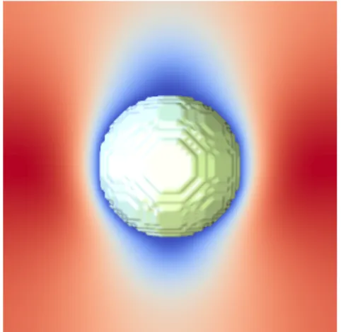
Figure 1: Example of velocity flow around a sphere.

Figure 1 shows an example plotted using Paraview of the velocity field around a spherical particle immersed in an horizontal flow.

5.2 Tomography picture

In this example we use a tomography picture of wood vessels (figure 2) from [6]. To avoid singularities at the boundary we added 15 voxels at the inlet and outlet using lzInf 15and lzSup 15commands in the simulation file.

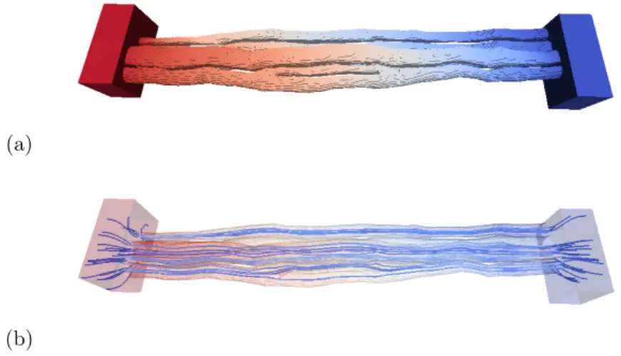
Figure 2: Tomography of wood vessels [6]. Note the two reservoir used to homogenize the pressure at the inlet and outlet of the domain.

Figure 3a and 3b show the pressure gradient and displays several stream lines in the sample.

(a)

(b)

Figure 3: Flow through wood vessels: (a) Pressure gradient; (b) Stream lines

Figures 5.2a and 5.2b display velocity profiles in several cross sections perpendicular to the flow direction.

(a) (b)

Figure 4: (a) magnitude of velocity field (in color map) at di↵erent posi-tion in the sample. (b) Velocity in a slice plotted using glyph vectors.

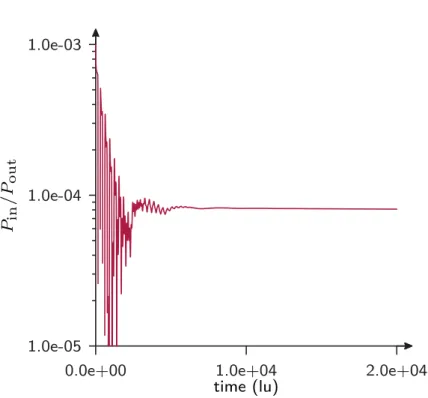
In figure 5 we plotted in semi-log axis the ratio of Pin and Pout as a function of time (in lattice units). After a rapid fluctuating domain the flow becomes stationary.

RXy2@y8

RXy2@y9

RXy2@yj

yXy2Yyy

RXy2Yy9

kXy2Yy9

P

fP

iBK2 UHmV

Figure 5: Evolution of Pin/Pout as a function of time.

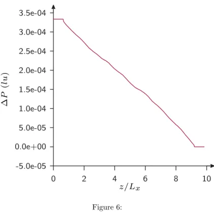
In the stationary regime, we plot in figure 6 the average pressure evolution in z slices as a function of z/Lx. Where Lx is the size of the sample in x direction. This evolution is a straight line grow which it is possible to determine the permeability using the Darcy law.

@8Xy2@y8

yXy2Yyy

8Xy2@y8

RXy2@y9

RX82@y9

kXy2@y9

kX82@y9

jXy2@y9

jX82@y9

y

k

9

e

3

Ry

ë

P

Ulu

V

z

fL

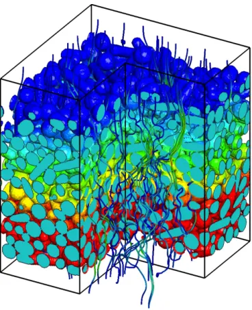
In this section we give an example in which the samples has been compute form Monte Carlo simulations. This sample is composed of particles of di↵erent sizes packed together in a periodic cell. Figure 7a shows a magnified picture of the particles and figure 7b the sample rasterized sample used in FLOWbox .

(a) (b)

Figure 7: (a) Packing of particles; (b) Rasterized sample.

The figure 8 shows the pressure gradient and streamlines through the packing plotted using Tecplot.

Figure 8: Flow through a sample of spherocylindrical particles of di↵erent length.

References

[1] P.L. Bathnagar, E.P. Gross, and M. Krook. A model for collision processes in gases, I. small amplitude processes in charged and neu-tral one-component system. Physical Review E, 94:511–25, 1954. [2] M. Bouzidi, M. Firdaouss, and P. Lallemand. Momentum

trans-fer of a boltzmann-lattice fluid with boundaries. Physics of Fluids, 13:3452–3459, 2001.

[3] S. Chapman and T.G. Cowling. The mathematical theory of nonuni-form gases. Cambridge University Press, 1970.

[4] Y. T. Feng, K. Han, and D. R. J. Owen. Coupled lattice boltz-mann method and discrete element modelling of particle transport in turbulent fluid flows: Computational issues. International Journal For Numerical Methods In Engineering, 72(9):1111–1134, November 2007.

[5] Z. G. Feng and E. E. Michaelides. The immersed boundary-lattice boltzmann method for solving fluid-particles interaction problems. Journal of Computational Physics, 195(2):602–628, April 2004. [6] X. Frank, G. Almeida, and P. Perr´e. Multiphase flow in the

vas-cular system of wood: From microscopic exploration to 3-d lattice boltzmann experiments. International Journal of Multiphase Flow, 36:599–607, 2010.

[7] X. He and L.-S. Luo. A priori derivation of the lattice boltzmann equation. Physical Review E, 55:R6333–R6336, 1997.

[8] K. Iglberger, N. Th¨urey, and U. R¨ude. Simulation of moving particles in 3d with the lattice boltzmann method. Computers & Mathemat-ics, 55:1461–1468, 2008.

[9] P. Lallemand and L. S. Luo. Lattice boltzmann method for moving boundaries. Journal of Computational Physics, 184(2):PII S0021– 9991(02)00022–0, 2003.

[10] A. Satoh. Introduction to the practice of molecular simulation. El-sevier Insights, 2011.

[11] D. Z. Yu, R. W. Mei, L. S. Luo, and W. Shyy. Viscous flow compu-tations with the method of lattice boltzmann equation. Progress In Aerospace Sciences, 39(5):329–367, July 2003.

[12] Zhaosheng Yu and Anthony Wachs. A fictitious domain method for dynamic simulation of particle sedimentation in bingham fluids. Journal of Non-Newtonian Fluid Mechanics, 145(2–3):78–91, 9 2007.