Algorithms for Routing Problems in Stochastic
Time-Dependent Networks
by
Seong-Cheol Kang
Submitted to the Department of Civil and Environmental Engineering
and the Operations Research Center
in partial fulfillment of the requirements for the degrees of
Master of Science in Transportation
and
Master of Science in Operations Research
at the
MASSACHUSETTS INSTITUTE OF TECHNOLOGY
February 2002
@
Massachusetts Institute of Technology 2002. All rights reserved.
MASSAC HUSETT1 N§TITUTE OF TECHNOLOGY
MAR 0
6
2002
LIBRARIES
8AhX
A uthor ...
Department A Civil and Environmental Engxeering
and Operations Research Center
September 29, 2001
Certified by...
Ismail Chabini
Assistat Professor of Civil and Environmental Engineering
Thesis Supervisor
Accepted by ...
...
James B. Orlin
Edwara Pennell Brooks Professor of Operations Research
Codirector, Operations Research Center
Accepted by ...
Oral Buyukozturk
Chairman, Departmental Committee on Graduate Studies
Algorithms for Routing Problems in Stochastic Time-Dependent
Networks
by
Seong-Cheol Kang
Submitted to the Department of Civil and Environmental Engineering and the Operations Research Center
on September 29, 2001, in partial fulfillment of the requirements for the degrees of
Master of Science in Transportation and
Master of Science in Operations Research
Abstract
This thesis considers routing problems in stochastic time-dependent networks where link travel times are modeled as time-dependent discrete random variables. Among various routing problems that arise in stochastic time-dependent networks, we focus on the follow-ing three problem classes: the minimum possible travel time path problem, the minimum expected travel time next-arc hyperpath problem, and the minimum expected travel time path problem.
In the first problem class, we study the all-to-one minimum possible travel time paths problem, the all-to-one minimum possible travel cost paths problem, the all-to-one k-mini-mum path travel time realizations problem, and the all-to-one k-dynamic shortest paths problem. As routing problems in the second problem class, we discuss the all-to-one mini-mum expected travel time next-arc hyperpaths problem, the all-to-one minimini-mum expected travel cost arc hyperpaths problem, the all-to-one minimum expected travel time next-arc hyperpaths problem in signalized networks, and the all-to-one minimum expected travel time next-arc hyperpaths problem in multimodal networks. Finally, we explore the all-to-one minimum expected travel time paths problem that belongs to the third problem class.
We drive optimality conditions for each routing problem. We develop efficient solution algorithms for the routing problems in the first two problem classes. We prove that the algorithms developed in the thesis have theoretically better worst-case running time com-plexities than the existing algorithms in the literature. Computational tests show that our algorithms outperform the existing algorithms in practice as well.
Thesis Supervisor: Ismail Chabini
Acknowledgments
First and foremost, I would like to thank my family-my parents, brother, sisters, nephews, and nieces for their love, blessing, and support. Had it not been for their constant encour-agement, this work could not have been done. I love them all and dedicate this thesis to them.
I wish to thank Professor Ismail Chabini for being my research advisor. I also would like to thank Professor Cynthia Barnhart, Professor Moshe Ben-Akiva, and Professor Nigel Wilson for their constructive advice.
I am deeply grateful to Professor Robert Freund and Professor Dimitris Bertsimas for their unconditional support. Their encouragement, guidance, and help can never be repaid fully.
Special thanks go to Professor Ikki Kim at Hanyang University in Korea. His heartfelt counsel cheered me up when I was frustrated.
Finally, I would like to thank my friends at the Center for Transportation Studies, at the Operations Research Center, and elsewhere at MIT for their help and friendship.
Contents
1 Introduction 19 1.1 Research Background . . . .. . . . .. . 19 1.2 Network Types . . . . 21 1.3 Problem Variants . . . . . . .. . . 23 1.4 Contributions . . . . 241.5 Outline of the Thesis . . . . 24
2 Literature Review 27 2.1 Routing Problems in Stochastic Static Networks . . . . 27
2.2 Routing Problems in Deterministic Time-Dependent Networks . . . . 29
2.3 Routing Problems in Stochastic Time-Dependent Networks . . . . 30
3 Preliminaries 33 3.1 Notation, Terminologies, and Assumptions . . . . 33
3.1.1 N etw ork . . . . 33
3.1.2 Time Period of Interest . . . . 34
3.1.3 Link Travel Times . . . . 34
3.1.4 Path Travel Times . . . . 35
3.1.5 Other Notation and Assumptions . . . . 38
3.2 Time-Space Network . . . . 39
3.2.1 Time-Space Network of a Deterministic Time-Dependent Network . 39 3.2.2 Time-Space Network of a Stochastic Time-Dependent Network . . . 42
4 Minimum Possible Travel Time Paths 49
4.1 Introduction ... ... 49
4.1.1 An Illustrative Example ... 50
4.1.2 Reasons to Study the Problem . . . . 51
4.2 Optimality Conditions . . . . 52
4.3 Minimum Possible Travel Time Paths in the Static Domain . . . . 57
4.4 Paths Construction . . . . 58
4.5 Solution Algorithms . . . . 59
4.5.1 Algorithm MPTTP . . . . 60
4.5.2 Algorithm LEAST . . . . 63
4.5.3 Comparison of the Algorithms . . . . 66
4.6 Exact Probability of the Minimum Possible Travel Time . . . . 66
4.7 Extensions . . . . 71
4.7.1 All-to-One Minimum Possible Travel Cost Paths Problem . . . . 73
4.7.2 All-to-One k-Minimum Path Travel Time Realizations Problem . . 79
4.7.3 All-to-One k-Dynamic Shortest Paths Problem . . . . 84
4.8 W aiting at Nodes . . . . 85
4.8.1 All-to-One Minimum Possible Travel Time Paths Problem . . . . 87
4.8.2 All-to-One Minimum Possible Travel Cost Paths Problem . . . . 88
4.8.3 All-to-One k-Minimum Path Travel Time Realizations Problem . . 88
4.8.4 All-to-One k-Dynamic Shortest Paths Problem . . . . 89
5 Minimum Expected Travel Time Next-Arc Hyperpaths 91 5.1 Routing Policies and Expected Travel Time-based Routing Problems . . . . 91
5.1.1 An Illustrative Example and Observations . . . . 92
5.1.2 Problem Type to Study . . . . 95
5.2 The Wait-and-See Expected Minimum Travel Time . . . . 95
5.3 Optimality Conditions . . . . 99
5.4 Minimum Expected Travel Time Next-Arc Hyperpaths in the Static Domain 101 5.5 Hyperpaths Construction . . . . 102
5.6 Solution Algorithms . . . . 102
5.7 5.8
5.6.2 Algorithm ELB . . . . Waiting at Nodes ...
Extensions . . . .
5.8.1 Minimum Expected Travel Cost Next-Arc Hyperpaths 5.8.2 Signalized Networks . . . . 5.8.3 Multimodal Networks . . . . 105 105 107 107 111 118
6 Minimum Expected Travel Time Paths 125
6.1 Optimality Conditions . . . . 126
6.2 Inherent Difficulty of the Problem . . . . 129
6.3 Solution Algorithms . . . . . . .. 131 6.3.1 Algorithm METTH-based-METTP . . . . 131 6.3.2 Algorithm METTP-B&B . . . . 133 6.3.3 Algorithm EV . . . . 135 6.3.4 Algorithm METTP . . . . 136 7 Computational Tests
7.1 Generation of Stochastic Time-Dependent Networks . . . . 7.2 Computational Test Results . . . .
7.2.1 All-to-One Minimum Possible Travel Time Paths Problem . . . .
7.2.2 All-to-One k-Minimum Path Travel Time Realizations Problem . .
7.2.3 All-to-One k-Dynamic Shortest Paths Problem . . . . 7.2.4 All-to-One Minimum Expected Travel Time Next-Arc Hyperpaths P roblem . . . .
7.3 Concluding Remarks . . . .. . . . .. .
8 Conclusions and Future Research Directions
8.1 C onclusions . . . .
8.1.1 Minimum Possible Travel Time Path Problem . . . .
8.1.2 Minimum Expected Travel Time Next-Arc Hyperpath Problem . . .
8.1.3 Minimum Expected Travel Time Path Problem . . . . 8.1.4 Results of Computational Tests . . . .
8.2 Future Research Directions . . . .
139 139 141 141 142 143 148 149 153 153 153 154 154 155 155
A Notation 157
A.1 Network-related Notation . . . . 157
A.2 Random Variable-related Notation . . . 158
A.3 Decision Variable-related Notation . . . 161
A.4 Miscellaneous Notation . . . . 162
B Example of Minimum Possible Travel Time Paths Computation 165
C Example of Minimum Expected Travel Time Next-Arc Hyperpaths
Com-putation 177
List of Figures
1-1 An Example of Deterministic Static Network . . . . 1-2 An Example of Stochastic Static Network . . . .
1-3 An Example of Deterministic Time-Dependent Network . . . . 1-4 An Example of Stochastic Time-Dependent Network . . . .
3-1 An Example Network . . . . 3-2 An Example of Deterministic Time-Dependent Network . . . .
3-3 Time-Space Network of the Deterministic Time-Dependent Network in Fig-ure 3-2, H = 6
3-4
3-5
3-6
An Example of 3-Dimensional Time-Space Network . . . . An Example of Stochastic Time-Dependent Network . . . . Time-Space Network of the Stochastic Time-Dependent Network in Figure 3-5, H = 6 . . . .
3-7 A Next-Arc Hyperpath Example . . . .
4-1 4-2 4-3 4-4 5-1 5-2 5-3 5-4 5-5 5-6 An Example Network . . . . An Example Network . . . . An Example Network . . . .
Time-Space Network of the Network in Figure 4-3, H = 6 An Example Network . . . .
Minimum Expected Travel Time Path . . . . Minimum Expected Travel Time Next-Arc Hyperpath . . An Example Network . . . .
Minimum Expected Travel Time Next-Arc Hyperpath . . Movements at a Signalized Intersection . . . .
21 21 22 22 36 39 . . . . 4 1 42 44 45 46 . . . . . 50 . . . . . 67 . . . . . 69 . . . . . 72 . . . . . 92 . . . . . 93 . . . . . 94 . . . . . 96 . . . . . 98 . . . . . 112
6-1 An Example Network . . . . 130 6-2 An Example Network . . . . 138
B-1 An Example Network ... ... 165
C-1 Minimum Expected Travel Time Next-Arc Hyperpath from Node 1 to Node
4 at Departure Time 0 ... ... 184
C-2 Minimum Expected Travel Time Next-Arc Hyperpath from Node 1 to Node
4 at Departure Time 1 . . . . 184
C-3 Minimum Expected Travel Time Next-Arc Hyperpath from Node 1 to Node
List of Tables
3.1 Time-Dependent Link Travel Time PMFs . . . . 36
4.1 Time-Dependent Link Travel Time PMFs ... 50
4.2 Path Travel Time Realizations . . . . 51
4.3 Minimum Possible Travel Times, Their Probabilities, and Selected Paths . 51 4.4 Time-Dependent Link Travel Time PMFs . . . . 67
4.5 Path Travel Time Realizations . . . . 68
4.6 Time-Dependent Link Travel Time PMFs . . . . 69
4.7 Path Travel Time Realizations from Node 1 to Node 5 at Departure Time 0 70 5.1 Time-Dependent Link Travel Time PMFs . . . . 93
5.2 Routing Strategies . . . . 94
5.3 Time-Dependent Link Travel Time PMFs . . . . 96
5.4 Network States and Minimum Travel Times . . . . 97
5.5 Signal Phases . . . . 113
5.6 Penalties (units of time) . . . . 113
7.1 Running Times of Algorithm LEAST and Algorithm MPTTP2 as a Function of H and R When n = 1000 and m = 4000 . . . . 142
7.2 Running Times of Algorithm LEAST and Algorithm MPTTP2 as a Function of H and R When n = 2000 and m = 8000 . . . . 142
7.3 Running Times of Algorithm LEAST and Algorithm MPTTP2 as a Function of H and R When n = 3000 and m = 12000 . . . . 143
7.4 Running Times of Algorithm k-LEAST and Algorithm k-MPTTR as a Function of H and R When n=200, m=800, and k = 5 . . . . 144
7.5 Running Function 7.6 Running Function 7.7 Running Function 7.8 Running Function 7.9 Running Times of of H and Times of of H and Times of of H and Times of of H and Times of Function of H and
Algorithm k-LEAST and Algorithm k-MPTTR as a
R When n = 200, m = 800, and k = 10 ...
Algorithm k-LEAST and Algorithm k-MPTTR as a
R When n = 600, m = 2400, and k = 5 ...
Algorithm k-LEAST and Algorithm k-MPTTR as a R When n = 600, m = 2400, and k = 10 ...
Algorithm k-LEAST and Algorithm k-MPTTR as a R When n = 1000, m = 4000, and k = 5 ...
Algorithm k-LEAST and Algorithm k-MPTTR as a R When n = 1000, m = 4000, and k = 10 ...
7.10 Running Times of Algorithm k-D-LEAST and Algorithm k-DSP as a
Func-tion of H When n = 1000, m = 4000, and k = 5 . . . . 146 7.11 Running Times of Algorithm k-D-LEAST and Algorithm k-DSP as a
Func-tion of H When n = 1000, m = 4000, and k = 10 . . . . 146
7.12 Running Times of Algorithm k-D-LEAST and Algorithm k-DSP as a Func-tion of H When n = 2000, m = 8000, and k = 5 . . . . 146 7.13 Running Times of Algorithm k-D-LEAST and Algorithm k-DSP as a
Func-tion of H When n = 2000, m = 8000, and k = 10 . . . . 147
7.14 Running Times of Algorithm k-D-LEAST and Algorithm k-DSP as a Func-tion of H When n = 3000, m = 12000, and k = 5 . . . . 147
7.15 Running Times of Algorithm k-D-LEAST and Algorithm k-DSP as a
Func-tion of H When n = 3000, m = 12000, and k = 10 . . . . 147
7.16 Running Times of Algorithm ELB and Algorithm METTH as a Function of H and R When n = 1000 and m = 4000 . . . . 149 7.17 Running Times of Algorithm ELB and Algorithm METTH as a Function of
H and R When n = 2000 and m = 8000 . . . . 149 7.18 Running Times of Algorithm ELB and Algorithm METTH as a Function of
H and R When n = 3000 and m = 12000 . . . . 150
7.19 Variances of Running Times of Algorithm LEAST and Algorithm MPTTP2
When n = 3000, m = 12000, H = 60, and R = 5 . . . . 150 7.20 Variances of Running Times of Algorithm k-LEAST and Algorithm k-MPTTR
When n = 1000, m = 4000, H = 60, R = 5, and k = 10 . . . . 151 144 144 145 145 145
7.21 Variances of Running Times of Algorithm k-D-LEAST and Algorithm k-DSP
When n = 3000, m = 12000, H = 60, and k = 10 7.22 Variances of Running Times of Algorithm ELB
When n = 3000, m = 12000, H = 60, and R = 5
Time-Dependent Link Travel Time PMFs . . . .
Time-Dependent Link Travel Time PMFs (cont.) Time-Dependent Link Travel Time PMFs (cont.) Time-Dependent Link Travel Time PMFs (cont.) Time-Dependent Link Travel Time PMFs (cont.) Time-Dependent Link Travel Time PMFs (cont.) R esults . . . .
151 and Algorithm METTH
. . . . 151 . . . . 165 . . . . 166 . . . . 166 . . . . 166 . . . . 166 . . . . 166 . . . . 175 C.1 Results . . . . 183 B.1 B.2 B.3 B.4 B.5 B.6 B.7
List of Algorithms
Algorithm MPTTP ... Algorithm MPTTP2 ... Algorithm LEAST ... Algorithm MPTCP ... Algorithm k-MPTTR ... Algorithm k-DSP ... Algorithm Hyperpath ... Algorithm METTH ... Algorithm ELB ... Algorithm METCH ... Algorithm METTH-Signal... Algorithm METTH-Multimodal Algorithm METTH-based-METTP Algorithm METTP-B&B ... Algorithm METTP ... 1 2 3 4 5 6 7 8 9 10 11 12 13 14 15 .. . 61 .. . 64 . . . 65 . . . 78 . . . 83 .. . 86 103 104 106 110 117 124 132 134 137Chapter 1
Introduction
1.1
Research Background
Routing people, vehicles, goods, messages, or other commodities over transportation or communication networks has been an important issue in satisfying economical and societal needs. When commodities are sent over a network, there usually exist one or more criteria
by which routes for the commodities are determined. For instance, individuals on their
way to work in the morning may want to take routes with the shortest travel times. A telecommunication company may want to route calls over a communication network in such a way that it accommodates as many calls as possible and also maintains a delay for each call below a certain level. Among various criteria, travel time between an origin and a destination serves as the primary concern in many routing applications.
Traditionally, routing problems were considered over deterministic static networks where link travel times are deterministic and time-invariant, i.e. they are fixed quantities. Many routing problems in deterministic static networks, whose objectives were mainly to find shortest paths, were successfully investigated and many efficient solution algorithms were developed as a result.
Researchers and practitioners then began to consider dynamism associated with link travel times and to use deterministic time-dependent networks, where link travel times change time-dependently, as base networks for various routing problems. With the advent of the Intelligent Transportation Systems (ITS), deterministic time-dependent networks became more important especially in transportation area because time-dependent travel time information was required to successfully deploy several subsystems of ITS such as
the Advanced Traveler Information Systems (ATIS) and the Advanced Traffic Management
Systems (ATMS).
In deterministic time-dependent networks, it is assumed that the travel time on a link varies according to the entry time to the link. It is also assumed that for a given link entry time, the link travel time is a constant that is known a priori with certainty. Although deter-ministic time-dependent networks approximate well real transportation or communication networks where network characteristics change according to the time of day and therefore have been extensively used for various routing problems for the last decade, a couple of drawbacks of deterministic time-dependent networks especially for transportation networks have been pointed out.
Firstly, we know from daily experience that even for the same link entry time, traversing a link may take different amounts of time in congested transportation networks, because of traffic volume change, incidents, meteorological condition, or other factors. Secondly, we do not know the travel time on a link in advance until we complete traversing the link. Therefore one of the assumptions of deterministic time-dependent networks, which is the travel time on a link is an a priori known constant with certainty for a given link entry time, is not valid in congested transportation networks.
In order to obtain more realistic routing solutions by modeling actual transportation networks better, it is imperative to take into consideration the variability and uncertainty of a link travel time for a given link entry time. A natural approach to capture the variabil-ity and uncertainty of a link travel time would be to consider a link travel time for a given link entry time as a random variable. This approach results in stochastic time-dependent networks where link travel times are random variables that have different probability dis-tributions according to link entry times.
Consideration of both stochasticity and time-dependency of link travel times makes routing problems much harder to solve. Presumably this is one of the reasons that active research on routing problems in stochastic time-dependent networks has begun recently and only a small number of research papers have been published. However, since stochasticity and dynamism are becoming increasingly important issues that cannot be ignored in many routing applications in transportation or communication networks, we expect stochastic time-dependent networks to take the place of deterministic time-dependent networks as base networks for various routing problems in the very near future.
This thesis studies several routing problems in stochastic time-dependent networks from a transportation application perspective. Particularly we focus on the development of fast solution algorithms for the routing problems with the intention of utilizing the algorithms for real time ITS applications.
1.2
Network Types
We may think of four network types depending on which of stochasticity and time-depen-dency of link travel times is considered. We illustrate the network types with examples in this section.
A deterministic static network has fixed link travel times as exemplified in Figure 1-1.
No stochasticity and time-dependency of link travel times exist. If another attribute of a link other than travel time is used, the value of the link attribute can be negative.
2
3 2
S3 4
Figure 1-1: An Example of Deterministic Static Network
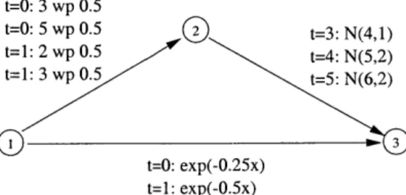
Figure 1-2 shows an example of stochastic static network. In networks of this type, the travel time on a link is a random variable. For instance, the travel time on link (2,3) follows a normal distribution with the mean of 4 and the variance of 1. Link travel time random variables may be discrete or continuous. There is no time-dependency of link travel times, so only one probability distribution is associated with each link. It is well known that we
3 wp 0.5
5 wp 0.5 N(4,1)
S3 exp(-0.25x)
can find a path with the minimum expected travel time from an origin to a destination
by setting each link travel time to its expected value and then applying a shortest path
algorithm (Sigal et al. [24], Eiger et al. [9]). Stochastic static networks have been widely used in the reliability analysis of communication or manufacturing networks and in the PERT-type network analysis for project management.
An example of deterministic time-dependent network is depicted in Figure 1-3. The travel time on a link has different values according to the link entry time. For instance, the travel time on link (1, 2) is 3 units of time when a traveler enters the link at time 0 and 5 units of time when he enters the link at time 1. As mentioned in the previous section, a link travel time is constant for a given link entry time. Link travel times and link entry times can be modeled in discrete time or in continuous time. Figure 1-3 shows a deterministic discrete time-dependent network.
2
t=0: 3 t=3: 4 t=1: 5 t=6: 3 3 t=0: 8 t=1: 7Figure 1-3: An Example of Deterministic Time-Dependent Network
Finally, Figure 1-4 illustrates an example of stochastic time-dependent network. For a given link entry time, the travel time on a link is obtained from a probability distribution that may be either discrete or continuous. For instance, the travel time on link (1, 3) is exponentially distributed, but the distribution has different parameters according to the
t=0: 3 wp 0.5 t=: 5 wp 0.5 2t=3:N(4,1) t=1: 2 wp 0.5 t=4: N(5,2) t=1: 3 wp 0.5 t=5: N(6,2) S3 t=0: exp(-0.25x) t=1: exp(-0.5x)
link entry time. Note that stochastic time-dependent networks can be thought the most general network type because they can reduce to networks of other types if one or both of stochasticity and time-dependency of link travel times is ignored. In this thesis, we consider stochastic time-dependent networks where probability distributions are discrete and link travel times as well as link entry times are also discrete.
1.3
Problem Variants
Unlike deterministic static or deterministic time-dependent networks, stochastic time-depen-dent networks may allow more than one path to have some positive probability of being shortest for any origin-destination pair. Therefore the shortest travel time is not a well-defined criterion for selecting routes in stochastic time-dependent networks.
We may employ other criteria by which routing decisions can be made unambiguously in stochastic time-dependent networks, such as the lowest possible travel time on a path, the longest possible travel time on a path, the expected travel time on a path, the variance of the travel time on a path, etc. In this thesis, we consider the following two criteria among others:
* Lowest Possible Travel Time * Expected Travel Time
In routing problems with the lowest possible travel time criterion, we want to find a path whose lowest possible travel time (minimum travel time) is smaller than that of any other path for an origin-destination pair at a given departure time. In the literature, routing problems of dispatching emergency vehicles in urban areas adopt this criterion (Miller-Hooks
[16], Miller-Hooks and Mahmassani [17]).
The expected travel time criterion is associated with another class of routing prob-lems where we want to find a path with the minimum expected travel time for an origin-destination pair at a given departure time.
It turns out that the expected travel time criterion results in a different class of routing problems if travelers are allowed to change their paths adaptively during their trips in stochastic time-dependent networks. This class of routing problems, called the minimum expected travel time next-arc hyperpath problem, is also studied in this thesis.
To recapitulate, the following three classes of routing problems are discussed in the thesis:
" Minimum Possible Travel Time Path Problem
" Minimum Expected Travel Time Path Problem
" Minimum Expected Travel Time Next-Arc Hyperpath Problem
Routing problems are further classified by the number of origins, the number of desti-nations, and the number of departure times. In the context of ITS applications, routing problems concerning all origins, a single destination, and all departure times (so-called all-to-one problems) are of particular interest. Therefore we will study various all-to-one routing problems in each problem class in this thesis.
1.4
Contributions
The contributions of the thesis are as follows:
" For each routing problem, we derive a set of optimality conditions that is a dynamic
programming formulation of the problem.
" For several routing problems in the first and the third problem classes (the minimum
possible travel time path problem and the minimum expected travel time next-arc hyperpath problem), we develop solution algorithms with worst-case optimal running time complexities.
" For other routing problems, we develop efficient solution algorithms that have better
worst-case running time complexities than the existing algorithms in the literature.
1.5
Outline of the Thesis
The thesis is organized in eight chapters. This first chapter mentions the research back-ground, the network types, the routing problem variants to be studied, and the contributions of the thesis. In Chapter 2, the related literature is reviewed. In Chapter 3, we present some preliminary material for the thesis, which includes basic notation, terminologies, assump-tions, the concept of time-space network, and the concept of next-arc hyperpath. We study
several routing problems that belong to the minimum possible travel time path problem class in Chapter 4. We discuss the characteristics of routing problems of this class. For each routing problem studied, we derive a set of optimality conditions and then develop an efficient solution algorithm from it. In Chapter 5, we first introduce two routing policies in stochastic time-dependent networks. We then distinguish between the minimum expected travel time next-arc hyperpath problem and the minimum expected travel time path prob-lem, based on routing policy. Several routing problems in the former problem class are studied in the chapter. For each routing problem, we derive a set of optimality conditions and develop an efficient solution algorithm. In Chapter 6, we discuss one problem in the minimum expected travel time path problem class, the all-to-one minimum expected travel time paths problem. We explain why this problem is inherently difficult to solve and dis-cuss ideas of possible solution algorithms. In Chapter 7, we report on the results of the computational tests on several algorithms presented in the preceding chapters. Finally, the conclusions and the future research directions are given in Chapter 8.
Chapter 2
Literature Review
In this chapter, we review the literature pertaining to routing problems in stochastic static networks, in deterministic time-dependent networks, and in stochastic time-dependent net-works. We do not survey the research work on routing problems in deterministic static networks because several textbooks summarizing the work, for instance Ahuja et al. [1] and Bertsekas [2], are readily available.
2.1
Routing Problems in Stochastic Static Networks
Most papers credit Frank [10] with the first published work on the "shortest" path problem in stochastic static networks. He considers the problem of computing the probability that the minimum travel time from an origin node to a destination node is less than some value when link travel times have continuous probability distributions. Notice that this problem is essentially equivalent to determining the probability distribution of the minimum travel time. To avoid the complications arising from the computation of multiple integrals, he approximates the computation by Monte Carlo simulation. He also studies the comparison of any two disjoint paths from an origin node to a destination node based on the probability that the travel time on each path is greater than a given threshold. He recognizes that the computation of this probability involves a convolution of link travel time random variables, which is formidable when each path contains many links. He overcomes this difficulty by using the central limit theorem. In addition, he discusses hypothesis tests on the probability that the minimum travel time from an origin node to destination node is greater than some specified value.
Sigal et al. [24] consider the selection of the "shortest" path from an origin node to a destination node when link travel time random variables are independent of each other. As a performance measure of a path to be used in determining the "shortest" path, they introduce the concept of a path optimality index. The optimality index of a path is defined as the probability that the path is shorter than all other paths. They recognize that the optimality index of a path is difficult to compute, because links may belong to more than one paths and therefore path travel times are not independent random variables. They resolve the statistical dependence among path travel times by using the concept of uniformly directed cutsets and present an analytical procedure to compute the optimality index of a path. The analytical procedure, however, involves multiple integrals that are difficult to evaluate in practice.
Eiger et al. [9] study the problem of finding an optimal path from an origin node to a destination node when a traveler uses a utility function to evaluate each path. The utility function is a nonincreasing function of the travel time on a path. An optimal path is defined as one with the maximum expected utility. They show that when link travel times are independent random variables and the utility function is linear or exponential, an efficient Dijkstra-type algorithm can solve the problem.
Mirchandani and Soroush [19] extend the work of Eiger et al. [9] to the problem with a quadratic utility function. In this case, Dijkstra-type algorithms may not find an optimal path. They propose an algorithm that depends on only the first and second moments of the travel time on a path, but it has an exponential running complexity in the worst case.
Kulkarni [14] considers networks where link travel times are independent and exponen-tially distributed random variables. From the network, he constructs a continuous time Markov chain (CTMC) with a single absorbing state such that the time until absorption into the absorbing state starting from the initial state is equal to the minimum travel time from a given origin node to a given destination node in the network. Using the Markov chain, he develops methods for computing the distribution of the minimum travel time, the moments of the minimum travel time, and the optimality index of a path. His approach has a limitation that the state space of the Markov chain may grow exponentially with the network size. Hence this approach is not suitable for large dense networks.
Extending the work of Kulkarni [14], Corea and Kulkarni [6] present methods for com-puting the distribution and moments of the minimum travel time in networks where link
travel times are independent, nonnegative, and integer valued random variables. They use a discrete time Markov chain (DTMC) with a finite state space and a single absorbing state. The same drawback as in Kulkarni [14] exists in this approach too.
2.2
Routing Problems in Deterministic Time-Dependent
Net-works
Perhaps the earliest paper dealing with routing problems (shortest path problems) in deter-ministic time-dependent networks can be attributed to Cooke and Halsey [5]. They present a recursive functional form (a set of optimality conditions) that gives the shortest paths from all nodes to one destination node for all discrete departure times.
Dreyfus [8] suggests a label-setting approach which generalizes Dijkstra's algorithm to determine the shortest path between two nodes for a given departure time.
Kaufman and Smith [13] show a counterexample for which Dreyfus' approach fails to detect the shortest path. They establish a consistency condition under which Dijkstra-type algorithms (Dreyfus' approach) are guaranteed to find the shortest path with the same computational complexity as that of the static shortest path problem. This consistency condition is thought of as the first-in first-out (FIFO) condition.
Ziliaskopoulos and Mahmassani [26] propose a label-correcting algorithm that deter-mines the shortest paths from all nodes to one destination node for all discrete departure times. The algorithm does not require the FIFO condition to hold in the network. It can handle the case where an attribute of a link other than travel time, which can have a negative value, is used, as long as the network does not have negative "cost" cycles.
Chabini [3] considers three routing problems: the shortest paths from one origin node to all other nodes for a given departure time (called the one-to-all shortest paths problem), the shortest paths from all nodes to one destination node for all discrete departure times (called the all-to-one shortest paths problem), and the minimum cost paths from all nodes to one destination node for all discrete departure times (called the all-to-one minimum cost paths problem). He reviews optimality conditions for each problem. He then develops decreasing order of departure time (DOT) algorithms for the all-to-one shortest paths problem and the all-to-one minimum cost paths problem. He shows that the two algorithms have the optimal running time complexities, and that consequently no algorithms with better running
time complexities can be found for the problems. The ideas underlying those decreasing order of departure time algorithms will be extended to routing problems in stochastic time-dependent networks in this thesis.
Chabini and Dean [4] present a deeper analysis of waiting at nodes. They develop a decreasing order of departure time algorithm for the all-to-one shortest paths problem and an increasing order of departure time (IOT) algorithm for the one-to-all shortest paths problem, when waiting at nodes is allowed in the network.
2.3
Routing Problems in Stochastic Time-Dependent
Net-works
Hall [12] appears to be a seminal paper about routing problems in stochastic time-dependent networks. He shows that static shortest path algorithms such as Dijkstra's algorithm may not find the minimum expected travel time path between two nodes for a given departure time in stochastic time-dependent networks. He proposes an algorithm that finds the min-imum expected travel time path from one origin node to one destination node for a given departure time. The algorithm combines a branch-and-bound technique and a k-shortest paths algorithm. Although the algorithm is exact, it does not explain how to compute the expected travel time on a given path. The algorithm will be reviewed in Chapter 6 of this thesis. He also realizes that the best route from any intermediate node to the destination in terms of expected travel time depends on the arrival time at that intermediate node. Therefore the best route can be found by deferring the choice of the next link to take until the intermediate node is reached. He calls this method the time-adaptive route choice. The result obtained from the time-adaptive route choice is generally not a simple path, but it is referred to as an optimal adaptive decision rule (it is called the minimum expected travel time next-arc hyperpath in this thesis). He applies dynamic programming to the problem of finding an optimal adaptive decision rule from one origin node to one destination node for a given departure time. We will study related problems in Chapter 5.
Kaufman and Smith [13] briefly mention a consistency condition for the determination of the minimum expected travel time path in stochastic time-dependent networks. However they do not propose any solution algorithm.
net-works where link travel times are independent discrete random variables. She proposes several efficient solution algorithms, some of which will be revisited in this thesis.
Miller-Hooks and Mahmassani [17] discuss the problem of finding a path with the min-imum possible travel time from all nodes to one destination node for all discrete departure times when link travel times are independent discrete random variables. They extend the problem to selecting several paths from all nodes to one destination node for all discrete departure times. These two problems will be studied in detail in Chapter 4.
Fu and Rilett [11] study the problem of finding the minimum expected travel time path from one origin node to one destination node for a given departure time when link travel times are modeled as continuous time stochastic processes, i.e. link travel times have continuous probability distributions. They claim that even if the link travel times are independent random variables, the probability distribution of the travel time on a path is very hard to obtain from the probability distributions of the travel times on the links constituting the path. Hence they study how to estimate the expected travel time on a path by using the means and variances of the travel times on the constituent links of the path. They present a heuristic algorithm for the problem, which relies on a k-shortest paths algorithm as well as the estimated expected travel time on a path.
Miller-Hooks and Mahmassani [18] propose an efficient algorithm for the problem of finding the minimum expected travel time next-arc hyperpaths from all nodes to one desti-nation node for all discrete departure times. They also present a non-polynomial algorithm for the problem of finding the minimum expected travel time paths from all nodes to one destination node for all discrete departure times. We will revisit these algorithms in Chap-ters 5 and 6.
Yang and Miller-Hooks [25] study the problem of finding the minimum expected travel time next-arc hyperpaths from all nodes to one destination node for all discrete departure times in signalized networks. This problem will be discussed in Chapter 5.
Opasanon and Miller-Hooks [21] consider stochastic time-dependent multimodal net-works. They study the problem of finding the minimum expected travel time next-arc hyperpaths from all nodes to one destination node for all discrete departure times in such networks. This problem will be also discussed in Chapter 5.
Chapter 3
Preliminaries
In this chapter, we present preliminary material for this thesis. In Section 3.1, we introduce basic notation, terminologies, and assumptions that will be used throughout the thesis. Other problem-specific notation, terminologies, and assumptions will be introduced where appropriate in the thesis. The comprehensive set of notation is summarized in Appendix A. We also introduce the concepts of time-space network and next-arc hyperpath in Section
3.2 and in Section 3.3, respectively.
3.1
Notation, Terminologies, and Assumptions
3.1.1 Network
Consider a network consisting of a finite number of nodes and a finite number of directed links. We denote such a network by
S
= (N, A), where N is the set of n nodes and A is the set of m directed links.Let d denote a given destination node. The network is assumed to have at least one directed path from every node to the destination node d. It is assumed that no parallel links exist between any two nodes, thus we have m < n(n - 1).
We denote by 0(i) the set of end nodes of outgoing links from node i, i.e. 0(i) =
{j
I
(i, j) E A}. Similarly, we denote by J(i) the set of start nodes of incoming links to node i,
3.1.2
Time Period of Interest
Let J* = [ti, t] be a continuous time period of interest, which is generally a peak period of the network. We discretize {* into small time intervals. Let YC = {ti, ti + At, t +
2At,... , ti
+
(H - 1)At} be a discretized time period of interest, where At is the length of each small time interval and tj + (H - 1)At = t,. At should be chosen such that it is no greater than any link travel time value. This allows us to avoid the case where one would arrive at a next node at the same time interval as the departure time from a node, which is not realistic from a practical point of view.For the sake of brevity of exposition hereafter, without loss of generality, we assume that t1 = 0 and At = 1. Thus the discretized time period of interest becomes the set
H = {0, ... , H - 1}.
3.1.3 Link Travel Times
We assume that link travel times are time-dependent random variables whose probability distributions vary according to the times that the links are entered.
For each link (i, j) E A and each link entry time t E H, let Tij (t) be a random variable denoting the travel time on link (i, j) when one enters the link at time t. We assume that the probability distribution of Tij(t) is discrete. The probability mass function (PMF) of
Ti (t) is denoted by pTj
(t)-We define a realization of Tij(t) as a couple of a possible travel time value and its probability. Let Tij(t) have rij(t) realizations denoted by (%rj(t),pr (t)), r E 'Ri(t) 3 =
{1, ... ,rij(t)}. 1r-r(t) is the travel time value of the rth realization of Tij(t). pr (t) is the probability of the rth realization of Ti3 (t) (the probability that Tri(t) occurs, i.e. P[Ti3 (t) = < (t)] = pr (t)). We assume that rr (t), V r E 'Rij (t) are distinct. We represent the PMF of Ti (t) by the set of realizations as follows:
PTj(t) = {(,ri(t), pi (t)) r E 'Ri (t) , (3.1)
where E tZej ti (t) = 1.
We assume that the link travel time values rr(t), V (i, j) E A, V t E H, V r E 'RZi (t) are
positive integers. We also assume that after the peak period, i.e. t > H - 1, the network
at a link entry time t > H - 1 is assumed to be the same as that of link (i, j) at the link
entry time t = H - 1. Mathematically, pT%,(t) =PTi(H-1), V(ij) E A, Vt > H - 1.
We denote by in the total number of link travel time realizations in the network during the peak period. Fn is given by
in-= 'Ii (t). (3.2)
(ij)EA tEX
As will be explained in Section 3.2.2, in- is the same as the number of links in the time-space network of a stochastic time-dependent network.
3.1.4 Path Travel Times
In stochastic time-dependent networks, the travel time on a path is also a time-dependent random variable because it is a function of the travel times of the links constituting the path, which are time-dependent random variables.
Let L'(t) be a random variable denoting the travel time on path c from node i to the destination node d at departure time t. Like a realization of a link travel time, we define a realization of Lj(t) as a couple of a possible travel time value and its probability. The realizations of L'(t) are not given data, but computed from the travel time realizations of the links on the path.
We denote the realizations of L'(t) by (l t ), (t)), k = 1,2, ... , ke(t), where ki(t) is the number of realizations. 1jk (t) is the travel time value of the kth realization of L'(t) and pi (t) is the probability that ly (t) occurs, i.e. P[Lc(t) = l t = p"(t). The PMF of L (t) is then represented by
PL (t) = {(lkt)jpik(t)) I k = 1,2, ... , k (t)}. (3.3) Let us illustrate how to construct the PMF of Lc(t) from the link travel time PMFs when the link travel times are independent random variables. Consider a trip from node 1 to node 3 at departure time 0 in the stochastic time-dependent network depicted in Figure
3-1 and Table 3.1. Let path a be 1 -+ 2 -+ 3 and path b be 1 - 3. Assuming that all
link travel time random variables are independent of each other, we obtain all travel time realizations of each path for this trip as follows:
Destination
Figure 3-1: An Example Network
Table 3.1: Time-Dependent Link Travel Time PMFs
Link (i, j) 1 (1, 2) (1, 3) (2,3) Departure Time (t) 0 0 1 2 (1, 0.5) (4, 0.5) (2, 0.4) (1, 0.8) ( ) ) (2, 0.5) (6, 0.5) (3, 0.6) (3, 0.2) * For path a: l (0) =Tr,2(0) + 7-3 22(+()) = 1 + 723(1) = 1
+ 2 = 3
P1 (0) = P12(0) x P23(0 + rT2(0)) -05 x P13(1) = 0.5 x 0.4 = 0.2 l12(0) =Tr,2(0) + r23(0 + 7-2(0)) = 1+ -r3 (1) = 1 + 3 = 4 ay2(0 = ()X p2s( +r1 7(0)) =0. 5 X p231 . . . p1 (0)= P12(0) 3(0 + 3(2) = 0.5 x 0.6=
0.3 a3 li (0) =Ti?2(0) +T 3(0 +? 2(0)) = 2+T 3(2) =2 +13 p12(0) = p 2(0) x P13(0 + r?2(0)) = 0.5 x P 13(2) = 0.5 x 0.8 = 0.4 1~()2(0)xp23(0 +T-12(0))0.5 Xp 2 (2) 05 x020.1 * For path b: 1 (0) =r,3(0) = 4 P (0) =Pi3(0) - 0.5 p16
l 2(0) = Tf3(0) = 6 1 (0)=p( 1i 3()0.5=0.5The PMFs of L'(0) and Li (0) are therefore given by
PL (o) =
{(3,
0.2), (4,0.3), (3, 0.4), (5, 0.1)}, (3.4)PLi(o) =
{(4, 0.5),(6,0.5)}.
(3.5)Note that the first and the third realizations of La(0) have the same travel time value, i.e. ja (0) = la' (0). The two path travel time realizations, however, are obtained by different
combinations of the link travel time realizations. The first realization is obtained by (Tr1 2 (0), P12(O)) and ('r 3(1),p$3(1)), whereas the third realization is obtained by (Tr2(O),p 2(0)) and
(-23(2), P23(2)). In the minimum possible travel time path problem that will be discussed
in Chapter 4, we will treat each travel time realization of a path obtained by a different combination of the link travel time realizations on the path differently, regardless of its travel time value. Hence the first and the third travel time realizations of path a in the above example are considered to be different realizations although they have the same travel time value. Consequently, we allow allow a PMF of path travel time to have more than one realization with the same travel time value as exemplified in (3.4).
Now we introduce several terminologies related to path travel time. For a given node
i, path c, and departure time t, mink{lk (t)} is referred to as the minimum travel time on path c from node i to node d at departure time t. A travel time realization of path c from node i to node d at departure time t, whose travel time value equals to the minimum travel time is called a minimum travel time realization. Since we differentiate between travel time realizations of a path, which have the same travel time value, but are obtained
by different combinations of the link travel time realizations on the path, there may exist
several minimum travel time realizations on path c from node i to node d at departure time t.
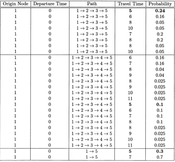
In the above example, the minimum travel time on path a from node 1 to node 3 at departure time 0 is 3 units of time. (3,0.2) and (3,0.4) are the minimum travel time realizations of path a at departure time 0. As for path b from node 1 to node 3, the mini-mum travel time at departure time 0 is 4 units of time and (4,0.5) is the minimini-mum travel time realization at departure time 0.
For a given node i and departure time t, we refer to minc{min{ly (t)}} as the minimum possible travel time from node i to node d at departure time t. We call a path travel time
realization from node i to node d at departure time t, whose travel time value equals to the minimum possible travel time a minimum possible travel time realization. More than one minimum possible travel time realization may exist from node i to node d at departure time t. Some of those realizations may belong to the same path.
The minimum possible travel time from node 1 to node 3 at departure time 0 in the above example is 3 units of time. (3,0.2) and (3,0.4) are the minimum possible travel time realizations from node 1 to node 3 at departure time 0. Both of the minimum possible travel time realizations belong to path a.
Note that the minimum travel time and a minimum travel time realization are the termi-nologies associated with each (origin node, path, departure time) triplet, while the minimum possible travel time and a minimum possible travel time realization are the terminologies
associated with each (origin node, departure time) pair.
3.1.5 Other Notation and Assumptions
Stochastic time-dependent networks are said to have the FIFO property if the following
conditions hold [17].
P[s + Tij(s) <; t + Ti(t)] = 1, V(ij) E A, Vt E X, Vs < t, 8 E H. (3.6)
If the networks have the FIFO property, solution algorithms for some routing problems could
be developed fairly easily. For instance, Dijkstra-type algorithms can solve the minimum possible travel time path problem. However it is a property that is not always satisfied in real transportation networks. In this thesis, we do not impose the FIFO property on the networks.
Concerning waiting at nodes, we assume that no waiting is allowed at all nodes in most part of the thesis. However we will provide short discussions about the case where waiting is allowed at all nodes in Chapters 4 and 5.
While developing solution algorithms for various routing problems in stochastic time-dependent networks in the subsequent chapters, we often need to solve an all-to-one shortest paths problem in deterministic static networks as an initialization step of the algorithms (details will be given in relevant parts of the thesis). We denote by 9(f(n, m)) the lowest possible running time to solve an all-to-one static shortest paths problem with n nodes and
m links.
3.2
Time-Space Network
3.2.1 Time-Space Network of a Deterministic Time-Dependent Network
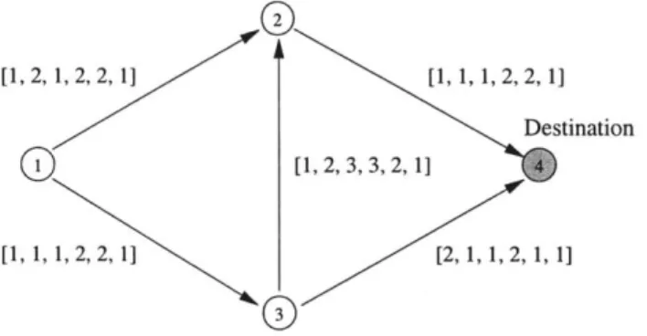
When a deterministic time-dependent network is graphically represented without explicitly incorporating time as a dimension, a vector of numbers which indicates time-dependent travel times is associated with each link as exemplified in Figure 3-2. In this figure, for instance, [1, 2,1, 2, 2] on link (1, 2) means that the traversal time of link (1, 2) is 1 unit of time at departure time 0, 2 at departure time 1, and so on.
2
[1, 2, 1, 2, 2, 11 [1, 1, 1, 2, 2, 1]
Destination [1, 2, 3, 3, 2,1]
[1, 1, 1, 2, 2, 1] [2, 1, 1, 2, 1, 1]
Figure 3-2: An Example of Deterministic Time-Dependent Network
This network representation, however, is not convenient for visualization of the net-work and algorithm development. Especially for the later purpose, we use the concept of
time-space network. A time-space network is a deterministic static network constructed
by expanding the original network in the time dimension. The following shows how to
construct the time-space network of a deterministic time-dependent network.
For each node i of the original network, we expand node i by creating node-time pairs
(i, t) for all t E X. We also create an additional node-time pair (i, H) which plays a role of all node-time pairs (i, t), V t > H - 1. Node-time pairs (i, t) E N x X U {H} are the set
of nodes of the time-space network. We introduce a link between two node-time pairs (i, t) and (j, s), if (i, j) E A and the travel time on link (i, j) at time t is s - t.
Let us denote the set of nodes and the set of links of the time-space network by
4
andN=
{(it)I
i E2,
t E a-u {H}},A
{((i, t), (j,
s))I
(i, j)
E A,t + rij(t) =
s,t
E C,where rij(t) is the deterministic travel time on link (i, j) of the
entry time t.
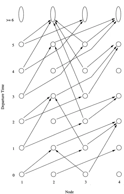
Figure 3-3 shows the time-space network of the deterministic depicted in Figure 3-2. Here are several observations about the deterministic time-dependent network.
(3.7) (3.8) E H U {H}} ,
original network at link
time-dependent network time-space network of a
1. The time-space network is a deterministic static network. Therefore any deterministic
static shortest path algorithm can be directly applied to the time-space network.
2. There exist a one-to-one correspondence between all paths in the time-space network and all paths in the original network.
3. If all link travel times of the original network are positive, then the corresponding
time-space network is acyclic.
4. By construction, no parallel links exist between any two nodes in the time-space network.
5. If waiting is allowed at node i of the original network from time t to time s (s > t),
then there exist links ((i, t), (i, t + 1)), ((i, t + 1), (i, t + 2)), ... , ((i, s - 1), (i, s)) in
the corresponding time-space network.1
6. The number of nodes in the time-space network is INI x IX U {H}I = n(H + 1).
7. The number of links in the time-space network is JAl x IHI = mH. If waiting is allowed at nodes, it is bound from above by (JAI +
lNI)
x19C
= (m + n)H.28. Let (((i, t)) be the set of end nodes of outgoing links from node (i, t) in the time-space
network. If ((i, t)) = {(j, si), (j2, S2),.- ,(jp, Sp)}, then ji 5 j2
#
-#Jp'This is valid only if the cost of waiting is additive (Chabini and Dean [4]). 2
This is valid only if the length of waiting is unlimited and the cost of waiting is additive (Chabini and Dean [4]).
>= 60 4 0 0 0 0 3 0 0 O 4o 2O 0 0 1 0 1 2 3 4 Node
Figure 3-3: Time-Space Network of the Deterministic Time-Dependent Network in Figure
We can also draw a time-space network using a three-dimensional diagram where one dimension represents departure time and the other two dimensions describe the spatial layout of the nodes in the original network (see Figure 3-4).
>= 6
0
0.2
..
0
DestinationFigure 3-4: An Example of 3-Dimensional Time-Space Network
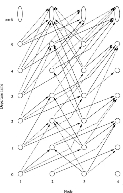
3.2.2 Time-Space Network of a Stochastic Time-Dependent Network Similar to deterministic time-dependent networks, we can construct the time-space network of a stochastic time-dependent network. In this case, the set of nodes of the time-space network is the same as X, but the time-space network has much more links because the travel time on link (i, j) of the original network may have several realizations for a given departure time.
Let
N
and A be the set of nodes and the set of links of the time-space network of a stochastic time-dependent network, respectively. ThenA= {((it),(js))
I
(ij) E A, t+T rj(t) = s, r E 'Rij(t), t E H, s E X U{H}} . (3.10)Several observations about the time-space network of a stochastic time-dependent net-work are as follows:
1. The time-space network is a deterministic static network. Therefore any deterministic
static shortest path algorithm can be directly applied to the time-space network. 2. Since we assume that all rjj (t) are positive, the time-space network is acyclic.
3. By construction, no parallel links exist between any two nodes in the time-space
network.
4. If waiting is allowed at node i of the original network from time t to time s (s > t), then there exist links ((i, t), (i, t + 1)), ((i, t + 1), (i, t + 2)), . . . , ((i, s - 1), (i, s)) in
the corresponding time-space network.3
5. The number of nodes in the time-space network is
1N
xPX
U {H}l = n(H + 1).6. The number of links in the time-space network is i = E(i'j)eA ZtEj-c ij M(t)I. If
waiting is allowed at nodes, it is bound from above by i
+
nH.47. Let 0((i, t)) be the set of end nodes of outgoing links from node (i, t) in the time-space network. If 6((i, t)) = {(ji, si), (j2, S2), ... , (jp, sp)}, then some of ji, j2, ,jp can
be identical.
Suppose there exist several paths between two nodes in the time-space network of a stochastic time-dependent network. From the last observation above, we can deduce that some of the topological paths corresponding to those paths could be identical. Note that all topological paths corresponding to paths between two nodes in the time-space network of a deterministic time-dependent network are distinct if waiting at nodes is not allowed in the deterministic time-dependent network.
The acyclic property of the time-space network of a stochastic time-dependent network will play a key role when we develop efficient algorithms for routing problems in stochastic time-dependent networks later in this thesis.
3
This is valid only if the cost of waiting is additive (Chabini and Dean [4]).
4
This is valid only if the length of waiting is unlimited and the cost of waiting is additive (Chabini and Dean [4]).
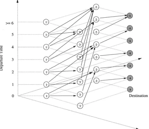
![Figure 3-5 shows an example of stochastic time-dependent network. For instance, [1, 2, 1, 2, 2, 1] wp 0.5 and [2, 1, 3, 3, 3, 2] wp 0.5 on link (1, 2) mean that P[T 12 (0) = 1] = 0.5, P[T 1 2 (0) = 2] = 0.5; P[T 1 2 (1](https://thumb-eu.123doks.com/thumbv2/123doknet/13925483.450141/44.918.290.680.293.474/figure-shows-example-stochastic-time-dependent-network-instance.webp)