Wind Mill Pattern Optimization using Evolutionary Algorithms

HAL Id: hal-02917483

https://hal-enac.archives-ouvertes.fr/hal-02917483

Preprint submitted on 19 Aug 2020

HAL is a multi-disciplinary open access

archive for the deposit and dissemination of

sci-entific research documents, whether they are

pub-lished or not. The documents may come from

teaching and research institutions in France or

abroad, or from public or private research centers.

L’archive ouverte pluridisciplinaire HAL, est

destinée au dépôt et à la diffusion de documents

scientifiques de niveau recherche, publiés ou non,

émanant des établissements d’enseignement et de

recherche français ou étrangers, des laboratoires

publics ou privés.

Wind Mill Pattern Optimization using Evolutionary

Algorithms

Charlie Vanaret, Nicolas Durand, Jean-Marc Alliot

To cite this version:

Charlie Vanaret, Nicolas Durand, Jean-Marc Alliot. Wind Mill Pattern Optimization using

Evolu-tionary Algorithms. 2020. �hal-02917483�

Wind Mill Pattern Optimization

using Evolutionary Algorithms

Charlie Vanaret

ENAC∗ , IRIT† 7 av Ed Belin 31055 Toulouse Cedex 5, France

vanaret@recherche.enac.fr

Nicolas Durand

ENAC, IRIT 7 av Ed Belin 31055 Toulouse Cedex 5, France

durand@recherche.enac.fr

Jean-Marc Alliot

IRIT 118 route de Narbonne 31062 Toulouse Cedex 9, France

jean-marc.alliot@irit.fr

ABSTRACT

When designing a wind farm layout, we can reduce the num-ber of variables by optimizing a pattern instead of consider-ing the position of each turbine. In this paper we show that when reducing the problem to only two variables defining a grid, we can gain up to 3% of energy output on simple exam-ples of wind farms dealing with many turbines (up to 1000) while dramatically reducing computation time. To achieve these results, we compared both a genetic algorithm and a differential evolution algorithm to previous results from the literature. These preliminary results should be extended to examples involving non-rectangular farm layouts and wind distributions that may require pattern deformation variables in order to increase solution diversity.

Categories and Subject Descriptors

J.6 [Computer-Aided Engineering]: Computer-aided de-sign; D.2.2 [Software Engineering]: Design Tools and Techniques—Computer-aided software engineering

Keywords

wind energy, wind farm layout, optimization

1.

INTRODUCTION

In the last 15 years, there has been growing interest and investment in renewable energy. Wind power capacity, for example, has risen from 17GW in 2000 to around 250GW in 2013, and the annual growth rate is currently between 10 and 20%. Consequently, the economic stakes and attempts to discover techniques for efficiently installing wind farms both onshore and offshore have increased dramatically; Gon-zalez’s recent review [2] lists almost 150 bibliographic refer-ences for the optimal wind-turbine micro-sitings problem. ∗

Ecole Nationale de l’Aviation Civile †

Institut de Recherche en Informatique de Toulouse

Because turbines create a wake vortex that reduces the wind flow for neighbouring units, packing as many wind turbines as possible in a given area is inefficient. There are different wake vortex models; in this paper, we use the park model de-scribed in [7] to compute these wake effects. In this model the wake effects created by all turbines j for j 6= i on a turbine i changes the wind resource available to i along dif-ferent directions by reducing the scale parameter c of the Weibull distribution estimated for the entire farm, which is also called the freestream wind resource. These effects de-pend on the relative location of the j turbines relative to i. Thus, for each turbine i, we have a parameter ci: its computation is complex and involves wind velocity deficits V defij that the turbine i experiences due to the influence of other turbines j , for j 6= i. The simple evaluation of one configuration is thus quadratic regarding the number of tur-bines. The algorithm we use to compute the wake effect is described in [9] and more information regarding the math-ematics and the physics behind the calculation of the wake effect are in [4].

A variety of techniques have already been deployed to op-timize wind farm layout but have so far proved relatively inefficient. Genetic algorithms were already used in [5], and many other evolutionary or bio inspired techniques have been tested, including cell positioning (see for example [12, 11]) or Evolutionary Strategies [4, 1]. One of the most re-cent approach, [10], uses CMA-ES to position 1000 turbines but takes weeks to solve the problem.

Deterministic or greedy algorithms have also been used. [9] presents a deterministic algorithm that outperforms [10]’s CMA-ES algorithm computation time and seems to be one of the best algorithms known so far.

All these algorithms, whether stochastic or deterministic, try to optimize 2n variable models, were the variables, x and y, define turbine position. Inversely, [6] tries to develop a model based on the optimization of regular patterns that can be described with fewer variables. GL Garrad Hassan GmbH has integrated this algorithm into WindFarmer’s commercial software. Yet, even in the authors’ own estimations, this approach is deemed inferior to the more global solution of optimizing individual turbine positions.

In this paper, we use [9]’s exact models and algorithms1 1

to show that using regular patterns optimized by an evo-lutionary method outperforms current evoevo-lutionary and de-terministic methods not only for computation times but also for power output in large (over 200 turbines)setups. We ar-gue that when the number of variables becomes too large, the ES gets stuck in local minima whatever the computa-tion time thus rendering methods with less variables more efficient. To prove our point, we employ here a very simple regular pattern model using only two variables. However we also present more elaborate models that could enhance future results.

2.

WIND FARM MODELING

The most general model to optimize a wind farm takes into account the coordinates of each wind mill as variables and tries to optimize energy achievement with this set of posi-tions. For a wind farm dealing with n wind mills, the num-ber of variables is then 2 × n. For large wind farms, dealing with too many variables can become challenging. Reduc-ing the number of variables in order to simplify the problem can thus be an effective workaround. [13] have already stud-ied mills on grids for simple cases by considering different grid types and then using a genetic algorithm to optimize them. However, they only took into account small (<60 mills) wind farms. [6] further argue that grid patterns can also optimize a wind farm’s visual impact and reduce cable and access road costs. Taking for example a 100 turbine farm, they compare a stochastic layout to a regular pattern on a 5 × 5km area, showing that the regular pattern only reduces the performance of the wind farm by 3%.

Even when dealing with the general model, defining the starting point for any optimization process can be challeng-ing. Choosing mill positions randomly is difficult because a minimum distance between mills must be respected. For these reasons, it may be worthwhile, at least initially, to reduce the degrees of freedom in the optimization by only optimizing a simple pattern. This first pattern can then be used to create an initial staring point for another algorithm or to build an initial population for a different, population-based algorithm.

In this paper, we define a simple wind mill pattern that can be optimized with an evolutionary algorithm in order to op-timize the mill positions on a field such as that presented in [9]. The mill farm pattern only depends on 2 parameters: α determines the angle of the mills alignment with the longest edge of the field. δ measures the space between two lines of mills on the longest edge of the field. If the number of mills n is fixed, we try to set the mills up as regularly as possible. In figure 1, the length of the green line gives the available distance to regularly position the mills. A mill can be posi-tioned at each edge of the field. If n is the total number of mills, l is the length of the green line and ncthe number of times the green line is cut (reaches an edge of the field), then the distance between two mills is close to d = l

(n−nc). When

δ and α are chosen, a simple process can position the mills regularly on the field according to the distance d previously calculated.

If the field shape (see figure 1) is different and contains one to the source code of [9, 14].

α δ

Figure 1: Wind mill field pattern modeling

or more holes (forbidden zones), we would need to adjust d in order to take into account the forbidden zones and place the required number of mills on the field.

00000 00000 00000 00000 00000 00000 00000 00000 00000 11111 11111 11111 11111 11111 11111 11111 11111 11111 00000 00000 00000 00000 00000 00000 00000 00000 00000 11111 11111 11111 11111 11111 11111 11111 11111 11111 α δ

Figure 2: Wind mill field pattern modeling

3.

OPTIMIZATION TOOL

We do not necessarily need an evolutionary algorithm to solve a problem dealing with only two variables. However, the modeling presented here is deliberately simple and could be made more complex in the future to take into account different scenarios. We could, for example add homothetic deformations of the pattern which would add 3 variables per deformation to the problem: two variables would represent the coordinates of the homothetia center and one variable for its ratio. We could also optimize the number of turbines itself.

The problem would still require fewer variables than the 2 × n of the general approach, but it could potentially in-volve enough variables to justify using an evolutionary ap-proach. Because we will add these complexities in our future work, we decided to test two Evolutionary Algorithms for the current problem. The first is a Classical Genetic Algo-rithm described in section 3.1 and the second is a Differential Evolution approach described in section 3.2.

3.1

Genetic Algorithm

Genetic algorithms (GA) mimic the process of natural evo-lution in that they model operations such as inheritance, mutation, selection, and crossover [3]. Individuals gradually evolve at each generation and the population is partially re-placed after crossover (with probability pc) and mutation (with probability pm) operations (Alg. 1).

Algorithm 1 Genetic algorithm

Randomly initialize each individual Evaluate each individual

while termination criterion is not met do Apply scaling and sharing to the cost values Replicate best-fit individuals

Apply pcN crossovers and pmN mutations Evaluate the cost of newly generated individuals end while

Return the best individual(s) of the population

In the following, pcis set to 0.6 and pmto 0.2. N is the pop-ulation size, and is set to 50. 100 generations are executed for each run.

Our implemented genetic algorithm benefits from two clas-sic improvements: sigma truncation scaling and clusterized sharing. The selection process then operates on the image of the cost value under the scaling and sharing functions. Scal-ing aims to modify the cost values to artificially reduce or amplify gaps between individuals’ cost values, thus enhanc-ing the exploration of the search-space. Sharenhanc-ing prevents the gathering of individuals around a prevailing optimum. Clusterized sharing is described in [15].

3.2

Differential Evolution

Differential evolution (DE) is inspired by genetic algorithms (mutation and crossover operations) and geometric research strategies (such as the Nelder-Mead method) [8]. A single operation performing mutation and crossover is used to com-bine the positions of existing individuals from the popula-tion. If the new position of an individual is an improvement, it is updated in the population, otherwise the new position is simply discarded (Alg. 2).

Algorithm 2 Differential evolution algorithm

Randomly initialize each individual Evaluate each individual

while termination criterion is not met do

for each individual i = 1, . . . , N in the population do Pick individuals xa, xband xcfrom the population Compute new vector yi= (yi,1, . . . , yi,n)T as follows: for each dimension j ∈ {1, . . . , n} do

Pick random number rj∈ [0, 1] if j = R or rj< CR then yi,j⇐ xa,j+ F × (xb,j− xc,j) else yi,j⇐ xi,j end if end for

Replace x with y if y improves the cost value end for

end while

Return the best individual(s) of the population

xa, xb and xc are chosen at random, all distinct from each other and from xi. R is a random index ∈ {1, . . . , n} en-suring that at least one component of yidiffers from this of xi. N is the population size, F ∈ [0, 2] is called the differen-tial weight and CR ∈ [0, 1] is the crossover probability. In the following, N is set to 50, F to 1.5 and CR to 0.0. 100 generations are executed for each run.

4.

NUMERICAL RESULTS

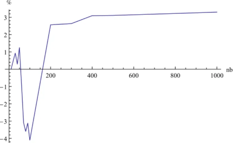
200 400 600 800 1000nb -4 -3 -2 -1 1 2 3 %

Figure 3: Comparison (in %) of DE with TDA-100k on different number of turbines.

200 400 600 800 1000nb 0.5 1.0 1.5 2.0 2.5 3.0 3.5 logHtimeL

Figure 4: TDA-100k (blue) and DE (red) execution time on different number of turbines. Scale is loga-rithmic in log₁₀(time).

In order to test our pattern modeling we used results previ-ously published by [9] on different wind farm sizes. Sev-eral scenarios were set up with varying numbers of bines, and varying farm sizes. For n = 10, 20, 30, ...100 tur-bines, a quadratic farm of size 3km × 3km was used, and for n = 200, 300, 400, 500 and 1000 turbines, rectangular farms of 8km × 5km, 10km × 6km, 12km × 6km, 14km × 7km and 20km × 10km were chosen.

Tables 1 and 2 compare results obtained using a Local Search algorithm proposed by Wagner in [9] to the patterns we optimized with a Genetic Algorithm(1) and a Differential Evolution Algorithm(2). These results are summarized for the DE algorithm in figures 3 and 4.

For each scenario, we executed 100 runs. In Table 1, the first columns give the size of the problem, the best and mean energy outputs in kW obtained by Wagner [9]. The compu-tation time in minutes for the 30 runs executed by Wagner is given in the fourth column. Columns 5 and 6 give the

n TDA 200k TDA 200k time GA GA GA time α δ gain(+)

Max Mean (min) Max Mean stdev (min) opt opt loss(-)

10 7.314e+04 7.309e+04 13 7.315e+04 7.314e+04 1.2e+01 6 810.14 0.495180 0.07% 20 1.449e+05 1.448e+05 30 1.456e+05 1.454e+05 1.5e+02 2 789.71 0.531091 0.41% 30 2.144e+05 2.135e+05 45 2.164e+05 2.162e+05 3.6e+02 2 746.27 0.038119 1.26% 40 2.806e+05 2.791e+05 61 2.814e+05 2.808e+05 1.9e+02 3 919.46 0.592378 0.61% 50 3.418e+05 3.412e+05 77 3.461e+05 3.461e+05 4.5e+00 3 745.07 0.737000 1.44% 60 4.022e+05 4.011e+05 95 3.988e+05 3.954e+05 4.7e+03 4 692.07 0.745209 -1.42 70 4.591e+05 4.555e+05 111 4.449e+05 4.443e+05 2.0e+03 5 566.51 0.726369 -2.46 80 5.108e+05 5.090e+05 129 4.925e+05 4.921e+05 9.3e+02 7 499.77 0.674266 -3.32 90 5.625e+05 5.609e+05 151 5.450e+05 5.419e+05 4.1e+03 7 431.46 0.725736 -3.39 100 6.113e+05 6.083e+05 170 5.863e+05 5.796e+05 7.2e+03 6 395.30 0.645553 -4.72 200 1.325e+06 1.323e+06 404 1.359e+06 1.359e+06 1.1e+01 16 727.00 0.688262 2.72% 300 1.973e+06 1.971e+06 678 2.025e+06 2.024e+06 1.5e+03 26 735.16 0.741059 2.69% 400 2.586e+06 2.584e+06 1020 2.666e+06 2.665e+06 4.0e+02 39 722.81 0.693413 3.13% 500 3.251e+06 3.249e+06 1470 3.352e+06 3.352e+06 3.4e+02 53 724.88 0.739885 3.17% 1000 6.454e+06 6.449e+06 4500 6.669e+06 6.668e+06 7.7e+02 166 709.31 0.694013 3.40%

Table 1: Comparison of results obtained with TDA and GA on different number of turbines (time is for 30 runs as in [9]).

n TDA 200k TDA 200k time DE DE DE time α δ gain(+)

Max Mean (min) Max Mean stdev (min) opt opt loss(-)

10 7.314e+04 7.309e+04 13 7.315e+04 7.313e+04 1.2e+01 6 809.93 0.495069 0.05% 20 1.449e+05 1.448e+05 30 1.456e+05 1.454e+05 1.4e+02 3 790.21 0.530879 0.41% 30 2.144e+05 2.135e+05 45 2.164e+05 2.164e+05 1.8e+02 3 745.82 0.038130 1.36% 40 2.806e+05 2.791e+05 61 2.814e+05 2.809e+05 2.2e+02 3 918.81 0.591977 0.64% 50 3.418e+05 3.412e+05 77 3.461e+05 3.460e+05 3.0e+01 3 744.85 0.736872 1.41% 60 4.022e+05 4.011e+05 95 3.988e+05 3.984e+05 3.9e+02 4 691.87 0.744932 -0.67% 70 4.591e+05 4.555e+05 111 4.449e+05 4.446e+05 2.2e+02 4 566.21 0.726147 -2.39% 80 5.108e+05 5.090e+05 129 4.924e+05 4.919e+05 2.6e+02 5 499.38 0.673879 -3.36% 90 5.625e+05 5.609e+05 151 5.450e+05 5.441e+05 5.6e+02 6 431.32 0.725975 -3.00% 100 6.113e+05 6.083e+05 170 5.862e+05 5.819e+05 2.2e+03 6 395.03 0.644272 -4.34% 200 1.325e+06 1.323e+06 404 1.359e+06 1.359e+06 1.1e+02 14 727.05 0.688215 2.72% 300 1.973e+06 1.971e+06 678 2.025e+06 2.025e+06 1.2e+03 23 735.13 0.741127 2.74% 400 2.586e+06 2.584e+06 1020 2.666e+06 2.664e+06 3.3e+02 35 722.76 0.693168 3.10% 500 3.251e+06 3.249e+06 1470 3.352e+06 3.350e+06 1.9e+03 50 724.75 0.739924 3.11% 1000 6.454e+06 6.449e+06 4500 6.669e+06 6.668e+06 6.8e+02 162 709.26 0.693959 3.40%

Table 2: Comparison of results obtained with TDA and DE on different number of turbines (time is for 30 runs as in [9]).

best and mean results obtained with our pattern with the Genetic Algorithm for 100 runs. Column 7 gives the stan-dard deviation of the results. Column 8 gives the mean time necessary for 30 runs, in order to compare the order of mag-nitudes with Wagner’s results. The time comparison itself is not very relevant, because the machines used are probably different, but the difference in magnitude (from 75 hours for n = 1000 with Wagner’s method to less than 3 hours with the GA approach) shows the impact of dealing with very few variables. Comparing the number of evaluations is much more relevant. In his paper Wagner, uses 200 000 eval-uations whereas the GA we implemented required only 4000 evaluations. The last column gives the gain(+) or loss(-) obtained on the mean value found with the GA compared to Wagner’s results.

Results show that for big farms (≥ 200 turbines) using a local search algorithm is less effective than optimizing the farm pattern. Surprisingly, this is also true for small farms (≤ 50 turbines). For mid-size farms the local search algo-rithm presented by [9] gives better results. This is consis-tent with results presented by Neubert [6]: for a 100 turbine farm, they obtained a 3% loss by using a regular pattern to optimize turbine positions.

Table 2 gives the same results for the DE approach and the conclusions are similar. This tends to show that the solution found is robust to the choice of the metaheuristic used. In bold we give the best results found for the two approaches.

5.

CONCLUSION

Optimizing wind farm configuration is a challenging issue for which problem modeling is critical. In this paper, we have shown that optimizing a simple pattern outperforms existing results on configurations involving a large number of turbines. The gain obtained for farms of 400 and more turbines exceeds 3%, while reducing computation time by an order of magnitude.

The modeling is deliberately simple, as this paper’s goal was to reduce as much as possible the number of variables of the general model while keeping excellent results: by reducing the size of the problem, we can focus on optimizing efficiently a small number of variables, and the loss due to the lack of generality of the model is more than compensated by a “better” optimization of the remaining variables.

There are now many directions for further research. On the one hand, this model can be complexified in order to create more elaborated shapes and to increase the variety of the solutions found. For example, we can imagine adding a number of homothetic deformations in the modeling. On the other hand these results can be used as a starting point for a single point optimization algorithm (such as simulated annealing or steepest descent) or to build a population of starting points for population based metaheuristics.

6.

REFERENCES

[1] Z. S. Andrew Kusiak, Haiyang Zheng. Power optimization of wind turbines with data mining and evolutionary computation. In Renewable Energy, volume 35, pages 695–702. Elsevier, 2010.

[2] J. S. Gonz´alez, M. B. Pay´an, J. M. R. Santos, and F. Gonz´alez-Longatt. A review and recent

developments in the optimal wind-turbine micro-siting problem. In Renewable and Sustainable Energy Reviews, volume 30, pages 133–144. Elsevier, 2014. [3] J. H. Holland. Adaptation in Natural and Artificial

Systems. University of Michigan Press, 1975.

[4] A. Kusiak and Z. Song. Design of wind farm layout for maximum wind energy capture. In Renewable Energy, volume 35, pages 685–694. Elsevier, March 2010. [5] G. Mosetti, C. Poloni, and B. Diviacco. Optimization

of wind turbine positioning in large windfarms by means of a genetic algorithm. In Journal of Wind Engineering and Industrial Aerodynamics, volume 51, pages 105–116. Elsevier, 1994.

[6] A. Neubert, A. Shah, and W. Schlez. Maximum yield from symmetrical wind farm layouts. In Proceedings of DEWEK 2010, the 10th German Wind Energy Conference, 2010.

[7] H. Neustadter. Method for evaluating wind turbine wake effects on wind farm performance. Journal of Solar Energy Engineering, 107:240–243, 1985.

[8] R. Storn and K. Price. Differential evolution - a simple and efficient heuristic for global optimization over continuous spaces. Journal of Global Optimization, pages 341–359, 1997.

[9] M. Wagner, J. Day, and F. Neumann. A fast and effective local search algorithm for optimizing the placement of wind turbines. In Renewable Energy, volume 51, pages 64–70. Elsevier, March 2013. [10] M. Wagner, K. Veeramachaneni, F. Neumann, and

U.-M. O’Reilly. Optimizing the layout of 1000 wind turbines. In European Wind Energy Association Annual Event, 2011.

[11] C. Wan, J. Wang, G. Yang, H. Gu, and X. Zhang. Wind farm micro-siting by gaussian particle swarm optimization with local search strategy. Renewable Energy, 48:276 – 286, 2012.

[12] C. Wan, J. Wang, G. Yang, and X. Zhang. Optimal micro-siting of wind farms by particle swarm optimization. In Advances in Swarm Intelligence, volume 6145 of Lecture Notes in Computer Science, pages 198–205. Springer Berlin Heidelberg, 2010. [13] F. Wang, D. Liu, and L. Zeng. Study on

computational grids in placement of wind turbines using genetic algorithm. In Proceedings of the World Non-Grid-Connected Wind Power and Energy Conference, 2009, pages 1–4. IEEE, 2009. [14] D. Wilson, E. Awa, S. Cussat-Blanc,

K. Veeramachaneni, and U.-M. O’Reilly. On learning to generate wind farm layouts. In GECCO ’13: Proceeding of the fifteenth annual conference on Genetic and evolutionary computation conference, pages 767–774, New York, NY, USA, 2013. ACM. [15] X. Yin and N. Germay. A fast genetic algorithm with

sharing scheme using cluster analysis methods in multimodal function optimization. In C. R.

R.F.Albrecht and N. Steele, editors, In proceedings of the Artificial Neural Nets and Genetic Algorithm International Conference, Insbruck Austria. Springer-Verlag, 1993.