Combinatorial Reverse Auctions in Construction Procurement

(1)

Combinatorial Reverse Auctions in Construction Procurement

Salim Al Shaqsi

Bachelor of Science, Mechanical Engineering, Queen’s University, 2009 SUBMITTED TO THE PROGRAM IN SUPPLY CHAIN MANAGEMENT IN PARTIAL FULFILMENT OF THE REQUIREMENTS FOR THE DEGREE OF

MASTER OF APPLIED SCIENCE IN SUPPLY CHAIN MANAGEMENT AT THE

MASSACHUSETTS INSTITUTE OF TECHNOLOGY JUNE 2018

The authors hereby grant to MIT permission to reproduce and to distribute publicly paper and electronic copies of this capstone document in whole or in part in any medium now known or

hereafter created.

Signature of Author……… Salim Al Shaqsi Master of Applied Science in Supply Chain Management Program May 11, 2018

Certified by……… Dr. Tugba Efendigil Research Scientist, Center for Transportation and Logistics Capstone Advisor

Accepted by………... Dr. Yossi Sheffi Director, Center for Transportation and Logistics Elisha Gray II Professor of Engineering Systems Professor, Civil and Environmental Engineering

(2)

Combinatorial Reverse Auctions in Construction Procurement By

Salim Al Shaqsi

Submitted to the Program in Supply Chain Management on May 11, 2018 in Partial Fulfillment of the

Requirements for the Degree of

Master of Applied Science in Supply Chain Management Abstract

Construction procurement often involves negotiations between many parties over multitudes of components. The process of allocating contracts to suppliers is generally a complex process involving multiple decision makers processing large amounts of information. Minimizing project costs while meeting stringent specification and schedule requirements is especially difficult. In most cases, procurement processes do not consider combinatorial (or package) bids from

suppliers. Allowing combinatorial bidding in the procurement process has been shown to reduce costs in other industries. It can, therefore, be expected to reduce costs in construction. This research proposes the use of combinatorial reverse auctions to minimize construction costs. Various models were applied to real data to determine feasibility compared to the baseline of allocating all items to the lowest bidder. Data included seven scenarios selected based on the number of suppliers and number of items. Each scenario included a subset of bids submitted by approved suppliers. A sensitivity analysis was performed on each model-scenario pair to consider uncertainty in supplier pricing structures. Results of the analysis provided justification for the use of combinatorial reverse auctions in construction procurements. Cumulative cost savings across all seven scenarios were 6.4% for unconstrained models and 2.7% for constrained models with limits on the number of awarded suppliers. Further analysis on the computation time and distribution of solutions across various methods indicated the superiority of the iterative approach to solving the winner determination problem in terms speed and optimality. However, stochastic and meta-heuristic approaches using a genetic algorithm led to higher variations in allocations while maintaining low variations in total cost. This suggests that they can be used to provide families of near-optimal solutions.

(3)

4.5.4. Model 4 – CRA with Non-linear Formulation ... 33 4.5.5. Summary of Models ... 34 4.5.6. Software Selection ... 34 5. Results ... 36 5.1. Scenario 1 ... 36 5.2. Scenario 2 ... 38 5.3. Scenario 3 ... 40 5.4. Scenario 4 ... 43 5.5. Scenario 5 ... 45 5.6. Scenario 6 ... 47 5.7. Scenario 7 ... 50 6. Discussion ... 52 7. Conclusion ... 54 8. References ... 55

List of Tables

Table 1: Auction Equivalencies ... 21

Table 2: Normalized cost matrix example ... 28

Table 3: Summary of Models ... 34

Table 4: Scenario 1 cost matrix ... 36

Table 5: Scenario 1 fixed costs ... 36

Table 6: Scenario 1 normalized cost matrix ... 37

Table 7: Scenario 1 discount rates ... 37

Table 8: Optimization and sensitivity analysis results of Scenario 1 ... 38

(5)

Table 13: Optimization and sensitivity analysis results of scenario 2 ... 40

(6)

(7)

7

1. Introduction

Due to ever increasing market competitiveness, construction companies face challenges in optimizing their supply chains. Specifically, managing the procurement of materials and services from multiple suppliers can be overwhelmingly complex. In other industries such as the transportation industry, more sophisticated approaches are used to assign contracts to suppliers. Combinatorial reverse auctions where suppliers are invited to bid on groups of items (or

packages) have been shown to offer significant savings. This project introduces various

approaches to optimizing procurement using combinatorial reverse auctions. Their performance is measured in terms of potential cost savings. Real data, provided by a sponsoring company, is used. The following sub-sections summarize the problem statement, the company background and the motivation for researching the proposed topic.

1.1. Problem Statement

Competitive market conditions have incentivized construction companies to build more efficient supply chains. There is a growing focus on improving procurement processes to lower construction costs while improving performance. Maintaining competitiveness involves having a broader perspective and analyzing the supply chain over a larger space and time horizon while planning for a variety of scenarios. It also involves translating the qualitative results into quantitative metrics that are descriptive, complete and intelligible across the firm. They should be designed to capture various supplier characteristics such as cost, quality, reliability, resilience and long-term risk. They should also be represented in common units (such as monetary units) for continuity and so that they can then be used in decision support systems to make more informed operational and short-term decisions. It is also vital that they be revisited and continually adjusted to reflect new data.

(8)

8 The procurement process, being a significant part of the operations of the firm, can be redesigned to consider market dynamics and supplier metrics to boost the firm’s short-term profitability and bolster its long-term growth potential. However, this does come at a complexity cost when increasing numbers of inputs and interactions of inputs are expected. The complexity issue can be mitigated by employing mathematical models and leveraging the exponentially growing computational power and software tools now abundantly available at low cost. If supplier metrics are designed correctly, software decision support tools can replace existing qualitative decision processes with ease. Procurement optimization using software tools would not only offer firms significant short-term and long-term savings, it would give them the opportunity to quantitatively define and document its procurement process and allow it to be adjusted more easily in the future.

An important aspect of suppliers’ cost structures, often overlooked by procurement teams in construction firms, is the importance of economies of scale and scope. Suppliers’ production cost structures often include fixed costs that are independent of the scale of production. This translates to lower costs (per item) of supplying larger numbers of items. Additionally, because of the inherently large uncertainty in demand within the construction industry, suppliers tend to favor larger contracts over smaller ones. This means that they would be in favor of offering volume-based discounts to increase their chances of maximizing contract revenue.

Reverse auctions (also referred to as tendering) are commonly used in construction procurement as a matchmaking process to select suppliers that best “fit” certain criteria. This is mainly done to minimize costs. The process is preceded by a detailed technical review of supplier proposals to ensure all participants in the auctions can deliver the products and services while meeting technical requirements. Contracts with suppliers often include multiple line items,

(9)

9 where each line item represents a component or group of components in a construction project. While a supplier may have the lowest total cost for supplying all items in a given contract, it may have overpriced a subset of the items relative to other suppliers. Another approach could involve assigning each item to the lowest bidder. This would minimize costs if suppliers’ pricing

structures were linear with respect to the number of items in a contract. But in most cases, they are non-linear. In some cases, suppliers may be willing to share their pricing function, which may make solving the supplier assignment problem more tractable. Another approach could involve asking suppliers to submit bids for every possible combination of items. This may seem reasonable with a small number of items, but the number of combinations grows exponentially such that a set of only 30 items would require each supplier to submit over one billion bids and 300 items would require more bids than there are atoms in the visible universe. Auctions that consider combinations of items where sellers are bidders and buyers are the auctioneers are defined as combinatorial reverse auctions. They have been used extensively in the transportation sector for the procurement of transportation services and have yielded up to 15% reduction in costs.

This capstone seeks to answer the question: Can combinatorial reverse auctions be used to reduce construction costs?

1.2. Company Background

Shaksy Engineering Services (SES) was established in 2009 and based in Muscat, Oman. It is an engineering/construction company that primarily serves as a main contractor in

construction projects. It has enjoyed steady growth since its inception and currently has over 1,000 employees and has delivered over US $200 Million in construction projects. At the core of the company’s mission is the ability to deliver high-quality work on-schedule. This has allowed

(10)

10 SES to position itself favorably in a market where high-profile projects were gaining popularity. Although initial projects involved industrial and utility buildings, recent projects include bank headquarters, hotels, cinemas and colleges where specifications call for higher build quality and demand high quality materials and good workmanship. As the company grows and expands to new markets, it seeks to standardize its business processes. It also plans to develop corporate strategies to overcome obstacles and threats while ensuring its core values are not compromised.

1.3. Motivation for Research

Construction activities make up a significant fraction of the global economy and are expected to grow significantly over the next decade. According to data from Trading Economics (2017), the construction industry makes up 4.8% of the US gross domestic product (GDP) and 6.3% of China’s GDP. A report by Global Construction Perspectives and Oxford Economics forecasts that the volume of construction output will grow by 85% to US $15.5 trillion

worldwide by 2030. As emerging market economies such as Oman have been easing regulations to attract foreign investment, an influx of new construction companies has been seen throughout the country. New companies include locally owned and foreign owned businesses, the latter having greater leverage due to existing reputation and greater purchasing power. While projects may have been plentiful (to each company) in the past, they have become scarcer due to the influx of these newcomers. In addition to this, declining oil prices (Figure 1) have led to an economic recession in the region. Following adverse economic conditions, companies in the region are adopting leaner business models to cut waste and mitigate losses. Companies are also increasingly turning to software solutions to consolidate and analyze data while utilizing decision support systems to drive profitability. Procurement software systems coupled with sophisticated auction design can lower costs and give companies a competitive advantage.

(11)

11 Figure 1: Oil Prices 2013-2017. Source: Infomine.com

(12)

12

2. Literature Review

To cover theoretical models as well as practical approaches, this review includes three areas related to the subject as follows; current best practices and market trends in construction procurement defined by leading professional industry bodies and international consultant firms; applications of reverse auctions and combinatorial reverse auctions in various industries; mathematical models and winner-determination algorithms.

2.1. Current Best Practices and Market Trends

This section summarizes the body of knowledge on construction procurement amassed by professional industry bodies and industry experts.

The Chartered Institute of Building’s report (2010) exploring procurement in the construction industry surveyed 525 construction industry professionals in the United Kingdom. A large majority of the respondents (82%) believed that “suicide bidding” (the practice of bidding unusually lower than competitors to obtain work even at a financial loss) exists within the industry. The report recommended that procurement teams should not select suppliers purely based on cost, unsustainable bids should be identified and rejected. The negative effects of suicide bidding were reported to be felt throughout the supply chain, with upstream and

downstream stakeholders experiencing schedule disruptions and financial losses. The report also highlighted the prevalence of cover pricing, which is a form of bid-rigging where suppliers submit inflated bids with the aim of not securing the contract. Hughes (2017) reported a trend of low-margin pricing among suppliers during periods of adverse economic conditions and scarcely available work. Suppliers forwent considering risks in their cost structures and attempted to enhance their revenues though variations (changes made to a project post award). This often led to conflicts between buyers and suppliers during the delivery of projects.

(13)

13 The building and construction procurement guide of Australia (2014) and the

construction procurement policy framework of Northern Ireland (2017) stressed the importance of ensuring suppliers can carry out the required work. Both guides presented a framework for prequalification and advised limiting the number of suppliers to those that have met pre-specified commercial and technical criteria. An interactive and collaborative process between the client and suppliers was recommended for large-scale projects to enhance transparency and exchange of information. The process involves interviews and/or workshops to clarify contract scopes and required documentation.

Kent, Van den Berg and Sobolewski (2017) reported an increase in competitiveness among construction firms and a shift towards the use of lump-sum, turnkey (LSTK) contracts where firms bear the project cost and risk (lump sum) and guarantee operational readiness (turnkey). This practice has become commonplace in industrial and utility projects. However, some firms were still not effectively factoring contingency costs into their bids. Another trend reported by Kent et al. involved clients breaking up larger projects into smaller discrete elements. This was done to lower costs but often led to increased project management requirements and controls for dealing with a larger set of suppliers.

2.2. Reverse Auction Applications

During the rise in popularity of e-procurement in the 2000s, Wamuziri and Ab-Shaaban (2005) studied the advantages and disadvantages of using online reverse auctions in construction procurement. Advantages listed included increased efficiency, transparency and reduced costs. Disadvantages included awarding contracts to the lowest bid rather than the best value and difficulties in exercising control over specification for the goods and services being procured in complex projects. In an exploratory study of business to business (B2B) marketplaces, Minier

(14)

14 (2003) found that B2B exchanges (including e-auction sites) should be fair and accessible by all trading members regardless of size or duration of membership. The importance of transparency and integrity in rulesets was stressed, and it was recommended that all transactions made on an exchange should be reported promptly with full details on price and volumes.

Focusing on bidding strategies in online reverse auctions for automotive parts, Lopez (2000) found that larger suppliers were often earliest to bid and placed more conservative bids during auctions. They also did not engage in price wars with smaller suppliers. Smaller suppliers, on the other hand, would bid far more frequently and engaged in “bidding frenzies” (placing fractionally lower bids frequently) towards the end of auctions. Results implied larger suppliers had an a priori valuation, whereas smaller suppliers were more concerned with having the lowest bid. Similar trends were found between incumbent and new suppliers, indicating bidders with more experience often perform better when participating in online reverse auctions.

In the transportation sector, Sheffi (2004) concluded that many large firms used

combinatorial reverse auctions for the procurement of truckload transportation services achieving cost savings between 3% and 15%. Combinatorial bidding on sets of shipping lanes allowed both shippers and suppliers to exploit inherent economies of scope. Shippers also enjoyed higher service levels by adjusting supplier bids based on various factors, such as on-time performance, ease of doing business, familiarity with the shipper’s operations and availability of the right equipment. Additional system constraints were often used to reflect business rules specified by the shipper. Constraints included lane/facility requirements, supplier volume of business requirements, supplier capacity constraints and quota constraints. Noncompeting shippers were found to participate in joint procurement, further increasing economies of scope, as their shipping lanes were often complementary.

(15)

15 Lunander and Lundberg (2012) analyzed the results of public procurement in Sweden using first-price sealed bid combinatorial reverse auctions. The procurement of various public services was included in the analysis including (but not limited to) road resurfacing, cleaning services and domestic flights. Compared to only considering single-item bids, allowing package bids reduced costs by up to 5%, with an average cost reduction of 2.4%. Distribution of awarded contracts among suppliers was higher when considering package bids, and a positive correlation between the number of items and number of bidders was found.

In terms of practical considerations in auction design, Sheffi (2003) compared the advantages and disadvantages of both sealed and open bid auctions. Sealed bid auctions tended to attract more bidders and deter predatory behavior (larger suppliers lowering their bids to such low levels that smaller supplier cannot compete) and collusion between them. However, the lack of transparency allowed the potential for the auctioneer to change rules after bidding or offer unfair preferential treatment to certain bidders without other bidders’ knowledge. On the other hand, open bid auctions offered more transparency and were less open to manipulation by the auctioneer. However, they were more susceptible to collusion and predatory bidding. In multi-item auctions, open formats had the added disadvantage of allowing bidders to drive down prices on specific items that other bidders were most interested in. Sheffi also listed additional

important criteria to be considered during reverse (procurement) auctions, such as efficiency, robustness, simplicity and speed. Because of this, most procurement departments preferred sealed bid first price auctions over other types of auctions. Long term relationships between buyers and sellers (auctioneers and bidders) were common in reverse auctions in B2B settings. This often led to implications such as sequential (repeating) auctions, asymmetric information among bidders, and aggregation of information among auctioneers.

(16)

16

2.3. Mathematical Models

Using simulated bids, Andersson et al. (2000) compared computation times of different algorithms for solving the winner-determination problem in simple combinatorial auctions (only single units of a commodity are traded, and no supplier constraints are used). Under most bid distributions, integer programming (IP) formulations using IBM’s CPLEX solver performed well compared to other algorithms such as the combinatorial auction structured search (CASS)

algorithm and Sandholm’s algorithm. However, when a binomial distribution was used to construct bids, the CASS algorithm outperformed CPLEX by a significant amount. Based on these results, a simple enumeration algorithm that outperformed CASS under such bid

distributions was proposed. It was concluded that CPLEX was the most versatile algorithm and had the added benefit of being able to solve more complex combinatorial auctions with multiple units per commodity, non-zero reserve prices and additional side constraints.

Caplice and Sheffi (2005) defined various mixed-integer programming (MIP)

formulations for the winner determination problem (WDP) in combinatorial reverse auctions for the procurement of truckload transportation. The simplest formulation minimizes cost without side constraints. Subsequent models add additional constraints to reflect business rules, such as business guarantee constraints, supplier base size constraints, soft constraints and “If then” constraints. Following a study of bidding behaviors among various suppliers in such auctions, Ueasangkomsate and Lohatepanont (2012) proposed a linear programming (LP) model formulation for suppliers to determine package bid-to-cost ratios that maximize profit.

Results from a comparative study by Hsieh and Huang (2010) indicated that combinatorial reverse auctions based on group buying outperform multiple independent combinatorial reverse auctions in terms of both cost minimization and computation time. A

(17)

17 specialized heuristic algorithm based on Lagrangian relaxation was used in both cases to solve the winner determination problem using simulated data.

In an analysis of iterative combinatorial auctions, Parkes (2006) categorized model design in terms of design features such as timing rules, information feedback, bidding rules, termination conditions and bidding language. Various models were analyzed, including common price-based models where ask prices are provided to bidders before each round as well as less common non-price-based models. The study concluded that a tradeoff exists between the cost of eliciting information (from bidders) and the value of additional information in terms of

improving the market allocation.

Hsieh (2010) proposed a novel approach for giving feedback to bidders participating in iterative combinatorial auctions without revealing as much information as revealing winning bids or ask prices at each iteration. The model adopts Lagrangian relaxation techniques used in other models to reveal Lagrangian multipliers to bidders. Each bidder then solves a profit-maximizing LP model to determine whether to submit a new bid. A heuristic algorithm was proposed for solving the WDP at the end of the last bidding round.

(18)

18

3. Auction Theory

The following section is a summary of the body of knowledge on auction theory. It is intended to give the reader a brief introduction to the subject and offer some insights into auction design and common types of auctions used in practice. The section is a summary of existing work compiled by Sheffi (2003).

An auction is a mechanism where an auctioneer is either looking to buy or sell a set of goods and/or services. The selection and payment mechanisms are determined based on bids received. A simple example is real-estate auctions where auctioneers sell houses or buildings to the highest bidders. Reverse auctions are equivalent with the caveat that auctioneers are the buyers who seek to minimize cost rather than maximize it. Reverse auctions are commonly used in business settings for the procurement of goods and services. Most buying or selling

transactions where more than two parties are involved can be considered auctions. In fact, auctions are often thought to be the most economically efficient way of distributing resources. They have been in use for millennia throughout history. For the sake of brevity, this section will only consider auctions in which the seller is the auctioneer.

Auctions are designed to serve three main purposes:

 Price discovery: Determining the true pricing of a product or service.

 Winner determination: Determining the winner (usually the highest bidder) of the auction.

 Payment mechanism: Determining the price that should be paid by the winner.

(19)

19  Revenue: Maximizing revenue is the primary objective of the auctioneer in most cases.

However, this is not always the case. Other considerations and constraints, such as risk control, may be just as important.

 Efficiency: A measure of whether bidders with the highest valuation ex post are selected. This is especially important when the delivery of the good or service will occur in the future.

 Time and Effort: Auctions should ideally be designed to minimize the effort required by the auctioneer and bidders. Complicated auctions involving multiple items and multiple rounds of bidding often have a high data, computation and communication complexity.  Simplicity: Building off the previous point, overly complicated auctions may deter

participants who do not fully understand the rules. Keeping the rules simple is an important aspect of auction design.

Bidder valuations can be categorized in to three different categories:

 Private values (PV): Each bidder only knows its own valuations and they are not affected by other bidders’ valuations.

 Interdependent values: The valuation is partially known by bidders but may change based on signals from other bidders.

 Common values: The valuation is the same for all bidders (ex post).

3.1. Common Types of Auctions 3.1.1. Open bid auctions

Open bid auctions are auctions where all bidding information is accessible by all bidders. Therefore, all bidders know what bids were placed. The following are some of the common types of such auctions used in practice:

(20)

20  Ascending bid auction (English auction), where the price is raised by bidders continually

until only one bidder remains. This bidder wins the auction and pays the final price.  Descending bid auction (Dutch auction) where the price is lowered by the auctioneer

starting from a high price. The first bidder that accepts a price wins paying the last price quoted.

 Ascending clock auction (Japanese auction) where the auctioneer continually raises the price until only one bidder remains. Once a bidder exits, they are not allowed to re-enter and will lose their chance of winning the auction.

3.1.2. Sealed-bid auctions

Sealed-bid auctions are auctions where bidding information is not shared with all the bidders. A bidder only knows what he/she bid and not what others have bid. The following are common sealed-bid auction types:

 First price sealed bid auction where each bidder submits a confidential bid. The highest bidder wins and pays the amount they bid

 Second price sealed bid auction (Vickery auction), which is identical to the first price auction, but the winner pays the amount bid by the second highest bidder.

The important difference between open bid and sealed-bid auctions is that information feedback is not given to bidders in sealed-bid auctions. There are auctions that reveal partial information such as bidder rankings so that a bidder can know his current standing (first, second, third, etc.) and other bidders’ standings but not bid values.

There are important game theory-based insights from the auction types listed above. For example, a winning bid in a first price sealed-bid auction is equivalent to a winning bid a

(21)

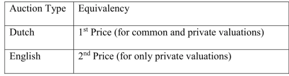
21 descending bid (Dutch) auction. This is because none of the bidders in a Dutch auction has any information until a winner is selected. But this is only the case if the auction is not repeated or an auction with a similar item is not subsequently held. Table 1 summarizes the equivalencies between open and sealed-bid auctions.

Auction Type Equivalency

Dutch 1st_{Price (for common and private valuations)}

English 2nd_{Price (for only private valuations)}

Table 1: Auction Equivalencies 3.2. Bidding Strategies and Auction Revenues

Based on the type of auction, bidders may want to define their strategy before the auction to maximize their utility. Conversely, auctioneers may want to design the auction based on the outcome that is preferable to them. The following assumptions will be held throughout this subsection:

 All bidders follow the same strategy resulting in Nash equilibrium.

 Bidders’ (private) valuations are independently and identically distributed (symmetric).  Bidders are risk neutral and therefore do not participate in collusion or predatory

behavior.

 Bidders have no budget constraints.

3.2.1. First Price Strategy and Revenue

A bidder in a first price sealed-bid auction seeks to maximize his/her expected gain. The expected gain is the probability of winning 𝑃(𝑏) times the surplus attained given a bid 𝑏 and valuation 𝑣 as shown in Equation 1.

(22)

22 𝐸[𝐺𝑎𝑖𝑛] = (𝑣 − 𝑏)𝑃(𝑏) [1]

It has been shown that for maximizing expected gain given 𝑛 bidders and a uniform distribution 𝑈[0,1], the optimal bid is shown in equation 2.

𝑏∗ ₌𝑛 − 1

𝑛 𝑣 [2]

Given this bid distribution and bidder strategy, the auctioneer can expect a revenue of:

𝐸[𝑅𝑒𝑣𝑒𝑛𝑢𝑒] =𝑛 − 1 𝑛 + 1 [3]

3.2.2. Second Price Strategy and Revenue

In a second price auction, the dominant strategy for a bidder is to bid their true valuation. This is because there is no additional surplus in bidding higher or lower than the true valuation. If all bidders follow this strategy, the expected revenue is equivalent to the first price revenue shown in equation 3. The equality is known as the revenue equivalence theorem. In fact, it holds true for any bid distribution given the assumptions listed in Section 3.2.

3.3. Practical Considerations in Procurement

In the context of procurement (or reverse) auctions, the focus shifts from allocation efficiencies mentioned in previous sections to simplicity. Most business to business reverse auctions are based on the first price sealed bid format (or a variant of it). The simplicity of the auction is attractive to both auctioneers and bidders and often involves a minimal number of bidding rounds.

(23)

23

4. Methodology

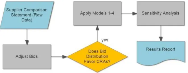
The methodology section outlines the mathematical and logical framework for implementing combinatorial reverse auctions (CRAs) in construction procurement. Figure 2 depicts the methodology steps that start with leveraging items based on various number of suppliers and items, and cost values. After aggregating the line-items into item groups, package generation and optimization model are applied. The methodology ends with a sensitivity analysis to compare the effects of different scenarios.

Figure 2: Methodology Outline

Data used in the study was provided by Shaksy Engineering Services LLC (SES). They also provided relevant information regarding market dynamics and supplier characteristics. The identity of suppliers will remain anonymous and will be referred to categorically (Supplier 1, Supplier 2 etc.). All monetary values (costs) are in Omani rials (OMR).

The simplest form of a CRA can be defined as an auction that allows bidders to submit bids on any subset of a list of items. The objective is to minimize the total cost while ensuring all

(24)

24 items are purchased. Or, more formally, given a universe of 𝑛 items 𝐼 = {𝑖 , 𝑖 , ⋯ 𝑖 } and a family of 𝑚 subsets of 𝐼, 𝑃 = {𝑝 , 𝑝 , ⋯ 𝑝 } with costs 𝑐 associated with each set in 𝑆, find the minimum cost subset 𝑃′ ⊆ 𝑃 such that the union of all sets in 𝑃′ equals 𝐼. This definition

assumes free disposal. Without free disposal an extra requirement that all sets in 𝑃′ be disjoint would need to be added. Free disposal (the auctioneer can freely dispose of excess production factors) was assumed throughout this project.

The problem is mathematically identical to the weighted set cover problem and is therefore considered NP-Hard. Because the weighted set cover problem is well studied in computer science spheres, many solver algorithms exist including a variety of potent heuristic algorithms that run in polynomial time.

Given the scale of the data and the complexity of the proposed models, integer

programming (IP) and non-linear formulations were selected for use on this project due to the effectiveness, robustness and popularity of available commercial solvers. IP solvers also add more flexibility in adding constraints to the model to reflect business rules. Such constraints are not as easily implemented in more specialized algorithms.

4.1. List of Symbols

𝑍: Objective function [OMR] 𝑥: Package selection binary variable 𝑦: Supplier selection binary variable 𝑖: Item index

𝐼: Set of all items in a scenario 𝑝: Package bid index

(25)

25 𝑃: Set of all packages in a scenario

𝑃’: Winning set of packages 𝑆’: Winning set of suppliers 𝑠: Supplier index

𝑆: Set of all suppliers within a scenario 𝑘: Project index

𝐾: Set of all projects to be analyzed 𝐶: Bid cost [OMR]

𝐹: Supplier fixed cost [OMR] 𝑇: Item/supplier cost matrix [OMR] 𝑇∗_: _{Normalized item/supplier cost matrix}

𝑄: Item/package binary matrix 𝑅: Supplier/package binary matrix 𝑀: Number of items in a scenario

𝑆 : Maximum allowable number of suppliers selected per section 𝑆 : Minimum allowable number of suppliers selected per section 𝐷: Discount value [OMR]

𝑑: Discount rate based on supplier revenue [%/OMR] 𝐵: Failure cost [OMR]

𝑒: Supplier performance rating on a given project and item 𝐸: Aggregated supplier performance rating

(26)

26 4.2. Segmentation

Construction project bills of quantities (BOQs) often include multiple bills and multiple sections within each bill representing related groups of line items. The BOQ data structure is depicted in the entity relationship diagram (ERD) in Figure 3.

Figure 3: Bill of quantities entity relationship diagram

Suppliers generally submit bids consisting of items contained in one bill (section) without overlap into other bills. Because of this, a (CRA) can be held for each bill independently. This has the added benefit of reducing the data and computational complexity as it exponentially reduces the number of possible packages relative to the number of possible packages over the entire BOQ.

A decision rule was used to select sections of various project BOQs to be used in the auctions. The rule required a minimum budgeted cost and minimum number of suppliers for each section. This rule reflects the Kraljic segmentation strategy to identify leverage items favorable to reverse auctions. Individual line items were aggregated into groups based on item

(27)

27 relationships. They were also aggregated based on a minimum (budgeted) cost per group. This is done because suppliers will generally not bid on an individual item if the value is too low or if it is too closely related to other items in a section.

4.3. Data Analysis

The data provided by SES included supplier comparison statements exported from their ERP system in Excel format. The statements include the following:

 Item descriptions and quantities

 Budgeted unit rates and amounts for each item

(28)

28 Examples of items included in comparison statements include raw materials,

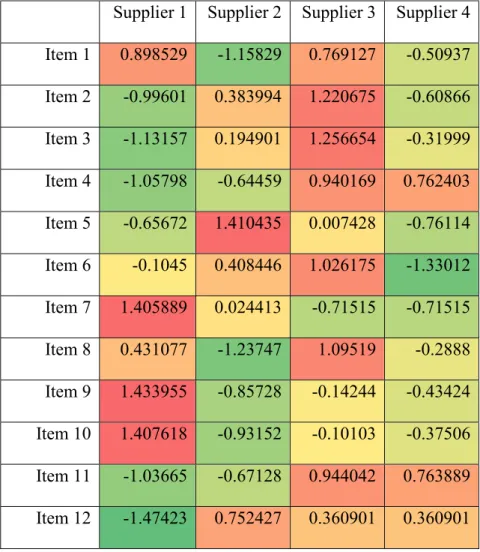
electrical/mechanical components and labor. The comparison statements were split into groups of related items. Data from each statement was used to generate an item/supplier cost matrix 𝑇. The cost matrices were modified by aggregating items into groups as described in Section 4.2. Each row in a given cost matrix represents an item group. The rows were then normalized

(subtracted by the mean and divided by the standard deviation) and stored in a normalized matrix 𝑇∗_{. An example of such a matrix is shown in Table 2.}

Supplier 1 Supplier 2 Supplier 3 Supplier 4 Item 1 0.898529 -1.15829 0.769127 -0.50937 Item 2 -0.99601 0.383994 1.220675 -0.60866 Item 3 -1.13157 0.194901 1.256654 -0.31999 Item 4 -1.05798 -0.64459 0.940169 0.762403 Item 5 -0.65672 1.410435 0.007428 -0.76114 Item 6 -0.1045 0.408446 1.026175 -1.33012 Item 7 1.405889 0.024413 -0.71515 -0.71515 Item 8 0.431077 -1.23747 1.09519 -0.2888 Item 9 1.433955 -0.85728 -0.14244 -0.43424 Item 10 1.407618 -0.93152 -0.10103 -0.37506 Item 11 -1.03665 -0.67128 0.944042 0.763889 Item 12 -1.47423 0.752427 0.360901 0.360901

(29)

29 4.4. Bid Adjustments

Bid adjustments were applied in a similar fashion to the adjustments described in Sheffi (2004). The bid values which are included in the provided comparison statements are already adjusted for cost of capital (due to payment terms), transportation costs, costs due to deviations from the technical specifications, installation costs and operations and maintenance costs. The following sections will present bid-adjustment methods used by SES as well as additional recommended methods.

4.4.1. Logistics Costs

The logistical costs can be split into transportation and inventory holding costs. Where transportation to site is not included in quotes, transportation costs are estimated based on previous rates for similar items and routes. If no data exists on previous routes, a transportation cost is applied based on the volume and weight of the item and distance traveled [OMR/kg/m or OMR/m3_/m].

Inventory holding costs are more complex because they depend on when ownership transfer occurs, where inventory is physically stored, the storage requirements and the duration of storage. Inventory holding costs are currently not considered in bid adjustments. A fixed inventory carrying rate [OMR/OMR/week] was recommended for future projects and not

considered for the purposes of this project as they are not expected to change significantly across suppliers.

4.4.2. Costs Due to Deviations from Specification

Construction project technical specifications tend to be very detailed and include many requirements. Supplier bids that partially match the specifications are sometimes accepted with the hope to be approved by the project client (building owner(s) or their representatives).

(30)

30 However, deviations from the design due to alternative products/materials are common in such cases and the cost of deviation is calculated based on the required modifications. This is also sometimes estimated as a percentage of the item cost. Installation costs are estimated in a similar manner where applicable.

4.4.3. Operation and Maintenance Costs

When procured items include the supply and or installation of machinery, operation and maintenance costs are usually included in bids. Where such costs are not included in bids, a cost is added based on quotes from other suppliers or estimated based on previous project costs.

4.4.4. Fixed Costs

High value bids will sometimes include a fixed cost (often called a preliminary cost). This cost is incurred by the company if the supplier is selected (regardless of the number items included in the contract). Additional indirect fixed costs were added to reflect the cost of doing business with each supplier.

4.4.5. Cost of Capital

The costs were adjusted for the cost of capital. This is done using the internal monthly discount rate 𝑟 usually specified by the accounting/finance department and supplier payment term duration 𝑡 expressed in months after the expected issue of the purchase/work order as shown in Equation 4.

𝐶∗ = 𝑐

(1 + 𝑟) [4] 4.4.6. Selection of Items & Scenarios

The selection process involved selecting scenarios that contain more than two suppliers and more than five aggregated items. The item supplier matrices were further analyzed to select

(31)

31 the scenarios that would benefit most from CRAs. This was achieved by filtering out scenarios where one supplier has the lowest bid across more than 80% of the items in a scenario.

4.5. Mathematical Model Formulations

The following sections describe the model formulations used in this project. The four models cover applications of CRAs under different scenarios.

4.5.1. Model 1 – Baseline

Model 1 is the integer programming (IP) formulation with minimal constraints. It is equivalent to the model described in Andersson, Tenhunen, & Ygge (2000). The model does not distinguish between bidders (suppliers) and is designed to benchmark various solvers and provide fast insights into the feasibility of CRAs. The model takes adjusted supplier bid costs 𝑐 and included items in each bid as inputs. The included items in each bid were converted into binary vectors (packages) and combined into an item/package binary matrix 𝑄. As the data is expected to include only a handful of package bids with more than 1 item, pricing was estimated based on applying a revenue-based discount 𝑑. Package bid values were calculated based on the single item bids. For a given subset of items 𝐼′ ⊆ 𝐼 with single item bid values 𝑐 , ∀𝑝 ∈ 𝑃 where 𝑃 is the set of single item bids, a package bid cost was calculated as shown in Equation 5.

𝑐 = 𝑐

∈

1 − 𝑑 𝑐

∈

[5]

A subset of bid package vectors 𝑄′ were generated stochastically using the normalized item/supplier cost matrix (Equation 6).

𝑄_, = −𝑁 𝑇∗_, + ℛ + 1 , ∀𝑖 ∈ 𝐼 [6]

𝑁 is the standard normal cumulative distribution function and ℛ is a randomly generated number (between -0.5 and 0.5). The set of packages were concatenated onto the item/package

(32)

32 matrix 𝑄. This process was repeated while pruning duplicate vectors until a reasonable number of packages was achieved or a pre-set computation time limit was reached. Each package was then duplicated for each supplier. The IP formulation is shown in Equations 7.1 and 7.2. argmin 𝑍(𝑥) = 𝑐 𝑥 [7.1]

𝑠. 𝑡 𝑄_, 𝑥 = 1, ∀𝑖 ∈ 𝐼 [7.2]

4.5.2. Model 2 – CRA with Supplier Constraints

Model 2 builds on Model 1 and includes supplier-wise constraints as described in Caplice & Sheffi (2005). The model captures complexity costs associated with interacting with multiple suppliers and corporate strategies in supplier selection. The model used the same data as Model 1 and included the same generated packages. To capture the direct and indirect costs of managing suppliers, a fixed cost for each supplier was included in the formulation. Minimum and

maximum numbers of suppliers were added as hard constraints to reflect the corporate strategy. The IP formulation for Model 2 is shown in Equations 8.1–8.6.

argmin 𝑍(𝑥, 𝑦) = 𝑐 𝑥 + 𝑓 𝑦 [8.1] 𝑠. 𝑡 𝑄_, 𝑥 = 1, ∀𝑖 ∈ 𝐼 [8.2] 𝑅 , 𝑥 − 𝑀𝑦 ≤ 0, ∀𝑠 ∈ 𝑆 [8.3] 𝑆 ≤ 𝑦 ≤ 𝑆 [8.4] 𝑥 ∈ {0,1}, ∀𝑝 ∈ 𝑃 [8.5] 𝑦 ∈ {0,1}, ∀𝑠 ∈ 𝑆 [8.6]

(33)

33 4.5.3. Model 3 – Iterative CRA

Model 3 is a simulation of an iterative auction process Parkes (2006) which begins with suppliers submitting single item bids. The auctioneer then analyzes the bids and proposes

packages to suppliers. Package bids that are received from suppliers are then analyzed to produce new package recommendations. This process is repeated for a pre-defined number of iterations or until the solution converges.

The IP formulation is identical to Model 2 and used the winning set of packages 𝑃 on a given iteration as package proposals for the next iteration. The discount function defined in Equation 4 was used on proposed packages to simulate supplier discounts. The model was initialized by solving the IP with single item bids only.

4.5.4. Model 4 – CRA with Non-linear Formulation

In this model, the discount function is included in the objective function. This drastically reduces the number of decision variables as only single-item bids are considered. However, since the objective function involves quadratic terms in 𝑥 and 𝑦, the problem is no longer linear and was solved using a genetic algorithm solver. The formulation is shown in Equations 9.1–9.6.

argmin 𝑍(𝒙, 𝒚) = 𝑐_, 𝑥_, − 𝑑 𝑐_, 𝑥_, + 𝑓 𝑦 [9.1] 𝑠. 𝑡 𝑥_, = 1, ∀𝑖 ∈ 𝐼 [9.2] 𝑥_, − 𝑀𝑦 ≤ 0, ∀𝑠 ∈ 𝑆 [9.3] 𝑆 ≤ 𝑦 ≤ 𝑆 [9.4] 𝑥_, ∈ {0,1}, ∀𝑖 ∈ 𝐼, ∀𝑠 ∈ 𝑆 [9.5] 𝑦 ∈ {0,1}, ∀𝑠 ∈ 𝑆 [9.6]

(34)

34 4.5.5. Summary of Models

Table 3 summarizes the four models proposed in this project.

Model Description Reason for use Expected Pros Expected Cons 1 Baseline

CRA

Test various solvers and benchmark performance of other models

Easiest to solve and can be solved using a variety of solvers

Doesn’t differentiate between suppliers and doesn’t model fixed costs

2 CRA with

supplier constraints

Model supplier fixed costs and constraints

Faster to solve than subsequent models if a limited number of packages are used

Will usually not find a better solution than subsequent models if packages are sparse 3 Iterative CRA Better simulate real

auctions where bidding is limited and doesn’t take place simultaneously

More realistic and has the potential to converge to a better solution than previous models on auctions with many items and suppliers

May take longer to solve since the IP solver will be run on every iteration

4 Non-linear

Model Including the pricing function in the objective function allows the solver to search over the entire allocation space

Reduction in number of decision variables and does not require package bids as inputs

Involves solving a non-linear objective function and may not be feasible for larger auctions

Table 3: Summary of Models

4.5.6. Software Selection

Given the selection of IP formulations, a multitude of software solutions were available for selection (for Models 1-3). Google Ortools was chosen because of its good performance, its availability as a free software and its ability to run as a package within Python. For Model 4, a genetic algorithm written in Python was used. The genetic algorithm was chosen over more specialized quadratic programming solvers because of its ability to consider any cost or discount

(35)

35 function. It also has the ability of producing a family of solutions whereas other solvers only provide one.

4.5.7. Sensitivity Analysis

To measure the robustness of each model, a sensitivity analysis was conducted on all models. The analysis involves running Monte Carlo simulations by repeatedly picking discounts rates from a triangle distribution and solving the models to generate a distribution of solutions. The distribution of the allocation matrices and total costs were analyzed. The coefficient of variance (CV) of the total cost and average CV of the allocation matrices was reported to

indicate the sensitivity of the models to uncertainty in discount rates. The methodology flowchart is shown in Figure 4.

(36)

36

5. Results

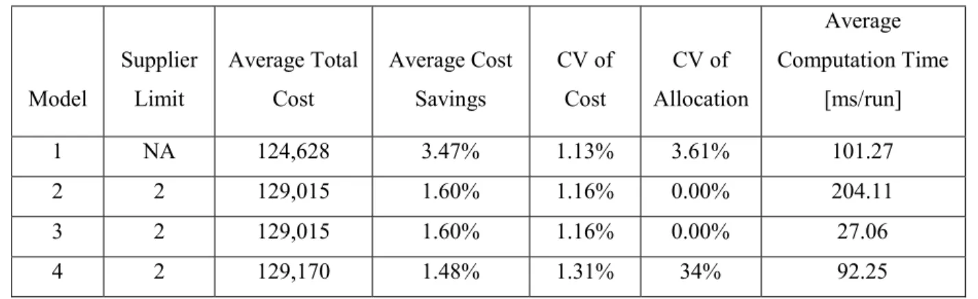
5.1. Scenario 1

Scenario 1 included bids from three suppliers. The scenario includes material and labor costs and originally consisted of 40 line-items. The scenario was aggregated into seven items. The cost matrix is shown in Table 4.

Supplier 1 Supplier 2 Supplier 3

Item 1 20608.5 23428 20453 Item 2 1377 855 1294 Item 3 88569 89400 106478.2 Item 4 3000 589 1700 Item 5 3559 5142 2965.9 Item 6 6750 4904 7200 Item 7 9550 NA NA

Table 4: Scenario 1 cost matrix

Fixed costs were determined based on indirect costs associated with coordinating with suppliers and are shown in Table 5.

Fixed Cost Supplier 1 2000 Supplier 2 2000 Supplier 3 2000 Table 5: Scenario 1 fixed costs

(37)

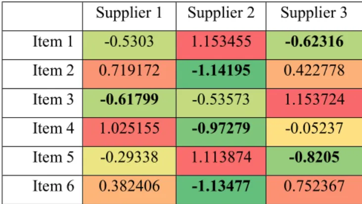
37 The normalized cost matrix is shown in Table 6 (for Items 1–6):

Supplier 1 Supplier 2 Supplier 3 Item 1 -0.5303 1.153455 -0.62316 Item 2 0.719172 -1.14195 0.422778 Item 3 -0.61799 -0.53573 1.153724 Item 4 1.025155 -0.97279 -0.05237 Item 5 -0.29338 1.113874 -0.8205 Item 6 0.382406 -1.13477 0.752367

Table 6: Scenario 1 normalized cost matrix

The data shows significant variations in costs between suppliers despite their total costs being similar. This would indicate that optimization could yield a better allocation than the baseline.

Discounts rates applied to each supplier were sampled from a triangular distribution and are shown in Table 7 (all values are in %/100k OMR).

Supplier Min Mode Max

1 0 2.46% 4.92%

2 0 0.82% 1.64%

3 0 0.82% 1.64%

(38)

38 The results of the optimization runs (including sensitivity analysis) are shown in Table 8.

Model Supplier Limit Average Total Cost Average Cost Savings CV of Cost CV of Allocation Average Computation Time [ms/run] 1 NA 124,628 3.47% 1.13% 3.61% 101.27 2 2 129,015 1.60% 1.16% 0.00% 204.11 3 2 129,015 1.60% 1.16% 0.00% 27.06 4 2 129,170 1.48% 1.31% 34% 92.25

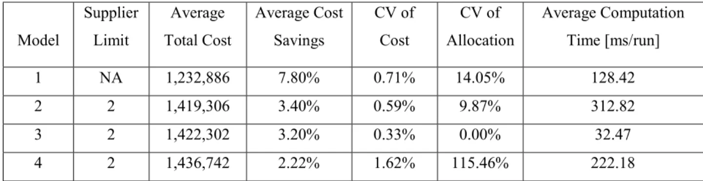
Table 8: Optimization and sensitivity analysis results of Scenario 1 5.2. Scenario 2

Scenario 2 included bids submitted from three. The scenario included 10 items

aggregated from 265 line-items. The cost matrix is shown in Table 9 (lowest bids are in bold).

Item 1 51449 35453 18134 Item 2 145210 161410 131625 Item 3 183645 181950 174669 Item 4 313966 188248 169605 Item 5 518961 538967 534460 Item 6 217598 170095 170129 Item 7 3136 1356 2806 Item 8 4063 1551 2753 Item 9 59566 73033 30501 Item 10 50295 33813 147057

(39)

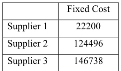
39 Fixed costs were provided by suppliers based on their preliminary costs (setup costs) and are shown in Table 10.

Fixed Cost Supplier 1 22200 Supplier 2 124496 Supplier 3 146738 Table 10: Scenario 2 fixed costs The normalized cost matrix is shown in Table 11.

Item 1 0.987 0.026 -1.013 Item 2 -0.058 1.028 -0.969 Item 3 0.746 0.390 -1.136 Item 4 1.147 -0.455 -0.692 Item 5 -1.128 0.779 0.349 Item 6 1.155 -0.578 -0.577 Item 7 0.743 -1.137 0.394 Item 8 1.014 -0.985 -0.029 Item 9 0.239 0.859 -1.098 Item 10 -0.437 -0.707 1.144

The data indicates that Supplier 1 is significantly lower on most items except Item 5. Supplier 2 has a competitive advantage on Items 7 and 8. Supplier 3 is dominant (significantly lower) across most items.

(40)

40 Discounts applied to each supplier were sampled from a triangular distribution and are shown in Table 12 (all values are in %/100k OMR).

1 0 0.2% 0.4%

2 0 0.2% 0.4%

3 0 0.2% 0.4%

Table 12: Scenario 2 discount rates

The results of the optimization runs (including sensitivity analyses) are shown in Table 13.

Model Supplier Limit Average Total Cost Average Cost Savings CV of Cost CV of Allocation Average Computation Time [ms/run] 1 NA 1,232,886 7.80% 0.71% 14.05% 128.42 2 2 1,419,306 3.40% 0.59% 9.87% 312.82 3 2 1,422,302 3.20% 0.33% 0.00% 32.47 4 2 1,436,742 2.22% 1.62% 115.46% 222.18

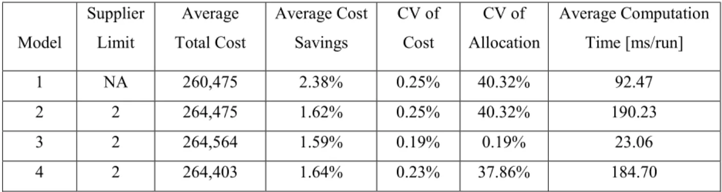
Table 13: Optimization and sensitivity analysis results of scenario 2 5.3. Scenario 3

Scenario 3 includes bids submitted from 3 suppliers. The scenario included seven items aggregated from 57 line-items. The cost matrix is shown in Table 14.

Item 1 3,753 3,553 3,708 Item 2 78,176 85,994 85,994 Item 3 119,185 116,917 121,570 Item 4 1,350 1,363 1,504 Item 5 42,121 42,453 43,930 Item 6 16,809 11,206 16,809 Item 7 16,809 8,965 16,809

(41)

41 Fixed costs were determined based on indirect coordination costs and shown in Table 15.

Fixed Costs Supplier 1 2000 Supplier 2 2000 Supplier 3 2000 Table 15: Scenario 3 fixed costs The normalized cost matrix is shown in table 16.

Item 1 0.7759 -1.1286 0.3527 Item 2 -1.1547 0.5774 0.5774 Item 3 -0.0167 -0.9916 1.0082 Item 4 -0.6508 -0.5006 1.1514 Item 5 -0.7412 -0.3962 1.1374 Item 6 0.5774 -1.1547 0.5774 Item 7 0.5774 -1.1547 0.5774

The data shows that Supplier 1’s cost is significantly lower than competitors on Item 2. Supplier 2 is dominant across most items and very dominant on items 6 and 7. An interesting note is the identical prices of items 6 and 7 for both Supplier 1 and Supplier 3. This is an example of both price matching as well as cost redistributing and may be an indication of collusion between the two suppliers.

(42)

42 Discounts applied to each supplier were sampled from a triangular distribution with parameters shown in Table 17 (all values are in %/100k OMR).

1 0 0.5% 1%

2 0 0.5% 1%

3 0 0.5% 1%

Model Supplier Limit Average Total Cost Average Cost Savings CV of Cost CV of Allocation Average Computation Time [ms/run] 1 NA 260,475 2.38% 0.25% 40.32% 92.47 2 2 264,475 1.62% 0.25% 40.32% 190.23 3 2 264,564 1.59% 0.19% 0.19% 23.06 4 2 264,403 1.64% 0.23% 37.86% 184.70

(43)

43 5.4. Scenario 4

Scenario 4 includes bids were submitted from four suppliers. The scenario included 16 items aggregated from 198 line-items. The cost matrix is shown in table 19.

Supplier 1 Supplier 2 Supplier 3 Supplier 4 Item 1 3,607 534 662 2,982 Item 2 1,407 2,450 1,684 1,268 Item 3 8,017 13,370 3,580 5,537 Item 4 4,025 7,454 2,929 4,196 Item 5 3,625 6,575 2,594 3,767 Item 6 3,625 6,575 2,594 3,767 Item 7 3,431 6,198 2,444 3,545 Item 8 2,946 5,486 2,135 3,150 Item 9 69 157 44 63 Item 10 3,030 2,094 1,600 8,994 Item 11 1,880 2,094 1,600 2,177 Item 12 2,677 2,617 1,600 3,503 Item 13 3,761 3,141 1,800 3,435 Item 14 6,805 2,513 3,700 6,721 Item 15 NA NA 4,250 NA Item 16 2,597 NA 2,597 10,219 Table 19: Scenario 4 cost matrix

Fixed costs were based on contractual fixed (preliminary) costs quoted by suppliers. They are shown in Table 20.

Fixed Costs Supplier 1 12278 Supplier 2 20416

Supplier 3 0

Supplier 4 6325 Table 20: Scenario 5 fixed costs

(44)

44 The normalized cost matrix is shown in Table 21.

Supplier 1 Supplier 2 Supplier 3 Supplier 4

Item 1 1.052 -0.895 -0.814 0.656 Item 2 -0.560 1.417 -0.035 -0.823 Item 3 0.092 1.355 -0.955 -0.493 Item 4 -0.321 1.437 -0.883 -0.233 Item 5 -0.302 1.428 -0.907 -0.219 Item 6 -0.302 1.428 -0.907 -0.219 Item 7 -0.295 1.427 -0.909 -0.224 Item 8 -0.336 1.429 -0.899 -0.194 Item 9 -0.283 1.466 -0.780 -0.403 Item 10 -0.262 -0.535 -0.680 1.477 Item 11 -0.224 0.606 -1.311 0.929 Item 12 0.100 0.023 -1.282 1.160 Item 13 0.844 0.124 -1.434 0.466 Item 14 0.863 -1.118 -0.570 0.825

In this scenario, Supplier 3 is significantly lower than other suppliers for almost all items. It also has the lowest associated fixed cost. Only items 1, 2 and 14 had lower costs from other suppliers.

Discounts applied to each supplier were sampled from a triangular distribution with parameters shown in Table 22 (all values are in %/100k OMR).

1 0 23% 46%

2 0 0 0

3 0 0 0

4 0 46% 92%

(45)

45 Model Supplier Limit Average Total Cost Average Cost Savings CV of Cost CV of Allocation Average Computation Time [ms/run] 1 NA 34,059 4.91% 0.50% 26.86% 366.35 2 2 35,813 0.00% 0.00% 0.00% 685.55 3 2 35,813 0.00% 0.00% 0.00% 44.41 4 2 35,804 0.03% 0.29% 19.90% 206.76

Table 23: Optimization and sensitivity analysis results of Scenario 4 5.5. Scenario 5

Scenario 5 bids submitted from seven suppliers for the supply and installation of various components. The scenario included 4 items aggregated from 28 line-items. The cost matrix is shown in Table 24.

Supplier 1 Supplier 2 Supplier 3 Supplier 4 Supplier 5 Supplier 6 Supplier 7

Item 1 11,612 12,818 13,750 14,189 18,071 12,805 12,677

Item 2 5,589 NA NA 5,557 6,072 6,100 6,086

Item 3 29,952 NA NA 31,928 34,382 32,884 32,947

Item 4 847 973 1,699 1,481 1,654 1,069 934

Fixed costs were determined based on indirect costs associated with coordinating with multiple suppliers and are shown in Table 25.

Fixed Costs Supplier 1 2,000 Supplier 2 2,000 Supplier 3 2,000 Supplier 4 2,000 Supplier 5 2,000 Supplier 6 2,000 Supplier 7 2,000 Table 25: Scenario 5 fixed costs

(46)

Supplier 1 Supplier 2 Supplier 3 Supplier 4 Supplier 5 Supplier 6 Supplier 7

Item 1 -0.998 -0.422 0.022 0.232 2.085 -0.429 -0.490

Item 2 -1.036 NA NA -1.151 0.679 0.778 0.731

Item 3 -1.510 NA NA -0.300 1.201 0.285 0.323

Item 4 -1.075 -0.727 1.275 0.674 1.1506 -0.463 -0.835

Supplier 1 is the lowest supplier across items 1,3 and 4. Supplier 2 is lowest on Item 3 only. The structure of the cost matrix and the dominance of Supplier 1 makes allocating for this scenario almost trivial.

1 0 2% 4% 2 0 2% 4% 3 0 2% 4% 4 0 2% 4% 5 0 2% 4% 6 0 2% 4% 7 0 2% 4%

(47)

47 The results of the optimization runs (including sensitivity analyses) are shown in Table 28.

Table 28: Optimization and sensitivity analysis results of Scenario 5

5.6. Scenario 6

Scenario 6 involves bids submitted from four suppliers. The scenario included 12 items aggregated from 81 line-items. The cost matrix is shown in Table 29.

Supplier 1 Supplier 2 Supplier 3 Supplier 4 Item 1 29,440 24,354 29,120 25,958 Item 2 1,964 2,150 2,263 2,016 Item 3 3,997 4,433 4,783 4,264 Item 4 3,914 4,156 5,083 4,979 Item 5 2,880 3,688 3,140 2,839 Item 6 29,440 30,201 31,117 27,622 Item 7 11,880 10,345 9,524 9,524 Item 8 1,610 1,380 1,702 1,511 Item 9 6,640 2,996 4,133 3,669 Item 10 1,900 790 1,184 1,054 Item 11 3,820 4,041 5,021 4,911 Item 12 1,160 1,734 1,633 1,633

(48)

48 Fixed Costs Supplier 1 2,000 Supplier 2 2,000 Supplier 3 2,000 Supplier 4 2,000

Table 30: Scenario 6 fixed costs The normalized cost matrix is shown in Table 31.

Supplier 1 Supplier 2 Supplier 3 Supplier 4

Item 1 0.899 -1.158 0.769 -0.509 Item 2 -0.996 0.384 1.221 -0.609 Item 3 -1.132 0.195 1.257 -0.320 Item 4 -1.058 -0.645 0.940 0.762 Item 5 -0.657 1.410 0.007 -0.761 Item 6 -0.105 0.408 1.026 -1.330 Item 7 1.406 0.024 -0.715 -0.715 Item 8 0.431 -1.237 1.095 -0.289 Item 9 1.434 -0.857 -0.142 -0.434 Item 10 1.408 -0.932 -0.101 -0.375 Item 11 -1.037 -0.671 0.944 0.764 Item 12 -1.474 0.752 0.361 0.361

There is a significant diversity in lowest costs in this scenario. Each supplier is lowest on at least one item.

(49)

49 Discounts applied to each supplier were sampled from a triangular distribution with parameters shown in table 32 (all values are in %/100k OMR).

1 0 2% 4%

2 0 2% 4%

3 0 2% 4%

4 0 2% 4%

(50)

50 5.7. Scenario 7

Scenario 7 involves bids submitted from three suppliers. The scenario included eight items aggregated from 163 line-items. The cost matrix is shown in Table 34.

Supplier 1 Supplier 2 Supplier 3 Item 1 15,720 13,650 24,502 Item 2 2,476 2,150 3,858 Item 3 3,945 3,525 6,148 Item 4 11,025 9,800 19,747 Item 5 7,936 6,200 12,524 Item 6 16,150 41,570 22,351 Item 7 5,152 13,705 7,948 Item 8 16,890 16,890 16,890

Fixed Costs Supplier 1 2,000 Supplier 2 2,000 Supplier 3 2,000 Table 35: Scenario 7 fixed costs

(51)

Supplier 1 Supplier 2 Supplier 3 Item 1 -0.38832 -0.7476 1.135917 Item 2 -0.38819 -0.7477 1.135892 Item 3 -0.42185 -0.71995 1.141801 Item 4 -0.46073 -0.68658 1.147315 Item 5 -0.29095 -0.82226 1.113211 Item 6 -0.79526 1.122661 -0.3274 Item 7 -0.86744 1.093764 -0.22632

In this scenario, suppliers 1 and 2 are lowest across all items. Item 8 has the same value across all suppliers and may be an indication of collusion between them.

1 0 1% 2%

2 0 1% 2%

3 0 1% 2%

The results of the optimization runs (including sensitivity analysis) are shown in Table 38.

(52)

52

6. Discussion

This project presents the application of four models with different scenarios that vary the number of suppliers and items. Over all scenarios, the process achieved cumulative estimated savings between 58k OMR and 126k OMR or 2.7% and 6.4% (depending on supplier

constraints). Scenario 7 had the highest savings across all models. This is probably due to the favorable bid distribution. The advantage, in this case, of selecting multiple suppliers over just one was significant. Scenario 5 had the lowest savings (0%). This was due to Supplier 1’s dominance, rendering the optimization process redundant.

As expected, Model 1 attained larger savings than the other more constrained models as it did not consider supplier constraints and fixed costs. It also had the computational advantage over models 2 and 4 and converged to solutions faster. These two advantages can be leveraged well in larger auctions with larger numbers of suppliers and items. Model 1’s higher savings were most pronounced in scenario 4 where certain suppliers had significant fixed costs. In practice, Model 1 is recommended as a baseline and should not be used directly to make decisions. Rather, it should be used to gain insights into suppliers’ cost structures. The model does not consider the cost of coordinating multiple suppliers (fixed costs). Disregarding the coordination hurdles of managing multiple suppliers on a project can lead to poor project performance.

Results of the sensitivity analysis highlighted low variance in total costs with coefficients of variations under 1% across all scenarios. This indicates that, in terms of total cost, the models are not significantly sensitive to variations in discount rates. However, supplier allocations had higher levels of sensitivity to the discount rates. This phenomenon was especially prevalent in Model 4 which used a genetic algorithm solver. This suggests an advantage of using

(53)

non-53 deterministic methods. They can often generate a family of “good” solutions to choose from rather than providing only one “best” solution. Model 3 does not provide this advantage due to its inherently deterministic nature.

In terms of computational performance, Model 3 achieved the fastest solve times on all scenarios. This is an interesting phenomenon since Model 3 requires solving the CRA winner determination problem multiple times. However, since the input of the problem is generally small in each iteration, the solve time is low. Model 3 also lends itself well to the structure of iterative auctions where multiple rounds are held. This is a significant advantage in practice because model 3 does not make any prior assumptions about the distribution of bids.

The savings from deploying optimization-based procurement methods go beyond the quantitative findings of this project. In practice, allowing combinatorial bidding will generally increase the competitiveness of incumbent suppliers. In parallel, they also incentivize smaller suppliers with capacity limits to bid on subsets of scenarios. These non-tangible advantages may even outweigh the short-term cost savings associated with CRAs.