HAL Id: hal-01439120
https://hal.inria.fr/hal-01439120
Submitted on 18 Jan 2017
HAL is a multi-disciplinary open access
archive for the deposit and dissemination of
sci-entific research documents, whether they are
pub-lished or not. The documents may come from
teaching and research institutions in France or
abroad, or from public or private research centers.
L’archive ouverte pluridisciplinaire HAL, est
destinée au dépôt et à la diffusion de documents
scientifiques de niveau recherche, publiés ou non,
émanant des établissements d’enseignement et de
recherche français ou étrangers, des laboratoires
publics ou privés.
T 1 mapping, AIF and Pharmacokinetic Parameter
Extraction from Dynamic Contrast Enhancement MRI
Data
Gilad Liberman, Yoram Louzoun, Olivier Colliot, Dafna Bashat
To cite this version:
Gilad Liberman, Yoram Louzoun, Olivier Colliot, Dafna Bashat. T 1 mapping, AIF and
Pharmacoki-netic Parameter Extraction from Dynamic Contrast Enhancement MRI Data. MICCAI Workshop on
Multimodal Brain Image Analysis MBIA 2011, 2011, Toronto, Canada. pp.76 - 83,
�10.1007/978-3-642-24446-9_10�. �hal-01439120�
Parameter Extraction from Dynamic Contrast
Enhancement MRI Data
Gilad Liberman1,3,4, Yoram Louzoun2, Olivier Colliot3, and Dafna Ben Bashat4
1 Gonda Multidisciplinary Brain Research Center, Bar Ilan University, Ramat Gan,
Israel,
2Department of Mathematics, Bar Ilan University, Ramat Gan, Israel, 3 Universit´e Pierre et Marie Curie-Paris 6, CNRS UMR 7225, Inserm UMR S 975,
Centre de Recherche de l’Institut Cerveau-Moelle (CRICM), Paris, France,
4 Imaging Department, Whol Institute for Advanced Imaging, Sourasky Medical
Center, Tel Aviv, Israel
Abstract. Dynamic contrast enhanced (DCE) magnetic resonance imag-ing (MRI) is a sensitive, noninvasive technique for the assessment of mi-crovascular properties of the tissue. Quantitative physiological param-eters can be obtained using pharmacokinetic (PK) models that track contrast agents as it passes through the tissue vasculature. Such analysis usually requires prior knowledge of the voxels’ T1values and of the
Arte-rial Input Function (AIF). Therefore, relaxometry T1measurements are
usually performed prior to contrast-agent injection and the AIF is man-ually or automatically extracted from the dynamic data. In this study, a method for a fully automatic analysis of DCE data for joint PK param-eters, T1 mapping and AIF extraction is proposed. Results are shown
on simulated data compared to other methods and on data acquired from healthy subjects and patients with Glioblastoma who received anti-angiogenic therapy. The proposed method renders DCE analysis to be robust and easily applicable.
1
Introduction
Dynamic contrast enhancement (DCE) Magnetic resonance imaging (MRI) is a noninvasive method that provides vasculature information about the tissue. This method was shown to be sensitive and often used as indicator to monitor response to anti-angiogenic drugs in several organs including the brain [1]. In DCE, repeated T1 weighted images are acquired with high temporal resolution,
during the administration of a contrast agent resulting in a signal intensity time curve Sv(t), at each voxel. This dynamic information shows the rate at which
tissue enhances, and afterwards, the rate at which contrast agent washes out. The time curve can be converted into a contrast agent concentration time curve C(t) and using a pharmacokinetic (PK) model, several physiological parameters can be extracted, such as vessels permeability, the volumes of the vessel and the extra-vascular extra-cellular space.
2
In order to obtain the concentration time curve, a prior knowledge on the T1
values within each voxel is needed. Therefore, a T1 relaxometry experiment is
performed prior to the DCE experiment. Inversion-recovery (IR) and saturation-recovery (SR) are the principal methods for T1 measurements, yet their long
acquisition times make them inapplicable for clinical use. Several alternative methods have been proposed for rapid and accurate measurement of the longi-tudinal relaxation time T1. A commonly used method is the variable nutation
angle method, that use a collection of spoiled gradient echo (SPGR) images over a range of flip angles. Although this method allows quick T1 determination, it
requires additional scanning and often suffers from B1inhomogeneity, and errors
result from inaccurate flip angle.
Following this stage, the C(t) is fitted to a PK model. Several PK mod-els have been proposed including the general kinetic model, Patlak model and Tofts model [13]. This study used the extended Tofts-Kety model [9]. Most of the models require an auxiliary Arterial Input Function (AIF), which is C(t) in the artery feeding the examined voxels. The AIF is artery, patient and scan dependent. Several studies suggest using common population average AIF such as the one provided by [7]. The AIF can also be approximated by averaging several C(t)s from voxels inside major arteries, which can be located manually or automatically. These approaches require that the scan time-resolution will be high enough for accurate AIF determination. Fit-based methods for extract-ing the AIF from C(t)s of multiple regions have been recently reported [5, 12], where extraction of the AIF and PK parameters from the C(t)s are performed alternately using an expectation-maximization like algorithm, which is prone to local-minima problems. Yang [12] has noted the advantage of calculating the AIF at a higher time resolution than the scanning one, while Fluckiger [5] addressed the same problem by fitting the extracted AIF into a parametric formulation. We suggest a direct search over a parametric formulation of the AIF, thus less dependent on start point and local minimas.
While previously reported methods fitted the model to the C(t), the algo-rithm proposed in this study fits the model and a T1 value to the signal ratio
to baseline curve. This enables us to extract the T1 values from the DCE data
itself, thus not requiring additional scan for T1mapping. Furthermore, using the
signal ratio to baseline curve as a standard of reference enables a fair comparison between different algorithms, whereas comparison based on the C(t) curves adds additional varables and necessitate additional calculation which depends on the analysis software / algorithm, and complicates comparison. The incorporation of the T1value into the fitting scheme renders the problem non-linear.
Several algorithms have been suggested for fitting of the C(t) in order to extract PK parameters given the AIF. Murase [2] has formulated the differ-ential equations of the extended Tofts-Kety model into simple matrix multi-plication, resulting in a very efficient extraction of parameters. However this method implicitly assumes that the AIF can be approximated by its discrete low time-resolution form, and indeed was found in our study to be inaccurate, especially in sensitive areas such as those with low Signal-to-Noise Ratio (SNR),
where the resulting inaccuracies are more pronounced. We propose a simple search over the non-linear term in the convolution formulation of the model. This enables the computation to be made in arbitrary time-resolution. We com-pare and evaluate our algorithm with Murase’s as well as common non-linear curve-fitting techniques, including Simplex Simulated Annealing and Fletcher-Levenberg-Marquardt algorithm [4, 3].
The following sections are organized as follows. Background and the proposed approach are presented in §2. The experiments and their results are discussed in §3 and the conclusions are given in §4.
2
Methods
2.1 Calculating the signal ratio to baseline curve
DCE MRI is usually acquired using a spoiled gradient echo (SPGR) sequence. The signal follows this equation [8]
S = M0
(1 − E1) sin(α)
1 − E1cos(α)
. (1)
where α is the flip angle, E1= exp(−T R/T1) and M0includes the proton density,
T2and T2∗contributions and any fixed factor resulting from scanner settings. TR
and FA are the repetition time and flip angle which are scan parameters and are fixed during the scan. The tissue’s T1 value is changing during the experiment
as a function of the contrast agent concentration C(t):
∆R1(t) = R1(t) − R10= r1· C(t). (2)
where R10 = 1/T1 is the relaxation rate at baseline (without contrast agent),
R1(t) is the relaxation at time t and r1is the relaxivity coefficient of the contrast
agent. Ξ = S(t) S0 =(1 − E10)(1 − E1(t) cos(α)) (1 − E1(t))(1 − E10cos(α)) . (3)
Where E1(t) = exp(−T R · R1(t)). The baseline value S0 can be computed by
averaging the signal before contrast agent administration. The M0term includes
a multiplicative exp(−T E/T∗
2) term. Although T2∗ changes in the presence of
contrast agent, its effect on the signal is negligible due to the low TE values used in SPGR sequences.
2.2 Extraction of the PK parameters and T1 values
Given T1, C(t) can be extracted from the signal ratio to baseline Ξ(t) using
equation (3). C(t) can be modeled using the Extended Tofts-Kety model [9] by d(Ct− vpAIFt)
4
where AIF is the Arterial Input Function, the concentration of contrast agent in the feeding artery. The AIF is assumed to be the same for the whole analyzed volume of interest (VOI). ktransand k
epare the transfer rates between the blood
plasma to the extra-vascular extra-cellular and back, respectively. veand vp are
the extra-vascular extra-cellular and the plasma relative volumes, respectively. The solution of the differential equation for C(t) with initial conditions AIF0=
C0= 0 was given by [9]
C(t) = ktrans(AIF (t) ∗ exp(−kept)) + vpAIF (t). (5)
Where ∗ means convolution. The important pharmacokinetic parameter ktrans
is equal to vekep. Following [2], integrating (4) leads to
C(t) = (ktrans+ kepvp) Z t 0 AIF (u)du − kep Z t 0 C(u)du + vpAIF (t). (6)
Discretizing, denote by −−−−→SAIF and −→SC the cumulative sums of the AIF and the tissue contrast agent concentration curve, respectively, in the samples time points. The equation system resulting from (6) can thus be expressed in matrix form as −→
C = (−−−−→SAIF −−→SC −−→AIF )−→XT. (7)
− →
X = (ktrans+ kepvp kep vp)
where vectors are columns and ·T means transpose. Given the AIF, X can
be extracted by minimizing the least squares error and the PK parameters ktrans, k
ep, ve, vpare approximated. Murase’s method implicitly assumes that the
AIF and the Cts can be accurately approximated by the piecewise-linear curve
induced by the data vectors. This might fail when the acquisition time-resolution is not high enough. Indeed, Murase’s method was found to be inaccurate in our simulations and data for low SNR values. Therefore an alternative method, based on equation (5), is proposed in this study. Given the AIF and kep, the equation
system can be formulated as − → C = (−−−−−−−−−−−−→AIF ∗ exp(kepu) −−→ AIF )−→YT. (8) − → Y = (ktrans vp)
and solved similarly. The solution was compared to the solution given while fixing either ktrans or v
p for their minimal and maximal values, and the one
with minimal error was selected. Finding the correct kep is found by exhaustive
search, i.e. repeating the process for several values of kep (21 values, spaced
non-uniformly in [0,max kmin vtranse =
2.2
0.15 = 14.667]min−1).
We suggest finding T1by fitting to the signal ratio to baseline curve Ξ using
exhaustive search in biological range (22 values spaced uniformly in [300, 4000]ms). For each T1 value, Ct is calculated from Ξ using eq. (3) and the PK
(8) (given final AIF). Using the PK parameters and T1, we simulate the signal
ratio to baseline curve ˆΞ and compare it to Ξ using the Euclidean norm. Added penalty on improbable T1 values can be used at this level, corresponding, in
a Bayesian interpretation, to prior on the expected T1 in the voxel, which can
result from relaxometry or segmentation. The simulation is done using equation (5) and requires convolution. Both the AIF and exp(kept) can be calculated for
arbitrary time points, and this convolution is calculated numerically in higher time resolution to increase accuracy.
We compare the results obtained using the proposed method with Murase’s method, a conventional fitting method [3] and a fast simulated annealing variant [4]. For estimating the inaccuracies resulting from fit-based T1 approximation,
results are compared based on simulated data with the parameters estimated by the mentioned methods with given true T1 values.
2.3 AIF extraction
Parker [7] has suggested to model the AIF using two Gaussians and a sigmoid which correspond to the main and second cycle contrast agent boluses and the washout: AIF = 2 X i=1 AiN (τi, σi) + α exp(−βt) (1 + exp(−s(t − τ0))) . (9)
Where N is the normal distribution. Mean values for the model parameters were also given. (9) can be modified to yield a version more fitted for function search by using relative values for the amplitudes (A2, α relative to A1) and
times (τ2, τ0 relative to τ1). We denote by AIF f () the AIF model given by the
modified version of (9).
The proposed cost function is the maximum over the sum square error for the given signal ratio to baseline curve, normalized by its maximum minus one, i.e. its maximal relative enhancement value.
arg min θ max i∈Clusters k ˆΞiAIF f (θ)− Ξik2 maxjΞi(j) − 1 . (10)
On real data, the curves used are the result of a cluster analysis over all of the brain’s voxels (healthy subjects) or a large VOI around the lesion (patients). The VOI is masked by the following criteria - Minimal enhancement of 2%, a signal over a specific threshold value (experimental defined) and probability of being a gray or white matter tissue more than 30% (as defined using SPM’s segmenta-tion module [11]). The cluster analysis used is Expectasegmenta-tion-Maximizasegmenta-tion (EM) over Mixture of Gaussians (MoG) model [6] with 100 clusters. The clustering is calculated over the voxels’ signal curves (rather than the signal ratio to baseline curve). The bolus starting point is approximated in a competitive manner by clustering the medians of the signals of all the brain volume at each time point into 3 clusters and selecting the first value which is classified into a cluster differ-ent than that of the first time point. Voxels for which the maximal enhancemdiffer-ent
6
occurs more than one acquisition before the approximated bolus starting point are masked out. The search was done by running SIMPSA [4] twice. The first run uses the parameters given by Parker [7] as a starting point and works on a reduced set of data for acceleration. In a second step, more clusters are used, and the result of the first run is the starting point. Up to 5 clusters are automatically chosen for the first SIMPSA run by selecting the clusters with the highest max-imal signal to baseline ratio, while assuring that at least 2 clusters with visible contribution of the plasma to C(t) are selected. For the second run, 40 clusters are randomly chosen. Clusters with noisy curve are discarded.
3
Experiments and results
Simulated data. To test the extraction of the PK parameters, 500 signal ratio to baseline curves were simulated using the AIF given at [7], with T1 and PK
parameters selected randomly in biological ranges (T1in [300, 4000] ms, ktransin
[0, 2.2] min−1, v
e in [0.15, 1], vp in [0, 0.3]). Mean Absolute Relative Difference
(ARD) was used as the statistical criteria.
Results of the simulated data, obtained using the proposed method compared to SIMPSA, FLM and Murase’s method, are reported in Table 1. Note that the proposed method yield the smaller ARD values for all parameters with and without prior knowledge of T1 values, compared to the other methods.
For AIF extraction tests, 100 runs were done with the AIF model of eq. (9) on randomly selected parameters around the ones given in [7] (between half and double the reported value, except for τ1, between 0.8 to 3 times the reported
value). Additionally, a small amount of noise on the AIF model parameters was added to each simulated voxel (Multiplicative factor of N (1, 0.05)) to simulate the changes in AIF between feeding artery in the VOI. Finally, an additive Gaussian noise (σ = 0.08) was added to the simulated signal ratio time curve to simulate noise in acquisition. This noise amplitude was extracted by the std. of the signal before contrast agent administration for a representative patient. We used r1= 1. This value gave maximal signal ratio curve values similar to ones
observed in real data (around 6).
Results are reported in Table 2. The proposed method using SIMPSA yielded the smallest ARD values for the PK parameters, excluding kep.
Method ktransve vp T1 ktransve vp
SIMPSA 2.66 0.82 1.66 0.42 1.54 0.56 0.72
FLM 2.73 0.71 0.70 0.52 1.57 0.91 0.74
Murase 0.94 1.08 1.09 0.45 0.30 0.50 0.46
Proposed method 0.67 0.54 0.57 0.42 0.22 0.12 0.16
Table 1.Comparison of mean ARD values for the PK parameters. The last 3 columns show results when T1 was assumed to be known. For Murase’s method, the T1 value
PK Method AIF Method ktransv
e vp T1 kep
Murase SIMPSA 0.93 1.50 0.68 0.52 0.50
Murase SIMPSA, full data 1.02 1.91 0.69 0.59 0.59 Murase SIMPSA, 2 steps 1.00 1.80 0.70 0.58 0.59 Proposed method SIMPSA 0.75 0.83 0.54 0.55 0.52 Proposed method SIMPSA, full data 0.88 1.11 0.57 0.59 0.61 Proposed method SIMPSA, 2 steps 0.97 1.08 0.59 0.60 0.67
Table 2.Comparison of mean ARD values for the PK parameters, after AIF estimation using only clusters with strong enhancement, using all data or in two steps.
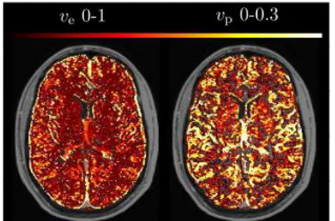
MRI data. The proposed algorithm was tested on real MRI data obtained from five healthy controls and five longitudinal studies of two patients with progressive recurrent glioblastoma along the administration of an anti-angiogenic therapy (Bevacizumab) combined with Irinotecan. The signal ratio to baseline curves were fitted accurately for all studies. For the control group, the different vascular regions are clearly visible (see Fig. 1 top). A representative result for a longitudinal study of a patient with Glioblastoma is shown in Fig. 1 left. As expected, after two weeks of anti-angiogenic therapy, a reduction of ktrans and
vp is visible in the tumor area.
ktrans0-2.2 v p0-0.3
Time 0
Week 2
ve0-1 vp0-0.3
Fig. 1.Left: ktransand v
p(columns) maps
for a longitudinal study of a patient with GBM. Weeks 0, 2 (rows) of anti-angiogenic treatment. Top: ve and vp maps for a
healthy subject, showing vascular regions.
4
Conclusion
This work proposes a method for PK parameters extraction by curve fitting to the DCE data. The choice of fitting to the actual DCE data rather than concentration time curves approximated using pre-computed T1 values renders
the method more applicable to acquired data and independent of relaxometry calculation. The automatic identification of the AIF renders the method fully au-tomatic. The pseudo-sampling during calculation enables the system to maintain accuracy while retaining high efficacy through matrix operations. The method
8
has been applied to both simulated and real data resulting in good results. Future work will incorporate optimizing global parameters such as the flip angle.
Acknowledgments and Funding. This work was supported by the James S. McDonnell Foundation number 220020176. We are grateful to the patients and their families, who so willingly participated in this study and to Vicki Meiers for editorial assistance.
References
1. O’Connor, J.P.B., Jackson, A., Parker, G.J.M., Jayson, G.C.: DCE-MRI biomarkers in the clinical evaluation of antiangiogenic and vascular disrupting agents. Brit. J. Can. 96, 189–195(2007)
2. Murase, K.: Efficient method for calculating kinetic parameters using T1-weighted dynamic contrast-enhanced magnetic resonance imaging. Mag. Res. Med. 51, 858– 862 (2004)
3. Fletcher, R.: A modified Marquardt subroutine for nonlinear least squares. Atom. Res. Est. AERE-R6799 (1971)
4. Cardoso, M.F., Salcedo, R., Feyo de Azevedo, S.: The simplex-simulated annealing approach to continuous non-linear optimization. Comp. Chem. Eng. 20, 1065-1080 (1996)
5. Fluckiger, J.U., Schabel, M.C., DiBella, E.V.R.: Model-based blind estimation of kinetic parameters in dynamic contrast enhanced (DCE)-MRI. Mag. Res. Med. 62, 1477–1486 (2009)
6. Bouman, C. A., Shapiro, M., Cook, G. W., Atkins, C. B., Cheng, H.: Cluster: An unsupervised algorithm for modeling gaussian mixtures, https://engineering. purdue.edu/~bouman/
7. Parker, G. J., Roberts, C., Macdonald, A., Buonaccorsi, G. A., Cheung, S., Buckley, D. L., Jackson, A., Watson, Y., Davies, K., Jayson, G. C.: Experimentally-derived functional form for a population-averaged high-temporal-resolution arterial input function for dynamic contrast-enhanced MRI. Mag. Res. Med. 56, 993–1000 (2006) 8. Deoni, S. C., Rutt, B. K., Peters, T. M.: Rapid combined T1 and T2 mapping using gradient recalled acquisition in the steady state. Mag. Res. Med. 49, 515–526 (2003) 9. Tofts, P. S., Kermode, A. G.: Measurement of the blood-brain barrier permeability and leakage space using dynamic MR imaging. 1. Fundamental concepts. Mag. Res. Med. 17, 357–367 (1991)
10. Tofts, P. S., Brix, G., Buckley, D. L., Evelhoch, J. L., Henderson, E., Knopp, M. V., Larsson, H. B., Lee, T.-Y., Mayr, N. A., Parker, G. J., Port, R. E., Taylor, J., Weisskoff, R. M.: Estimating kinetic parameters from dynamic contrast-enhanced t1-weighted MRI of a diffusable tracer: Standardized quantities and symbols. J. Mag. Res. Imag. 10, 223–232 (1999)
11. Ashburner, J., Friston, K.J.: Unied segmentation. NeuroImage 26, 839–851 (2005) 12. Yang, C., Karczmar, G. S., Medved, M., Stadler, W. M.: Multiple reference tissue method for contrast agent arterial input function estimation. Mag. Res. Med. 58, 1266–1275 (2007)
13. Srikanchana, R., Thomasson, D., Choyke, P., Dwyer, A.: A Comparison of Pharma-cokinetic Models of Dynamic Contrast Enhanced MRI. In: 17th IEEE Symposium on Computer-Based Medical Systems, pp. 361. IEEE Computer Society, Los Alami-tos (2004)